http://www.sciencepublishinggroup.com/j/ijbse doi: 10.11648/j.ijbse.20190702.12
ISSN: 2376-7227 (Print); ISSN: 2376-7235 (Online)
Using Data Mining Algorithms for Thalassemia Risk
Prediction
Ngozi Chidozie Egejuru
1, Sekoni Olayinka Olusanya
2, Adanze Onyenonachi Asinobi
3,
Omotayo Joseph Adeyemi
2, Victor Oluwatimilehin Adebayo
4, Peter Adebayo Idowu
41Department of Computer Science, Hallmark University, Ijebu-Itele, Nigeria 2
Department of Computer Science, Tai Solarin University of Education, Ijebu Ode, Nigeria 3
Department of Pediatrics, College of Medicine, University of Ibadan, Ibadan, Nigeria
4Department of Computer Science and Engineering, Obafemi Awolowo University, Ile-Ife, Nigeria
Email address:
To cite this article:
Ngozi Chidozie Egejuru, Sekoni Olayinka Olusanya, Adanze Onyenonachi Asinobi, Omotayo Joseph Adeyemi, Victor Oluwatimilehin Adebayo, Peter Adebayo Idowu. Using Data Mining Algorithms for Thalassemia Risk Prediction. International Journal of Biomedical Science and Engineering. Vol. 7, No. 2, 2019, pp. 33-44. doi: 10.11648/j.ijbse.20190702.12
Received: August 7, 2019; Accepted: August 23, 2019; Published: September 6, 2019
Abstract:
This study predict the risk of thalassemia in all age groups based on identified risk of thalassemia. Knowledge about the risk factors for thalassemia was identified using structural interview with experienced medical personnel and questionnaire which was used to collect empirical medical database on the parameters. Supervised machine learning algorithms was used to formulate the predictive model for risk of thalassemia using the parameters and data identified and collected. The predictive model for the risk of thalassemia was simulated using the Waikato Environment for Knowledge Analysis (WEKA). The simulated model was validated using the historical data collected from the hospitals explaining the parameters and the risk of Thalassemia. The results of the study showed that following the collection of data from 51 patients, the parameters identified included demographic variables like gender, age, marital status, ethnicity and social class while the clinical variables included family history, spleen enlargement, diabetes, urine colour changes and parent carriers while the distribution of the risk was 43% no cases, 10% low cases, 16% moderate cases and 31% high cases. The study concluded that using the multi-layer perceptron for the prediction of Thalassemia will improve the decision making process within the healthcare service concerning Thalassemia.Keywords:
Thallasemia, Anaemia, Predictive Model, Naïve Bayes, Classifier, Multilayer Perceptron1. Introduction
Thalassemia is an inherited blood disorder in which the body makes an abnormal form of hemoglobin. Hemoglobin is the protein molecule in red blood cells that carries oxygen. The disorder results in excessive destruction of red blood cells, which leads to anemia [1]. The World Health Organization (WHO) defines Aneamia as a hemoglobin value below 13 g/dl in men over 15 years of age, below 12g/dl in non-pregnant women over 15 years, and below 11g/dl in pregnant women [2]. It is a condition in which the number of red blood cells or their oxygen carrying capacity is insufficient to meet physiologic needs and this varies for age, sex, altitude and pregnancy status [3]. Aneamia is a global
public health problem affecting both developed and developing countries.
consequences of Aneamia in children are inimical as it affects their cognitive performance, behaviour and physical growth. Children who suffer from Aneamia have delayed psychomotor development and impaired performance of tests; in addition, they experience impaired coordination of language and motor skills, equivalent to a 5 to 10 points deficit in intelligent quotient (IQ) [3]. In Southern Asia, the prevalence of Aneamia in pregnancy is about 75% in contrast to what obtains in North America and Europe with about 17% prevalence. Furthermore, 5% of pregnant women suffer from severe Aneamia in the worst affected parts of the world [7].
Data mining concept is sorting the data to identify patterns and find relationships between these data. It is techniques are appropriate for simple or structured datasets such as relational databases, transactional databases. Different approaches of data mining proposed to improve the challenges of storing and processing all types of data [8, 9]. Data mining has three basic mechanisms Clustering (Classification), Decision Rules and Analysis. Classification analyzes a set of data and produces a set of decision rules, which used to classify the data sets. In the artificial intelligence, machine learning or database systems data mining process is starting by extract the information from dataset then convert it to meaning full structure. This means that it determines patterns in datasets and embracing methods. There are many classes in data mining where the most common one is classification, which is used to predict set of relationship between data. In healthcare, it is significant to invest the development in computer technology to enhance processing the medical data such as data mining classification algorithms and tools.
There are growing researches interest in using data mining in the medical domain. Developing in this new approach, called medical data mining, concerned with developing systems that determine and predict knowledge from data generating from medical environments. The data mining in the medical domain specifically the hospital database, including the data, which is huge in amounts, complex in contents, with heterogeneous types, hierarchical and varying in quality. Among last years, the information on laboratories keeps on enhancing and developing. The specific patterns of information can predicated through using data mining methodologies to enhance conducting researches and evaluation of reports. The data mining classification depends on similarities existing in the data.
Existing techniques do not apply knowledge discovery rather they rely on human knowledge which may be skewed or limited. Therefore, there is a need to apply knowledge discovery techniques using data mining algorithms for the development of a classification model for the risk of thalassemia in Nigerians. Therefore, this study attempts to apply data mining algorithms in the development of a predictive model which can be used to predict the risk of thalassemia in Nigerians of all age groups based on medical information important for identifying the risk of thalassemia.
2. Related Works
In 2011, Chuang et al. worked on DNA repair genes in order to better predict oral cancer by choosing a single nucleotide polymorphisms (SNPs) dataset [10]. The chosen dataset had certain samples of oral cancer’s patients. In this research, by using the support vector machines all prediction experiments were performed. On the basis of experimental result, it has been found that the performance of holdout cross validation was better than the performance of 10-fold cross validation. Apart from this, it has been also found that the accuracy of classification was 64.2%.
In 2006, Hu et al. used different types of classification methods such as decision trees, SVMs, Bagging, Boosting and Random Forest for analyzing microarray data [11]. In the research, experimental comparisons of LibSVMs, C4.5, Bagging C4.5, AdaBoosting C4.5, and Random Forest on seven micro-array cancer data sets were conducted using 10-fold cross validation approach on the data sets obtained from Kent Ridge Bio Medical Dataset repository. On the basis of the experimental results, it has been found that Random Forest classification method performs better than all the other used classification methods.
Huang et al constructed a hybrid SVM-based diagnosis model in order to find out the important risk factor for breast cancer because in Taiwan, women especially young women suffered from breast cancer [12]. In order to construct the diagnosis model, several types of DNA viruses in this research are studied. These DNA viruses are HSV-1 (herpes simplex virus type-1), EBV (Epstein-Barr virus), CMV (cytomegalovirus), HPV (human papillomavirus), and HHV-8 (human hepesvirus-HHV-8). On the basis of experimental results, either {HSV-1, HHV-8} or {HSV-1, HHV-8, CMV}can achieved the identical high accuracy. The main aim of the study was to obtain the bioinformatics about the breast cancer and DNA viruses. Apart from SVM-based model, another type of diagnosis model called LDA (Linear discriminate analysis) was also constructed in this research.
In 2009 Curiac et al. analyzed the psychiatric patient data using the Bayesian Networks (BN) in order to identify the most significant factors of psychiatric diseases and their correlations by performing experiment on real data obtained from Lugoj Municipal Hospital [13]. In this research, it has been found that BBN plays a very important role in medical decision making process in order to predicate the probability of a psychiatric patient on the basis detected symptoms.
Amin and Habib [14], have compared between naïve Bayes, J48 classifier and neural network classification algorithms using WEKA and working on hematological data to specify what the best and appropriate algorithm. The proposed model can predict hematological data and the results showed that the best algorithm is J48 classifier with high accuracy and naïve Bayes is the lowest average in average errors.
logic using three (3) clinical variables while the rules for the inference engine were elicited from expert pediatrician. The fuzzy logic-based model was not validated using live clinical datasets. Moreover, relevant variables for SCD survival could have been easily identified using feature selection methods from a larger collection of variables monitored for pediatric SCD survival.
3. Methods
This section highlights the methodology design applied in the development of the predictive model for the risk of Thalassemia in a well-detailed manner. The methodology consists of a sequence of methods/techniques which started with the identification of the variables predictive of risk of Thalassemia alongside the data collection method used in gathering the required data needed for model development. The historical data collected contained records of patients
consisting of their respective values for each identified variables as inputs alongside the target variable (risk of Thalassemia) as the output variable.
3.1. Data Identification and Collection
Following the review of related works of literature in the body of knowledge of risk of Thalassemia and the variables related to determine risk of Thalassemia, a number of variables were identified. The identified variables for determining risk of Thalassemia were validated by a medical physician interviewed with more than 10 years’ experience in medicine before the data was collected from the hospital located in the south-western part of Nigeria. For the purpose of this study, data was collected from 49 patients undergoing treatment at a hospital located in the south-western part of Nigeria from hospital case files. A description of the attributes contained in the dataset is shown in Table 1.
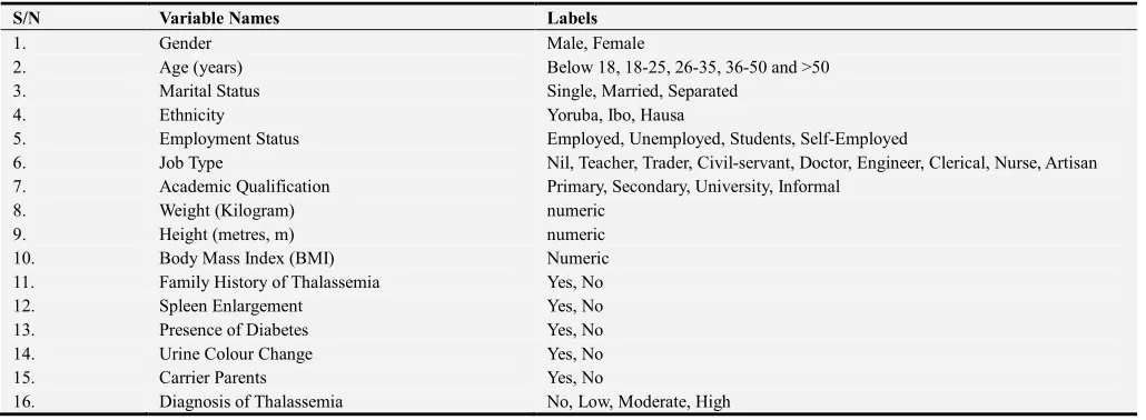
Table 1. Identified variables for determining thalassemia.
S/N Variable Names Labels
1. Gender Male, Female
2. Age (years) Below 18, 18-25, 26-35, 36-50 and >50
3. Marital Status Single, Married, Separated
4. Ethnicity Yoruba, Ibo, Hausa
5. Employment Status Employed, Unemployed, Students, Self-Employed
6. Job Type Nil, Teacher, Trader, Civil-servant, Doctor, Engineer, Clerical, Nurse, Artisan
7. Academic Qualification Primary, Secondary, University, Informal
8. Weight (Kilogram) numeric
9. Height (metres, m) numeric
10. Body Mass Index (BMI) Numeric
11. Family History of Thalassemia Yes, No
12. Spleen Enlargement Yes, No
13. Presence of Diabetes Yes, No
14. Urine Colour Change Yes, No
15. Carrier Parents Yes, No
16. Diagnosis of Thalassemia No, Low, Moderate, High
3.2. Data Preprocessing
Following the collection of data from the 49 patients alongside the attributes (16 risk factors) alongside the diagnosis of Thalassemia, the data collected was checked for the presence of error in data entry including misspellings and missing data. Subsequently, the data was transformed into the attribute file format (arff) for the purpose of the development of the predictive model for infertility risk using the simulation environment.
3.3. Formulation of Predictive Model for Classification of Risk of Thalassemia
For any supervised machine learning algorithm proposed for the formulation of a predictive model, a mapping function can be used to easily express the general expression for the formulation of the predictive model for the classification of risk of Thalassemia-this is as a result that most machine learning algorithms are black-box models which use evaluators and not power series/polynomial equations. The
historical dataset S which consists of the records of patients containing fields representing the set of classification factors (i number of input variables for j patients), alongside the respective target variable (risk of Thalassemia) represented by the variable - the risk of Thalassemia for the jth
individual in the j records of data collected from the hospital selected for the study. Equation 1 shows the mapping function that describes the relationship between the classification factors and the target class-classification of risk of Thalassemia.
: → (1)
: =
used to represent the predictive model for patient performance maps the variables of each individual to their respective risk of Thalassemia according to equation 2.
= !
" #ℎ
(2)
The developed predictive model for the risk of Thalassemia was used to propose a set of rules that can be used to determine the risk of Thalassemia directly just by observing the value of the variables identified by the model and the succession of events. In the following section, the machine learning algorithms used in formulating the predictive model for the risk of Thalassemia are presented.
3.3.1. Naïve Bayes’ Classifier for Thalassemia Risk Prediction
Naive Bayes’ Classifier is a probabilistic model based on Bayes’ theorem. It is defined as a statistical classifier. It is one of the frequently used methods for supervised learning. It provides an efficient way of handling any number of attributes or classes which is purely based on probabilistic theory. Bayesian classification provides practical learning algorithms and prior knowledge on observed data.
Let be a dataset sample containing records (or instances) of i number of risks factors (attributes/features) alongside their respective diagnosis of Thalassemia, C (target class) collected for j number of records/patients and "% =
{" = , " = , " = ! , "&= " #ℎ} be a hypothesis that belongs to class C. For the classification of the risk of thalassemia given the values of the risk factor of the jth record, Naïve Bayes’ classification required the determination of the following:
a)' "%| -Posteriori probability: is the probability that the hypothesis, "% holds given the observed data sample for 1 ≤ + ≤ 4.
b)' "% - Prior probability: is the initial probability of the target class 1 ≤ + ≤ 4;
c)' is the probability that the sample data is observed for each risk factor (or attribute), i; and d)' | |"% is the probability of observing the sample’s
attribute, given that the hypothesis holds in the training data .
Therefore, the posteriori probability of an hypothesis "% is defined according to Bayes’ theorem as follows:
' "%| = ∏ ./012|345. 01
6 178
. 34 + = 1,2,3,4 (3)
Hence, the risk of Thalassemia for a record is thus:
; <. ='/" > 5, '/" > 5, '/" > 5,
'/"&> 5 ? (4)
3.3.2. Multilayer Perceptron for Thalassemia Risk Prediction
An artificial neural network (ANN) is an interconnected
group of nodes, akin to the vast network of neurons in a human brain. In machine learning and cognitive science, ANNs are a family of statistical learning models inspired by biological neural networks and are used to estimate or approximate functions that depend on a large number of inputs and are generally unknown. ANNs are generally presented as systems of interconnected neurons which send messages to each other such that each connection have numeric weights that can be tuned based on experience, making neural nets adaptive to inputs and capable of learning.
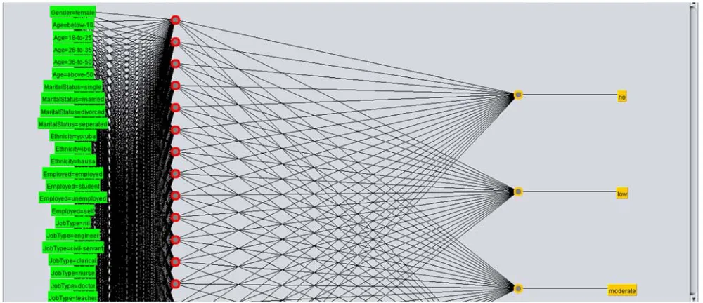
The word network refers to the inter-connections between the neurons in the different layers of each system. The first layer has input neurons (CML survival indicators) which send data via synapses to the middle layer of neurons, and then via more synapses to the third layer of output neurons (see Figure 1). The synapses store parameters called weights that manipulate the data stored in the calculations. An ANN is typically defined by three (3) types of parameters, namely:
i. Interconnection pattern between the different layers of neurons;
ii.Learning process for updating the weights of the interconnections; and
iii.Activation function that converts a neuron’s weighted input to its output activation.
Multi-layer networks use a variety of learning techniques, the most popular been back-propagation. Back-propagation, an abbreviation for backward propagation of errors, is a common method of training artificial neural networks used in conjunction with an optimization method such as gradient descent. The method calculates the gradient of a loss function with respect to all the weights in the network. The gradient is fed to the optimization method which in turn uses it to update the weights, in an attempt to minimize the loss function. It is a generalization of the delta rule to multi-layered feed-forward networks, made possible by using the chain rule to iteratively compute gradients for each layer. Back-propagation requires that the activation function used by the artificial neurons be differentiable.
The back-propagation learning algorithm can be divided into two phases: propagation and weight update.
a)Phase 1-Propagation: each propagation involves the following steps:
i. Forward propagation of training pattern’s input through the neural network in order to generate the propagation’s output activations; and
ii.Backward propagation of the propagation’s output activations through the neural network using the training pattern target in order to generate deltas of all output and hidden neurons.
b)Phase 2-Weight update: for each weight-synapse, hence the following:
i. Multiply its output delta and input activation to get the gradient of the weight; and
Figure 1. Multi-layer perceptron architecture for risk of Thalassemia.
In this study, the input neurons were represented by each Thalassemia risk indicator variables determined by Xi = {X1,
X2, X3 ….Xi} where i is the number of variables (input
neurons). The effect of the synaptic weights, Wi on each
input neuron at layer j is represented by the expression:
@ = < A < A ⋯ … < A D (5)
Equation (5) is sent to the activation function (sigmoid/logistic function) was applied in order to limit the output to a threshold [-1, +1], thus:
E = @ = F GHI2 (6)
The measure of discrepancy between the expected output (p) and the actual output (y) was made using the squared error measure (E):
J = K L M (7) Recall however, that the output (p) of a neuron depends on the weighted sum of all its inputs as indicated in equation (5); implying that the error (E) also depends on the incoming weights of the neuron which needs to be changed in the network to enable learning. The back-propagation algorithm was used to find the set of weights that minimizes the error. In this study, the gradient descent algorithm was applied in order to minimize the error and hence find the optimal weights that satisfy the problem. Since back-propagation uses the gradient descent method, there was a need to calculate the derivative of the squared error function with respect to the weights of the network. Hence, the squared error function is now redefined as (the ½ is required to cancel the exponent of 2 when differentiating):
J = K L M (8)
For each neuron, j its output Oj is defined as:
N = / ! 5 = /∑P <
%Q 5 (9)
The input ! to a neuron is the weighted sum of outputs
Nof the previous neurons. The number of input neurons is n and the variable denotes the weight between neurons I and j. The activation function is in general non-linear and differentiable, thus, the derivative of the equation (6) is:
RS
RT= 1 L (10)
The partial derivative of the error (E) with respect to a weight was done using the chain rule twice as follows:
RU RV12
RU RW2
RW2 RPGX2
RPGX2
RV12 (11)
The last term on the left hand side can be calculated from equation (3.15), thus:
RPGX2 RV12
R
RV12/∑ < P
%Q 5 < (12)
The derivative of the output of neuron j with respect to its input is the partial derivative of the activation function (logistic function) shown in equation (10):
RW2 RPGX2
R
RPGX2 / ! 5 / ! 5 Y1 L / ! 5Z (13)
The first term is evaluated by differentiating the error function in equation (13) with respect to y, so if y is in the outer layer such that y = N, then:
RU RW2
RU R[
R
R[ K L M M L K (14)
RU
RW2 ∑ \
RU RPGX]
RPGX] RW2^
_`a ∑ Y_`a RWRU] RPGXRW]] _Z (15)
Thus, the derivative with respect to Ncan be calculated if all the derivatives with respect to the outputs Nof the next layer-the one closer to the output neuron-are known. By
putting them all together:
RU
RV12 b < (16)
With:
b cNcJ c !cN d/N L K 5 / ! 5 Y1 L / ! 5Z e f!Kf! f ,
g b _ / ! 5 Y1 L / ! 5Z e f
_`a
Therefore, in order to update the weight using gradient descent, one must choose a learning rate, h. The change in weight, which was added to the old weight, is equal to the product of the learning rate and the gradient, multiplied by-1:
∆ LhRVRU12 (17)
Equation (17) was used by the back-propagation algorithm to adjust the value of the synaptic weights attached to the inputs at each neuron in equation (5) with respect to the inner layer of the multi-layer perceptron classifier.
3.4. Model Simulation Process and Environment
Following the identification of the supervised machine learning algorithms that was needed for the formulation of the predictive model for the classification of risk of Thalassemia, the simulation of the predictive model was performed using the data collected which consisted of patients records containing information about the input variables and their respective value of risk of Thalassemia collected from the hospital located in south-western Nigeria. The Waikato Environment for Knowledge Analysis (WEKA) software-a suite of machine learning algorithms was used as the simulation environment for the development of the predictive model.
The dataset collected was divided into two parts: training and testing data-the training data was used to formulate the model while the test data was used to validate the model. The process of training and testing predictive model according to literature is a very difficult experience especially with the various available validation procedures. For this classification problem, it was natural to measure a classifier’s performance in terms of the error rate. The classifier predicted the class of each instance-the patient’s record containing values for each variable for risk of Thalassemia: if it is correct, that is counted as a success; if not, it is an error. The error rate being the proportion of errors made over a whole set of instances, and thus measured the overall performance of the classifier. The error rate on the training data set was not likely to be a good indicator of future performance; because the DT classifiers were been learned from the very same training data.
For this study the cross-validation procedure was employed, which involved dividing the whole datasets into a number of folds (or partitions) of the data. Each partition was
selected for testing with the remaining k-1 partitions used for training; the next partition was used for testing with the remaining k-1 partitions (including the first partition used or testing) used for training until all k partitions had been selected for testing. The error rate recorded from each process was added up with the mean the mean error rate recorded. The process used in this study was the stratified 10-fold cross validation method which involves splitting the whole dataset into ten partitions.
3.5. Performance Evaluation of Model Validation Process
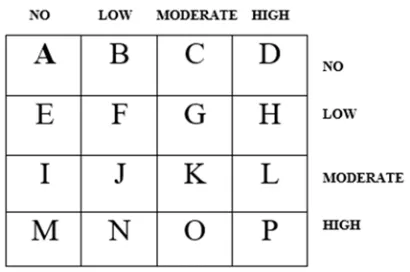
During the course of evaluating the predictive model, a number of metrics were used to quantify the model’s performance. In order to determine these metrics, four parameters must be identified from the results of predictions made by the classifier during model testing. These are: true positive (TP), true negative (TN), false positive (FP) and false negative (FP). True positives/negatives are correct classifications while false positives/negatives are incorrect classifications/misclassifications. These results are presented on confusion matrix-for this study the confusion matrix is a 4 x 4 owing to the three labels for the output class-risk of Thalassemia, namely: no, low, moderate and high risk.
Figure 2 shows the diagram of the confusion matrix that was used for evaluating the performance of the machine learning algorithms developed in this study.
Figure 2. Confusion matrix diagram for performance evaluation.
the cells across provides the number of actual cases in the training dataset while the sum of the columns provide the number of predicted cases in the training dataset. The cells located on the diagonal are the correct classifications (true positives/negatives) while other cells are the misclassifications/incorrect classifications (false positives/negatives). The performance metrics are thus defined as follows:
a. Sensitivity/True positive rate/Recall: is the proportion of actual cases that were correctly predicted.
j' ! Pk lFmFnFol (18)
j' ! _kV UFpFqF3p (19)
j' ! rksGtuXG wFxFvFav (20)
j' ! y zy {F|FWF.. (21)
b. False Positive rate/False alarm: is the proportion of actual cases that were incorrectly predicted. }' ! Pk ~•r]€•F~•rUFwF{‚€ƒ„…†‡„F~•rˆ1‰ˆ (22)
}' ! _kV ~•r6€F~•rUFwF{‚€ƒ„…†‡„F~•rˆ1‰ˆ (23)
}' ! rksGtuXG ~•r6€F~•rUFwF{]€•F~•rˆ1‰ˆ (24)
}' ! y zy ~•r6€F~•rUFwF{]€•F~•r‚€ƒ„…†‡„ (25)
where: Šf;Pk ‹ + Œ + • + Ž Šf;_kV J + } + • + " Šf;rksGtuXG • + ‘ + ’ + and Šf;y zy + + N + ' c. Precision: is the proportion of the predicted cases that were correctly predicted. ' “ Pk lFUFwF{l (26)
' “ _kV mFpFxF|p (27)
' “ rksGtuXG nFqFvFWv (28)
' “ y zy oF3FaF.. (29)
d. Accuracy: is the total number of correct classifications (positive and negative). ‹““f “M ~•r6€F~•r]€•lFpFvF.F~•r‚€ƒ„…†‡„F~•rˆ1‰ˆ (30)
4. Results and Discussion
4.1. Result of Data Identification and Collection
The analysis of the data containing information about the attributes for the 49 patients are shown in Tables 2 and 3. Table 2 shows the description of the nominal variables while Table 3 shows the distribution of the numeric variables. From the description shown in Table 2, there were more male than female respondents owing for a ratio of 1:1.08 for women to men. The number of patient records for the risk of Thalassemia consisted of 43.1% of respondents were without Thalassemia, 31.4% were with high risk, 15.7% with moderate risk while 9.8% were with low risk of Thalassemia. The results of the description of the variables showed that 1 patient data was missing for the values of employment status, 13 (25.5%) patient data was missing for the values of the description of their job type while 2 (3.9%) patient data was missing for the values of the academic qualification. The results further showed that about 57% of the patients were single while 37% were married with 6% separated; also about 31% of the patients were self-employed, 25% were employed, 35% were students while 6% were unemployed. The results further showed that 61% of the respondents were university graduates while 25% had secondary school education.
Based on the description of the risk factors, the results showed that majority of the patients had no family history of thalassemia owing for 55% of the patients, 70% of the patients had no enlarged spleen, 60% of the patients had no diabetes, and about 50% of patients had urine colour change while 62% had no parent carriers. The results show that majority of the patients had no spleen enlargement, diabetes nor parent carriers owing for about 60% of respondents while an equal number of patients had family history of thalassemia and urine colour change owing for about 50% of patients. From the description shown in Table 3, the analysis of the numeric datasets is presented showing the values of the minimum, maximum, mean and standard deviation of each numeric variable presented in the dataset. The variables presented are: weight, height and the body mass index of the patient data collected for this study.
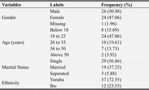
Table 2. Description of the nominal variables in the dataset.
Variables Labels Frequency (%)
Gender
Male 26 (50.98)
Female 24 (47.06)
Missing 1 (1.96)
Age (years)
Below 18 8 (15.69)
18 to 25 24 (47.06)
26 to 35 10 (19.61)
36 to 50 7 (13.73)
Above 50 2 (3.92)
Marital Status
Single 29 (56.86)
Married 19 (37.25)
Separated 3 (5.88)
Ethnicity Yoruba 37 (72.55)
Variables Labels Frequency (%)
Hausa 2 (3.92)
Employment Status
Employed 13 (25.49)
Self-employed 16 (31.37)
Unemployed 3 (5.88)
Student 18 (35.29)
Missing 1 (1.96)
Job Type
Nil 20 (39.22)
Engineer 4 (7.84)
Civil-servant 2 (3.92)
Doctor 1 (1.96)
Nurse 2 (3.92)
Clerical 4 (7.84)
Teacher 2 (3.92)
Trader 2 (3.92)
Artisan 1 (1.98)
missing 13 (25.49)
Academic Qualification
Primary 2 (3.92)
Secondary 13 (25.49)
University 31 (60.78)
Informal 3 (5.88)
Missing 2 (3.92)
Family History Yes 23 (45.10)
No 28 (54.90)
Spleen Enlargement Yes 15 (48.39)
No 36 (51.61)
Diabetes Present Yes 20 (39.22)
No 31 (60.78)
Urine Colour Change Yes 26 (50.98)
No 25 (49.02)
Parent Carriers Yes 19 (37.25)
No 32 (62.75)
Thalassemia Risk
No 22 (43.14)
Low 5 (9.80)
Moderate 8 (15.69)
High 16 (31.37)
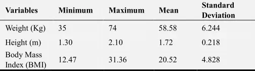
Table 3. Description of the numeric variables in the dataset.
Variables Minimum Maximum Mean Standard Deviation
Weight (Kg) 35 74 58.58 6.244
Height (m) 1.30 2.10 1.72 0.218
Body Mass
Index (BMI) 12.47 31.36 20.52 4.828
4.2. Results of Model Formulation and Simulation
Two different supervised machine learning algorithms were used to formulate the predictive model for the diagnosis of Thalassemia, namely: naïve Bayes’ and multi-layer perceptron. They were used to train the development of the prediction model using the dataset containing 51 patients’ risk factor records. The simulation of the prediction models was done using the Waikato Environment for Knowledge Analysis (WEKA). The C4.5 decision trees algorithm was implemented using the J48 decision trees algorithm available in the trees class and the naïve Bayes’ algorithm was implemented using the naïve Bayes’ classifier available in the Bayes class all available on the WEKA environment of classification tools. The models were trained using the 10-fold cross validation method which splits the dataset into 10
subsets of data-while 9 parts are used for training the remaining one is used for testing; this process is repeated until the remaining 9 parts take their turn for testing the model.
4.2.1. Results of the Naïve Bayes’ Classifier
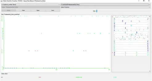
Following the simulation of the predictive model for classification of risk of Thalassemia using the naïve Bayes’ classifier, the evaluation of the performance of the model following validation using the 10-fold cross validation method was recorded. Figure 3 shows the screenshot of the results of the predictions made by the naïve Bayes’ classifier algorithm for the 51 instances of data collected from the patients considered for this study. The figures shows the correct and incorrect classifications made by the algorithm while Figure 4 shows the graphical plot of the predictions made by the naïve Bayes’ classifier algorithm on the dataset. In figure 4, each class of risk of Thalassemia is represented using a specific colour and each correct classification is represented with a star while each misclassification is represented as a square.
The results presented in figure 4 was used to evaluate the performance of the naïve Bayes’ classifier algorithm and thus, the confusion matrix determined. Figure 5 shows the confusion matrix that was used to interpret the results of the true positive and negative alongside the false positive and negatives of the validation results. The confusion matrix shown in figure 5 was used to evaluate the performance of the predictive model for classification of risk of Thalassemia. Based on the results presented in the confusion matrix with the naïve Bayes’ classifier used to train the predictive model developed using the training data via the 10-fold cross validation method, it was discovered that there were 48 (94.12%) correct classifications (22 for no, 5 for low, 7 for moderate and 14 for high risk-along the diagonal) and 3 (5.88%) incorrect classifications 1 moderate for low, 1 high for low and 1 high for moderate-along the vertical) as shown in figure 5. Hence, the predictive model for the risk of Thalassemia using the naïve Bayes’ classifier showed an accuracy of 94.12%.
Figure 3. Screenshot of naïve Bayes’ classifier results on dataset.
Figure 4. Screenshot of correct and incorrect classifications made by naïve Bayes’ classifier.
Table 4. Performance evaluation of the results of the naïve Bayes’ classifier.
Thalassemia Risk TP rate FP rate Precision Area under the ROC
No 1.000 0.034 0.957 0.997
Low 1.000 0.022 0.833 0.996
Moderate 0.875 0.023 0.875 0.983
High 0.875 0.000 1.000 0.996
Figure 5. Confusion matrix for the result of naïve Bayes’ classifier.
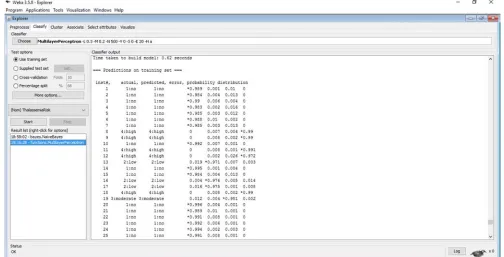
4.2.2. Results of the Multi-Layer Perceptron
Following the simulation of the predictive model for classification of risk of Thalassemia using the multi-layer perceptron, the evaluation of the performance of the model following validation using the 10-fold cross validation method was recorded. Figure 6 shows the screenshot of the results of the predictions made by the multi-layer perceptron algorithm for the 51 instances of data collected from the patients considered for this study. The figures shows the correct and incorrect classifications made by the algorithm while Figure 7 shows the graphical plot of the predictions made by the multi-layer perceptron algorithm on the dataset. In figure 7, each class of risk of Thalassemia is represented using a specific colour and each correct classification is represented with a star while each misclassification is represented as a square.
The results presented in figure 7 was used to evaluate the performance of the multi-layer perceptron algorithm and thus, the confusion matrix determined. Figure 8 shows the confusion matrix that was used to interpret the results of the true positive and negative alongside the false positive and negatives of the validation results. The confusion matrix shown in figure 8 was used to evaluate the performance of the predictive model for classification of risk of Thalassemia.
Based on the results presented in the confusion matrix with the multi-layer perceptron used to train the predictive model developed using the training data via the 10-fold cross validation method, it was discovered that there were 51 (100%) correct classifications (22 for no, 5 for low, 8 for moderate and 16 for high risk-along the diagonal) and no (0%) incorrect classifications as shown in figure 8. Hence, the predictive model for the risk of infertility using the multi-layer perceptron showed an accuracy of 100%.
From the information provided by the confusion matrix, it was discovered that all of the no, low, moderate and high risk cases were correctly classified. Table 5 shows the results of the evaluation of the performance of the multi-layer perceptron using the metrics. Based on the results presented for the multi-layer perceptron, the TP rate, FP rate and the precision all had values of 1 while the FP rate had a value of 0 for both the Yes and No cases. Therefore, the predictive model developed using the multi-layer perceptron was able to properly distinguish between the Yes and No cases available in the dataset presented for this study.
Figure 7. Screenshot of correct and incorrect classifications made by multi-layer perceptron.
Figure 8. Confusion matrix for the result of multi-layer perceptron.
The result of the performance evaluation of the machine learning algorithms are presented in Table 6 which presents the average values of each performance evaluation metrics considered for this study. For the naïve Bayes’ classifier algorithm based on the results presented in the confusion matrix presented in figure 6. The results showed that the TP rate which gave a description of the proportion of actual
cases that was correctly predicted was 0.938 which implied that 93.8% of the actual cases were correctly predicted; the FP rate which gave a description of the proportion of actual cases misclassified was 0.011 which implied that 1.1% of actual cases were misclassified while the precision which gave a description of the proportion of predictions that were correctly classified was 0.916 which implied that 91.6% of the predictions made by the classifier were correct. For the multi-layer perceptron algorithm based on the results presented in the confusion matrix presented in figure 8.
The results showed that the TP rate which gave a description of the proportion of actual cases that was correctly predicted was 1 which implied that 100% of the actual cases were correctly predicted; the FP rate which gave a description of the proportion of actual cases misclassified was 0 which implied that 0% of actual cases were misclassified while the precision which gave a description of the proportion of predictions that were correctly classified was 1 which implied that 100% of the predictions made by the classifier were correct.
Table 5. Performance evaluation of the results of the multi-layer perceptron.
Class TP rate FP rate Precision Area under the ROC
No 1.000 0.000 1.000 1.000
Low 1.000 0.000 1.000 1.000
Moderate 1.000 0.000 1.000 1.000
High 1.000 0.000 1.000 1.000
Average 1.000 0.000 1.000 1.000
In general, multi-layer perceptron algorithm were able to classify the performance of students by graduation better than the naïve Bayes’ classifier algorithm. The multi-layer
Table 6. Summary of the results of performance evaluation for the machine learning algorithms selected.
Machine Learning Algorithm Used
Performance Evaluation Metrics
Correct Classification (out of 51) Accuracy (%) TP rate (recall / sensitivity) FP rate (false positive) Precision
Naïve Bayes’ Classifier 48 94.12 0.938 0.011 0.916
Multi-Layer Perceptron 51 100.00 0.000 1.000 1.000
5. Conclusion
This study focused on the development of a prediction model using identified classification factors in order to classify the classification of risk of Thalassemia in selected patients for this study. Historical dataset on the distribution of the classification of risk of Thalassemia among patients was collected using questionnaires following the identification of associated classification factors of risk of Thalassemia from expert medical practitioners.
The dataset containing information about the classification factors identified and collected from the patients was used to formulate predictive model for the classification of risk of Thalassemia using 2 machine learning algorithm-naïve Bayes’ classifier and the multi-layer perceptron. The predictive model development using the decision trees algorithm was formulated and simulated using the WEKA software. The predictive model developed using the multi-layer perceptron and naïve Bayes’ classifier algorithms were compared in order to determine the algorithm with the best performance.
In this paper, the development of a predictive model for predicting the diagnoses of Thalassemia given the values of risk factors was developed using dataset collected from patients in a hospital in the south-western part of Nigeria. After the process of data collection and pre-processing, two supervised machine learning algorithms were used to develop the predictive model for the diagnosis of Thalassemia using the historical dataset from which the training and testing dataset was collected. The 10-fold cross validation method was used to train the predictive model developed using the machine learning algorithms and the performance of the models evaluated. The multi-layer perceptron algorithm proved to be an effective algorithm for predicting the diagnosis of Thalassemia in Nigerian patients.
References
[1] Gretchen Holm and Kristeen Cherney (2017). Thalassemia. Available from https://www.healthline.com/health/thalassemia [Access on 7th August, 2018].
[2] World Health Organization (WHO) (1968). Nutritional anemia: report of a WHO Scientific Group. Geneva, Switzerland: World Health Organization.
[3] World Health Organization (2011). WHO Vitamin and Mineral Nutrition. Geneva, Switzerland: World Health Organization.
[4] Ivoke, N., Eyo, J. E., Ivoke, O. N., Nwani, C. D., Odii, E. C.,
Asogwa, C. N., Ekeh, F. N. and Atama, C. I. (2013). Anaemia Prevalence and Associated Factors among Women Attending Antenatal Clinics in South-Western Ebonyi State, Nigeria. International Journal of Medicine and Medical Sciences 46 (4): 1354-1359.
[5] Osungbade, K. O. and Oladunjoye, A. O. (2012). Preventive treatments of iron deficiency Anaemia in pregnancy: a review of their effectiveness and implications for health system strengthening. Journal of Pregnancy 2012: 1-7.
[6] Siteti, M. C., Namasaka, S. D., Ariya, O. P., Injete, S. D. and Wanyonyi, W. A. (2014). Anaemia in Pregnancy: Prevalence and Possible Risk Factors in Kakamega County, Kenya. Science Journal of Public Health 2 (3): 216-222.
[7] World Health Organization (WHO) (1992). The prevalence of Anaemia in women; a tabulation of available information. Geneva: World Health Organization.
[8] Kaur, P., Singh, M. and Josan, G. (2015). Classification and Prediction Based Data Mining Algorithms to Predict Slow Learners in Education Sector. Procedia Computer Science 57: 500-508.
[9] Kishore, C. R., Rao, K. P. and Murthy, G. (2015). Performance Evaluation of Entropy and Gini Using Threaded and Non-Threaded ID3 on Anaemia Dataset. Life 6 (10): 10-12.
[10] Chuang L-Y, Wu K-C, Chang H-W, Yang C-H (2011) Support vector machine-based prediction for oral cancer using four snps in DNA repair genes. In: Proceedings of the international multiconference of engineers and computer scientists, March 16–18 2011.
[11] Hu, Z. Fan, C., Oh, D. S., Marron, J. S., He, X., Qaqish, B. F., Livasy, C. and Carey, L. A. (2006). The molecular portraits of breast tumors are conserved across microarray platforms. BMC Genomics 7: 96-107.
[12] Huang, C.-L., Liao, H.-C. and Chen, M.-C. (2008). Prediction Model Building and Feature Selection with Support Vector Machines in Cancer Diagnosis. Journal of Expert Systems with Applications 34 (1): 578-587.
[13] Curiac, D. I., Vasile, G., Banias, O., Volosencu, C and Albu, A. (2009). Bayesian Network Model for Diagnosis of Psychiatric Diseases. In Proceedings of the ITI 2009 31st International Conference on Information Technology Interfaces held on June 22-25, 2009 at Cavtat, Croatia: 61-66. [14] Amin, N. and Habib, A. (2015). Conparison of Different
Classification Technoiques Using WEKA for Hematological Data. American Journal of Engineering Research (AJER) 4 (3): 55-61.