ORIGINAL ARTICLE
Ali Awaludin · Takuro Hirai · Toshiro Hayashikawa Yoshihisa Sasaki · Akio Oikawa
One-year stress relaxation of timber joints assembled with
pretensioned bolts
Abstract In our previous study, great increases of hyster-etic damping and initial slip resistance of timber joints were attained by applying axial pretension to the steel fasteners. To evaluate the effectiveness of this method, 1-year stress-relaxation measurement was carried out. Nine prestressed joints were prepared and three of them were restressed after 3 and then 6 months after the initial prestressing. All joints were exposed to indoor conditions, and relaxation of the pretension was regularly measured from time-dependent decreases of axial strain of the bolts. After mea-surement, the joints were subjected to cyclic and monotonic loading tests until failure. The average ratio of residual stress to the initial prestress after 1 year was about 0.23 and 0.66, respectively, for joints without restressing and those with restressing. A simulated stress-relaxation curve devel-oped from the four-element relaxation model predicted 3% of the initial stress after 5 years. Without a regular restress-ing program, the initial prestressrestress-ing effect therefore must be considered negligible. However, about 20% of the pre-stress level can be reasonably assumed if repre-stressing is carried out annually. This small residual stress was found to introduce suffi cient frictional damping to signifi cantly increase the equivalent viscous damping ratio of the joints.
Key words Bolted joint · Frictional damping · Pretension · Residual stress · Stress relaxation
A. Awaludin1 · T. Hayashikawa · A. Oikawa
Graduate School of Engineering, Hokkaido University, Sapporo 060-8628, Japan
T. Hirai (*) · Y. Sasaki
Graduate School of Agriculture, Hokkaido University, Kita 9 Nishi 9, Kita-ku, Sapporo 060-8589, Japan
Tel. +81-11-706-2591; Fax +81-11-716-0879 e-mail: hirai@for.agr.hokudai.ac.jp
Present address:
1 Civil and Environmental Engineering Department, Gadjah Mada University, Yogyakarta 55281, Indonesia
Part of this study was presented at the 10th World Conference on Timber Engineering, Miyazaki, June 2008
Introduction
Seismic performance of timber constructions (wooden buildings etc.) principally depends on the dynamic proper-ties of timber joints. Various techniques to improve the dynamic properties of timber joints have been reported by previous studies.1–5 All the techniques have been focused on the increase of hysteretic damping, ductility, or fatigue resistance of the bolted joints. In the authors’ previous work,5
the effect of pretension force applied to the steel fasteners of moment-resisting joints was examined, and this showed great increases of initial rotational stiffness and hysteretic damping of the joints. These signifi cant improve-ments, however, would decrease as the given prestress relaxed due to the viscoelastic nature of timber.6,7 Detailed information about the effect of stress relaxation on hyster-etic damping of the prestressed (bolted timber) joints is presented in this study. The joints were exposed to indoor environmental conditions for 1 year after initial prestressing and their stress relaxations were continuously measured throughout the test. Their hysteretic damping obtained from the cyclic tests, after completing the relaxation mea-surement, was compared with the hysteretic damping of the prestressed joints that experienced no relaxation in our earlier study.5
Stress-relaxation model
A four-element relaxation model shown in Fig. 1 was used to simulate the stress-relaxation behavior of prestressed bolted timber joints.8
The governing equation of this model is expressed as
k k N k r k r dN dt r r
d N dt
1 2 1 2 2 1 1 2
2
2 0
+( + ) + = (1)
where N is the bearing force resulting from the fastener pretension forces. The constant parameters of Eq. 1 can be evaluated by wood creep tests, in principle, because Received: April 21, 2008 / Accepted: August 4, 2008 / Published online: October 15, 2008
stress relaxation or creep deformation of timber joints is completely infl uenced by viscoelastic properties of wood members. The viscoelastic properties of some wood species, which can be used to understand the time-dependent behav-ior of timber joints, have been intensively examined via creep test in some previous studies.9–11
By equating the coeffi cients of the governing equation of creep phenomenon described by Bodig and Jayne8
with those in Eq. 1, the constants of Eq. 1 can be expressed as
r r
r
k C C k k r k
2
2
1 2
2
2
22
1
4 2
4
= + ( ) − =
= − − =
μ μ μ μ μ μ
μ μ μ μ
v v v k v k
v k e k
v k
2
; ;
; kk k
k e k
2
(2)
where
C=r k2( k vμ +ke vμ +ke kμ ) (3) In the equations, ke and mv are the elastic spring constant and the viscous damper constant, respectively, of a Maxwell body, while kk and mk are the elastic spring constant and
viscous damper constant, respectively, of a Kelvin body. The solution of Eq. 1 is given by two negative exponential functions as
N N e N e
k rt
k r t = 1 − + 2 −
1 1
2
2 (4)
Stress relaxation is a result of compound action among the viscoelastic constants of Maxwell and Kelvin bodies, which were reported to be dependent upon wood species and test conditions.10,11
Therefore, to substitute all the constants at the same time using creep test results of some previous studies may lead to disagreement between the predicted and experimental results. Considering this diffi -culty of direct application of previous information of visco-elastic properties of wood to the simulation of the stress relaxation of timber joints, only the initial values of the constants, kk and mk, of the Kelvin body were adopted from the results of creep tests of Douglas fi r under constant envi-ronmental condition [22.8°C, 50% relative humidity (RH)].10 After that, the constants of the Maxwell body were itera-tively selected to fi t the experimental stress–relaxation curves. Because the main objective of this study is to obtain a simulation curve that well fi ts the observed one, determin-ing in advance either the constants of the Kelvin body or the Maxwell body is of no particular interest. In this curve-fi tting method, the viscous constant mv was linearly related with the viscous constant mk through the constant l and the spring constant ke was linearly related with the spring constant kk by the constant h. The constant parameters of relaxation that are obtained through this curve fi tting, however, may not guarantee that the same constants will be applicable when test conditions are changed. Simulated curves for 1 year of stress relaxation with different values of l and h are shown in Fig. 2. N1 and N2, which indicate the short-term and long-term relaxation, were arbitrarily set to 0.7N and 0.3N, respectively. In the actual curve fi tting, however, N1 and N2 must also be determined by some trials.
(a) (b)
N
N ke
kk
μk
μv
Fig. 1a, b. Stress-relaxation model. a Cross section of the prestressed joint, and b four-element relaxation model
0.0 0.2 0.4 0.6 0.8 1.0
0 60 120 180 240 300 360
Elapsed time (days) η= 0.5
η
= 10η
= 5η
= 2.5η
= 1.5λ
= 500.0 0.2 0.4 0.6 0.8 1.0
0 60 120 180 240 300 360
Elapsed time (days)
λ
= 4λ
= 7λ
= 10λ
= 20λ
= 50η
= 0.5ρ
Stress ratio (
)
(a) (b)
A higher value of l in Fig. 2a gives less long-term relax-ation. On the other hand, a higher value of h gives more rapid relaxation at the initial stage (see Fig. 2b).
Stress-relaxation measurement
Nine prestressed bolted timber joints with spruce–pine–fi r lumber as shown in Fig. 3 were exposed to indoor condi-tions for 1 year. Moisture content and specifi c gravity of the wood at initial prestressing were 13% and 0.38, respectively. Figure 4 shows the geometry of the joint where 4-mm-thick steel plates and 12-mm-diameter bolts were used as in our previous study.5
In monotonic tension tests on three repli-cates, the bolts were found to have an ultimate tensile strength of 440 MPa and 0.2% offset yield strength of 386 MPa. Axial pretension force of 20 kN per fastener, which was applied using a torque wrench device, yielded a prestress level of 1.6 MPa or 90% of the allowable long-term edge-bearing stress of spruce species.12
This prestress level was calculated by considering the total pretension
forces and the contact area between the wood member and the steel plate. Three of the nine specimens were restressed twice after 3 months and 6 months after the initial prestress-ing, while the other six specimens were not restressed throughout the 1-year measurement. The given axial pre-tension force during the fi rst or second restressing was made as close as possible to the pretension force applied at the initial prestressing.
The relaxation of pretension force given to the bolts was measured from the time-dependent decrease of axial strain of the bolts in the following way. A strain gauge was inserted into a hole of 2 mm in diameter drilled in the longitudinal direction of the bolt. The strains were measured for 2 bolts of each joint specimen assembled with 12 bolts (see Fig. 4). The fastener strains were recorded regularly every 6 h throughout the test, but more often observation was carried out in the fi rst 5 days to consider the possibility of high immediate relaxation. The relative humidity inside the testing laboratory at 60 days after the beginning of the test varied in a wide range because heating was used in daytime due to the fall and winter seasons. During this period, the relative humidity could reach a minimum of 20% and a maximum of 60%. After the cold season, the relative humid-ity was relatively stable from a minimum of 60% to a maximum of 80%. Because relative humidity has great infl uence on the relaxation curve, a different curve would be obtained for measurements started at different times of the year.
Experimental relaxation curves shown in Fig. 5 show that stress relaxation occurs rapidly for the initial 120 days but it becomes very slow after that term. The average stress ratio r, defi ned as the ratio of the residual stress to the initial prestress, reached a constant value of 0.23 at 1 year after initial prestressing. In the case of restressed joints, the average residual stress after 1 year was found to be 0.66 as shown in Fig. 6. Although the stress level was identical for initial prestressing and restressing, the residual stress ratios for the same duration, r1 for the prestressing, r2 for the fi rst restressing. and r3 for the second restressing were in the order of r3>r2>r1 as shown in Fig. 6. This indicates that restressing reduces the amount of stress relaxation.
The experimental stress-relaxation curves showed that the stress fl uctuated in a wide range 60 days after initial prestressing. This phenomenon, which must have been the result of the combined effects of mechanosorptive creep and swelling and shrinkage13,14
caused by large variation of relative humidity, continued up to about 240 days. In the fi rst 60 days of observation, some stresses of the fasteners recovered as shown in Fig. 5. Because the effect of rela-tive humidity variation in this time interval is a minimum, this particular situation might indicate that the strain relaxation rates in each fastener of the joints were different from each other. As the strains of fasteners around the one equipped with the strain gauge relax, wood beneath the fastener with the strain gauge expands laterally, induc-ing some axial stresses to the fastener with the strain gauge. This comes from the relatively thin steel plate of the joint that causes different local relaxation behavior of the wood member. This behavior cannot be examined in one-Fig. 3. Stress-relaxation measurement
280 mm
270 mm CL
6φ12-mm bolt
Symmetry
Timber 4-mm steel plate
100 mm Bolt with strain-gauge
2-mm hole Strain-gauge
dimensional (1-D) models, which are developed based on an assumption that the joint is uniformly compressed by one single rod, such as the four-element relaxation model adopted in this study.
After some trials, a simulated stress-relaxation curve shown in Fig. 5 was determined as
ρ =0 7. e−45+0 3. e−810
t t
(5)
by substituting l = 4, h = 0.75, N1 = 0.7N, N2 = 0.3N, kk= 0.5 GPa, and mk= 6 × 10
4
GPa min into Eq. 4 where t is time in days since the initial prestressing. While the stress-relaxation curve after restressing (see Fig. 6) can be fi tted only if the elastic spring constant and viscous damper con-stant of both Kelvin and Maxwell bodies are increased. This is because the observed relaxation curves of the prestressed joints with restressing have smaller short-term relaxation and lower long-term relaxation rates than those of the pre-stressed joints without restressing. A curve that well fi tted the observed time-dependent relaxation after the second restressing was expressed by
ρ =0 3. e−24+0 7. e−4971
t t
(6)
Stress ratios of the joints some years after the initial pre-stressing can be roughly estimated by utilizing the simulated relaxation curves. For instance, the stress ratios of the joints without restressing after 5 and 10 years were 0.03 and 0.003, respectively. For joints with restressing, these ratios were 0.40 and 0.23, respectively. It can be concluded that a much higher residual stress can be expected when the joint is fre-quently restressed in the initial years.
Apart from the stress-relaxation curve governed by Eq. 4, an attempt to predict the stress ratio was carried out using Eq. 7
ρ = −c c
(
−e−c t)
−c t1 2 1 3 4 (7)
where c1, c2, c3, and c4 are empirical constants, and t is time in days since the initial prestressing. The equation was
0.0 0.2 0.4 0.6 0.8 1.0
0 60 120 180 240 300 360
Elapsed time, t, (day)
Stress ratio
(
ρ)
Eq. 5 Eq. 7
0.0 0.2 0.4 0.6 0.8 1.0
0 60 120 180 240 300 360
Elapsed time, t, (day)
Stress ratio
(
ρ)
Eq. 5
Eq. 7
0.0 0.2 0.4 0.6 0.8 1.0
0 60 120 180 240 300 360
Stress ratio
(
ρ)
Elapsed time, t, (day)
Eq. 5 Eq. 7
Fig. 5. Experimental 1-year stress-relaxation curves of prestressed joints without restressing
0.0 0.2 0.4 0.6 0.8 1.0
0 60 120 180 240 300 360
Stress ratio
(
ρ
)
Elapsed time, t, (day)
ρ1 ρ2 ρ3
obtained, with slight changes, from the most often used empirical functions to describe the primary and secondary creep behavior given by Bodig and Jayne.8
Good agreement between the experimental stress-relaxation curve and Eq. 7 as shown in Fig. 5 was found by letting c1= 1.0, c2= 0.80, c3 = 0.015, and c4= 8 × 10−
5
. As a result, Eq. 7 showed that the stress ratios after 5 years would be 0.05 and complete stress relaxation will take place at 7 years after the initial pre-stressing. It is obvious that the long-term relaxation of the prestressed joints is simulated more rapidly by Eq. 7 than that by Eq. 5. Both prediction curves, which are governed by Eq. 5 and Eq. 7, indicate that the residual stress will be equal to zero after several years, although a nonzero reten-tion stress as the fi nal residual stress might be observed in the experimental curves (see Fig. 5).
Hysteretic damping
Just after completing the 1-year stress-relaxation measure-ment, all the joints were subjected to quasi-static cyclic loading tests in the same way as in the authors’ previous work.5
A displacement-controlled loading was used in the cyclic test and the reversed load was performed continu-ously within six rotation levels. The cyclic load was carried out up to a rotation level of 0.0148 radians or about 10% of the ultimate rotation of the nonprestressed joints. Figure 7 shows typical hysteretic loops of the joints with different test conditions adopted in this study where the cyclic load was repeated fi ve times at each rotation level. To evaluate the infl uence of test conditions on hysteretic damping of the joints, fractional constants
r E
E
1=
Dr
Dn (8)
and
r E E
E E
2= −
−
Dr Dn
Dp Dn (9)
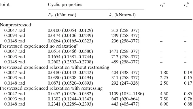
were introduced where EDn is hysteretic damping of the nonprestressed joint, EDp is hysteretic damping of the pre-stressed joint that experienced no relaxation, and EDr is hysteretic damping of the prestressed joint that experienced relaxation. Experimental hysteretic damping (ED) and rotational stiffness (kr) of the joints along with their frac-tional constants at three different cyclic rotation levels are presented in Table 1. These cyclic properties were eval-uated using the hysteresis loop of the last cycle. Although the pretension force decreased considerably after 1 year, the hysteretic damping of the joints (see Fig. 7a) was still much higher than that of the nonprestressed joints (see Fig. 7b), as indicated by the constant r1 in Table 1. More-over, the constant r1 of the joints with or without restressing increased as the cyclic rotation level was increased. This is because the additional frictional damping due to the sec-ondary axial force was easier to be effectively developed in the prestressed joints than that in the nonprestressed joints.
-12 -8 -4 0 4 8 12
-0.02 -0.01 0.00 0.01 0.02
Rotation (rad)
Moment (kNm)
(a)
-12 -8 -4 0 4 8 12
-0.02 -0.01 0.00 0.01 0.02
Rotation (rad)
Moment (kNm)
(b)
-12 -8 -4 0 4 8 12
-0.02 -0.01 0.00 0.01 0.02
Moment (kNm)
Rotation (rad)
(c)
-12 -8 -4 0 4 8 12
-0.02 -0.01 0.00 0.01 0.02
Rotation (rad)
Moment (kNm)
(d)
Fractional constant r2 indicates the percentage of remain-ing hysteretic dampremain-ing contributed by the fastener preten-sion. This constant is equivalent to the stress ratio r because frictional damping or the hysteretic damping contributed by the fastener pretension is proportional to the residual stress. After being exposed to indoor conditions for 1 year, hyster-etic damping or the area enclosed by a hysterhyster-etic loop of the prestressed joints (see Fig. 7a) became smaller than the hysteretic damping of the prestressed joints that experi-enced no relaxation (see Fig. 7c). The values of the frac-tional constant r2 of the joints without restressing were 0.19, 0.15, and 0.17 at the three rotation levels (see Table 1). These ratios, which indicate the hysteretic damping contrib-uted by the pretension force, were less than the average stress ratio obtained from the fastener strain measurement (0.23). Hysteretic damping of the prestressed joint with restressing shown in Fig. 7d is less than the hysteretic damping of the prestressed joint that experienced no relax-ation (see Fig. 7c). The r2 values of these prestressed joints were found to be 0.85, 0.76, and 0.88 at the three rotation levels as shown in Table 1. Fractional constant r2 of the joints at any cyclic rotation level was relatively higher than the stress ratio observed from the fastener strain measure-ment, which was 0.66. Increasing the number of bolts equipped with a strain gauge may reduce this discrepancy.
After completing the cyclic test, all of the joint specimens were loaded monotonically until failure. The maximum moment resistance was 14.38 kNm for the joints with restressing and 13.87 kNm for the joints without restressing. This maximum moment resistance is intermediate between the moment resistance of the nonprestressed joints and that of the prestressed joints tested in our previous study5 (maximum moment resistances of the nonprestressed and prestressed joints that experienced no relaxation were 13.42 kNm and 14.87 kNm, respectively). A slight
differ-ence in moment resistance among these joints indicates that the prestressing effect is relatively small at the ultimate condition. In nonprestressed joints or joints with low pre-stress level, frictional resistance caused by the secondary fastener axial force leads to a great increase in the ultimate resistance. The average sliding moment resistances at interlayer slip occurrence were found to be 3.87 kNm and 0.87 kNm for the joints with and without restressing, respec-tively. Therefore, these moment resistances were about 0.81 and 0.18 times the sliding moment resistance of the pre-stressed joints that experienced no relaxation in our previ-ous study,5
which was 4.78 kNm. These sliding resistance ratios were almost the same as the average percentages of the remaining hysteretic damping contributed by the fas-tener pretension, which were indicated by the constant r2.
Hysteretic damping of the prestressed joint after some years can be attained by adding the rectangular hysteretic damping due to frictional resistance into the hysteretic damping of the nonprestressed joint. As a result, hysteretic damping and rotational stiffness of the prestressed joints after some years may follow these expressions
EDr( )t =EDn+ρ( )t E
(
Dp−EDn)
(10) krr( )t =krn+ρ( )t k(
rp−krn)
(11) where r(t) is given by Eq. 5 or Eq. 6, krn is rotational stiff-ness of the nonprestressed joint, krp is rotational stiffness of the prestressed joint that experienced no relaxation, and krr is rotational stiffness of the prestressed joint that experi-enced relaxation. The effects of relaxation on the seismic performance of prestressed joints, which are characterized by hysteretic damping reduction and stiffness degradation, can be unifi ed through evaluation of the equivalent viscous damping ratio (zeq).15
The equivalent viscous damping ratio of the joint after some years is formulated as follows Table 1. Cyclic properties of timber joints with some different test conditions
Joint Cyclic properties r1
a r
2 b
ED (kNm rad) kr (kNm/rad)
Nonprestressedc
0.0047 rad 0.0100 (0.0054–0.0129) 313 (258–377) – – 0.0093 rad 0.0174 (0.0106–0.0239) 239 (258–377) – – 0.0148 rad 0.0264 (0.0165–0.0323) 236 (258–377) – – Prestressed experienced no relaxationc
0.0047 rad 0.0514 (0.0466–0.0580) 1471 (258–377) – – 0.0093 rad 0.1654 (0.1581–0.1744) 713 (258–377) – – 0.0148 rad 0.2603 (0.2503–0.2708) 489 (258–377) – – Prestressed experienced relaxation without restressing
0.0047 rad 0.0180 (0.0143–0.0242) 404 (338–477) 1.80 0.19 0.0093 rad 0.0390 (0.0308–0.0494) 311 (258–377) 2.25 0.15 0.0148 rad 0.0671 (0.0520–0.0893) 292 (247–326) 2.50 0.17 Prestressed experienced relaxation with restressing
0.0047 rad 0.0452 (0.0376–0.0582) 1109 (1054–1186) 4.50 0.85 0.0093 rad 0.1302 (0.1244–0.1343) 647 (620–664) 7.50 0.76 0.0148 rad 0.2341 (0.2289–0.2393) 443 (405–477) 8.90 0.88
Values in parentheses are minimum and maximum values
ED, Hysteretic damping; kr, rotational stiffness a r
1 = EDr/EDn b r
Table 2. Predicted equivalent viscous damping (zeq) of the prestressed joint without restressing at 0.0148 rad of rotation
Elapsed time (years) r EDr (kNm rad) krr (kNm/rad) zeq
0 1.00 0.260 489 0.39
1 0.19 0.071 284 0.18
2 0.12 0.055 266 0.15
5 0.03 0.034 244 0.10
10 0.00 0.027 236 0.08
r, Stress ratio predicted by Eq. 5; EDr, hysteretic damping evaluated by Eq. 10; krr, rotational stiffness estimated by Eq. 11
ζ
π π θ
eq Dr
p
Dr
rr
t E t
E t
E t
k t ( )= ( )
( ) ≅ ( )( )
1 4
1 4 0 5 2
. (12)
where Ep(t) is the potential energy. Evaluation of the equiv-alent viscous damping ratio of the prestressed joint without restressing at cyclic rotation level q= 0.0148 rad is presented in Table 2. The numerical values of EDn= 0.0264 kNm rad, EDp= 0.2603 kNm rad, krn= 236 kNm/rad, and krp= 489 kNm/ rad, which were reported earlier,5
were used. Table 2 shows that the equivalent viscous damping ratio decreased rapidly during the fi rst year after the initial prestressing. The remaining prestress after 1 year of relaxation gave an equiv-alent viscous damping ratio of 0.18, which is about 125% higher than that of the nonprestressed joint. After 5 years, the prestressing effect on cyclic performance of the joint was negligible because the equivalent viscous damping ratio of the prestressed joint was equal to the ratio of the non-prestressed joint.
In bolted timber connections, secondary axial forces due to bending deformation of fasteners contribute to the maximum resistance, which is known as the rope effect.16,17 Additional resistance described by this effect includes the formation of adverse bending moment of the fasteners, embedding resistance of the side member, and friction between the joint members. Although the prestress decreases or fades away after some years, the remaining slight stress might keep the main and side members of the joints in contact with each other. This contact develops the effect of secondary fastener axial force at the early stage of joint deformation, which results in effective frictional damping. To obtain an appropriate estimation of this sup-plementary advantage, further experimental or analytical study is required.
Without a regular restressing program, initial prestress-ing effects is ineffective in practice because the prestress completely diminishes after some years. If restressing is regularly carried out, for example, annually, about 20% of initial prestressing level can be practically assumed. About the same residual stress can also be expected if the joint is specially restressed every 10 years in which each restressing is conducted three times with a 3-month interval. The latter method is probably more benefi cial than the fi rst one because it reduces labor or cost and minimizes the distrac-tion to existing structures. In follow-up, the restressing schedule would be optimized by accumulating the informa-tion of stress-relaxainforma-tion curves for various prestress levels and intervals. The use of Belleville disk springs as an
alter-native to increase the residual stress has been proposed.18 These disk springs work as anchorage plates to reduce the effective stiffness of the prestressing system.
Conclusions
This study reported observation of stress relaxation of pre-stressed timber joints via strain measurement of their steel fasteners. After being exposed to indoor conditions for about 1 year after the initial prestressing, the average ratio of residual stress to the original prestress in joints without restressing was 0.23. This ratio increased to 0.66 when the joints were restressed twice after 3 months and 6 months. Although a large decrease of pretension force was found due to relaxation, the hysteretic damping of the joints without restressing was still relatively higher than that of the nonprestressed joints. Signifi cant frictional damping from frictional resistance among the joint components was found to be proportional to the fastener residual stress. Based on the simulated stress-relaxation curve, which was developed according to the four-element relaxation model, residual stress of the joints is negligible after 5 years if restressing is not applied. However, about 20% of the prestress level can be reasonably expected when restressing is carried out annually. This small residual stress has a sig-nifi cant effect on the cyclic performances of the joints, increasing the equivalent viscous damping ratio from 0.08 to 0.18.
Acknowledgments The fi rst author (A. Awaludin) thanks the Japan International Cooperation Agency (JICA) for the educational scholar-ship provided through AUN/SEED-Net program.
References
1. Leijten AJM, Ruxton S, Prion H, Lam F (2006) Reversed-cyclic behavior of a novel heavy timber tube connection. J Struct Eng 132:1314–1319
2. Dinehart DW, Blasetti AS, Shenton HW (2008) Experimental cyclic performance of viscoelastic gypsum connection and shear wall. J Struct Eng 134:87–95
3. Blass HJ, Schmid M, Litze H, Wagner B (2000) Nail plate rein-forced joints with dowel-type fasteners. Proceedings of the World Conference on Timber Engineering, Whistler, Canada, July 31– August 3, Paper 8.6.4
Conference on Timber Engineering, Portland, USA, August 6–10, Paper 3.4.4
5. Awaludin A, Hirai T, Toshiro T, Sasaki Y, Oikawa A (2008) Effects of pretension in bolts on hysteretic responses of moment-carrying timber joints. J Wood Sci 54:114–120
6. Manrique RE (1969) Stress relaxation of wood at several levels of strain. Wood Sci Technol 3:49–73
7. Quenneville P, Dalen KV (1994) Relaxation behaviour of pre-stressed wood assemblies. Part 1: experimental study. Can J Civ Eng 21:736–743
8. Bodig J, Jayne BA (1982) Mechanics of wood and wood compos-ites. Van Nostrand Reinhold, New York, pp 216–221
9. Fridley KJ, Tang RC, Soltis LA (1992) Load duration effects in structural lumber: strain energy approach. J Struct Eng 118: 2351–2369
10. Fridley KJ, Tang RC, Soltis LA (1992) Creep behavior model for structural lumber. J Struct Eng 118:2261–2277
11. Yazdani N, Johnson E, Duwadi S (2004) Creep effect in structural composite lumber for bridge applications. J Bridge Eng 9:87– 94
12. Architecture Institute of Japan (2006) Standard for structural design of timber structures. Architecture Institute of Japan, Tokyo, pp 13–14, 400
13. Alfthan J, Gudmundson P, Ostlund S (2002) A micro-mechanical model for mechano-sorptive creep in paper. J Pulp Pap Sci 28:98–104
14. van der Put TACM (1988) Theoretical explanation of mechano-sorptive effect in wood. Wood Fiber Sci 21:219–230
15. Chopra AK (2001) Dynamics of structures: theory and applications to earthquake engineering. Prentice Hall, Upper Saddle River, pp 99–104
16. Hirai T (1991) Analysis of the lateral resistance of bolt joints and drift-pin joints in timber II: numerical analysis applying the theory of a beam on an elastic foundation (in Japanese). Mokuzai Gak-kaishi 37:1017–1025
17. Nishiyama N, Ando N (2003) Analysis of load–slip characteristics of nailed wood joints: application of a two dimensional geometric nonlinear analysis. J Wood Sci 49:505–512