O R I G I N A L P A P E R
Open Access
Compositional data techniques for the
analysis of the container traffic share in a
multi-port region
M. Grifoll
*, M. I. Ortego and J. J. Egozcue
Abstract
The statistical techniques based on compositional data are applied to investigate the evolution of the traffic share of the container throughput in a multi-port system. Compositional vectors are those which contain relative information of parts of some whole. The application of conventional statistical techniques to compositional data may lead to erroneous conclusions and spurious correlations. Therefore, compositional data (CoDa) should be treated taking into account their own mathematical structure. The so-called log-ratio approach provides a set of transformations that allow to apply conventional statistical techniques to the transformed compositional data samples. Thus, the objective of this paper is double. As a first stage it aims to introduce the CoDa formalism and highlight its potentiality in the port container throughput analysis as example of transport system providing an applied example: the container
throughput evolution in the Spanish Mediterranean Ports system during the period 1976–2015. Second, based on the previous analysis, the aim is to characterize the container throughput in SpanishMed ports and its temporal evolution. The CoDa analysis clarifies the interpretation and data association of the container traffic throughput evolution in function of some selected change points: boom of containerization in 1990s and 2008 crisis. This contribution proves that the CoDa methodology is useful to investigate the complexity of the transport disciplines in order to understand and to manage the spatial integration that results from the movement of people and freight.
Keywords: Multi-port system, Traffic share, Container throughput, Compositional data, SpanishMed
1 Introduction
Transport disciplines are motivated to explain the spa-tial integration that result from the movement of people and freight from one place to another. From a descriptive point of view, several contributions seek to understand the spatial organization of mobility considering its attributes and constraints (e.g. [6–9, 15, 17, 22, 25, 26, 30, 32]). Terminals, modes and networks are the basis of com-plex systems under constant evolution influenced by the geo-spatial economy development (with private and public agents), growth of infrastructures and physical restrictions. The development of methodological strate-gies has allowed to describe and explain transport systems
*Correspondence:[email protected]
Department of Civil and Environmental Engineering, Universitat Politècnica de Catalunya (UPC-BarcelonaTech), C/Jordi Girona, 1-3, 08028, Barcelona, Spain
according to its evident complexity. This contribution pursues the introduction of Compositional Data (CoDa) methodology in the transport system analysis using as example the evolution of the container traffic in the Span-ish Mediterranean Sea (SpanSpan-ishMed) port system.
Containerization plays an important role in the mar-itime transport and in the global economy growth. Since the first wave of containerization (1970s), the global con-tainer traffic has been reformulated seeking economy of scales and more efficient distribution systems (e.g. hub-and-spoke model or transshipment activity). In this sense, the container throughput share of ports has evolved at the same time that the industrial regions and global trade have shifted. Also, shippers and logistic providers select a chain where the port is merely a node [25]. In the recent years, new container ports have emerged as relevant actors in container throughput at the same time that other ports have gradually lost their relevance. An S-shaped curve has been observed in the traffic evolution of world ports
Grifollet al. European Transport Research Review (2019) 11:12 Page 2 of 15
(increasing rapidly in the late 1970s and slowing down in 2000s, according to [18]) with a consequent shifting in the traffic share. In the European context, the traffic share analysis of recent years suggests a concentration process in a dozen large container ports [24,25]. One motivation is the transshipment activity which leads to the emergence of hub ports capturing high capacity shipping lines and acting as pure transshipment nodes (e.g. Bahía de Algeci-ras or Goia Tauro ports). This tendency is accompanied by the increase of the competition among terminal opera-tors and the establishment of shipping lines at ports acting as local hubs (for instance, the MSC choice of Valencia port as a local hub for its transshipment activity). The mentioned investigations on the port traffic market use simple statistical techniques based on traffic share as a percentage of a whole. This simple approach, which con-siders the container flow data pertaining to a real sample space, has lead to a considerable understanding of the port competition and traffic concentration. However, neglect-ing the compositional character of the traffic share data (i.e. as a parts of a whole) may lead to erroneous conclu-sions. Pearson [29] found that standard statistical tech-niques loose their applicability and classical interpretation when applied to compositional data. Spurious correla-tions may arise from the use of conventional statistical techniques with proportions. In this sense, establishing correlations, data associations and tendencies among the traffic share of ports should be addressed using Compo-sitional Data Analysis (CoDa). CoDa techniques allow to reveal underlying patterns of the data structure providing a straightforward interpretation.
Since the seminal work of [1], Compositional Data anal-ysis techniques have been used with successful results simultaneously that a consistent mathematical framework has been developed [28]. The established CoDa mathe-matical structure includes a definition of the appropriate sample space for this type of data. The properties of com-positional data arise from the fact that they convey relative information. In fact, compositional data are equivalence
classes of proportional vectors quantifying shares. How-ever, it is usual to express them using a representative of the equivalence class, that is, applying the closure operation to them. CoDa vectors, turned into vectors of proportions, have relevant numerical properties with consequences to their statistical analyses. For instance, spurious correlations may arise when computing correla-tions between the parts of the composition using the full composition or only a sub-composition [3, 28, 29]. This is known as a sub-compositional incoherence. In conse-quence, the standard statistical techniques used for real, unconstrained variables should not be used for the analy-sis of compositional data. Further discussions of the com-positional properties and their consequences in practical cases are found in [28] among others. CoDa techniques have been applied to problems in many areas of science such as social sciences [19], earth science [20], climate change [23], production engineering [31], geostatistics [12] or economy [16]. These works remark the suitability of the CoDa methodology for a proper interpretation of data sets when we focus on the relative information rather than the absolute amounts.
In this sense, the novel application of CoDa methods to the analysis of container flows in ports is an excel-lent opportunity to introduce this methodology in the field of transport analysis. We will follow the research sequence recommended for most practitioners of CoDa. This sequence is composed of three steps: 1st represent CoDa in log-ratio type coordinates, 2nd apply standard statistical analysis to the coordinates as real random vari-ables and 3rd interpret results in coordinates and/or in terms of the original components [21,28].
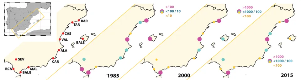
In our case, the compositional approach allows to study the evolution of the container throughput from a relative perspective. In this work, we have selected the Spanish ports located in the Mediterranean range (SpanishMed). This area includes 11 ports. The location of these ports is shown in Fig. 1. The SpanishMed area covers a rele-vant market in the European context and includes two
of the top ten European ports in container throughput: Valencia and Bahía de Algeciras. The hinterland of this region extends to a high portion of Spain and South of France, competing with Portuguese and North African ports to capture container transshipment activity.
The objective of this paper is double. As a first stage it aims to introduce the CoDa formalism and highlight its potentiality in the port container throughput analysis as example of transport system providing an applied exam-ple: SpanishMed ports. Second, based on the previous analysis, the aim is to characterize the container through-put in SpanishMed ports and its temporal evolution.
The contribution is organized as follows: a short description of the container throughput evolution of the SpanishMed ports is presented (Section 2). Then, the CoDa methodology is briefly introduced (Section3). The results from the CoDa exploratory tools are shown in Sections4and5for a sub-sample and for the whole system respectively. In Section6results are discussed, remarking the insight provided by CoDa techniques in the Span-ishMed ports analysis as example of research in transport discipline.
2 SpanishMed port system
The state-owned Spanish Port System includes 46 ports of general interest, managed by 28 Port Authorities, whose coordination and efficiency control corresponds to the Spanish Port Agency (Puertos del Estado;www.puertos.es), a body seconded by the Ministry of Public Works that is responsible for implementing the government’s port
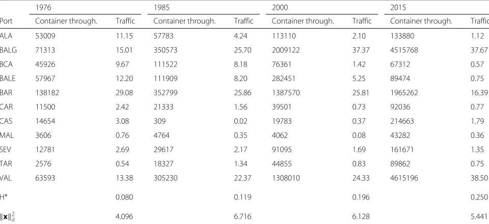
policy. SpanishMed ports include 11 Port Authorities (see Fig. 1). The data were obtained from the Spanish Port Agency (integrated annual data). Small ports, some of them owned by regional governments, are excluded from this analysis because their container throughput is negligible. The total container throughput in Span-ishMed arose 11.988.405 TEU (Twenty-foot Equivalent Unit) during 2015. The main ports are Algeciras Bay, Valencia and Barcelona covering a traffic share of 37.67%, 16.39% and 38.50% respectively during 2015 (see Table1). A preliminary analysis indicates that port throughput concentration occurs according to the traffic evolution for the period 1976–2015 according to the normalized Herfindahl-Hirschman index [24] shown in Table1. More than 90% of the traffic during 2015 corresponds to these three ports, with also large percentages for 2000, 1985 and 1976 (87.5%, 73.9% and 57.5% respectively).
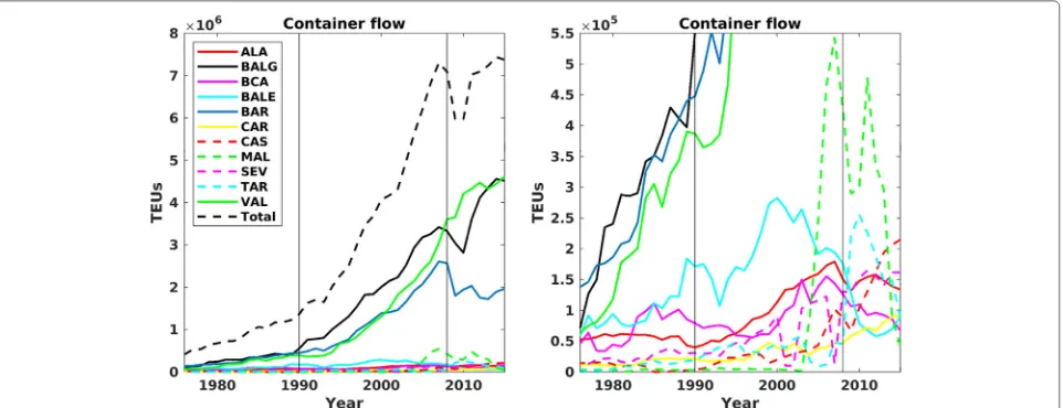
The temporal evolution of the Spanish Med container throughput is shown in Fig.2in terms of total traffic evo-lution. The container flow at SpanishMed has a container-ization peak growth (1995–2010) followed by a maturity phase (2010-today). This suits well in a K-wave behav-ior which specific phases in container port development are taking place, such as introduction, acceleration, peak growth and maturity [18]. Considering only the “three-big” ports, the evolution of the traffic share at the Span-ishMed system shows a gentle decreasing of the Barcelona and Algeciras Bay port traffic as opposite to an increase of Valencia Port after 2007 (crisis period). Among other motivations this behaviour is due to the 2002 selection of
Table 1Total number of containers (in TEU) and traffic share (in %) for the SpanishMed ports during years 1976, 1985, 2000 and 2015
1976 1985 2000 2015
Port Container through. Traffic Container through. Traffic Container through. Traffic Container through. Traffic
ALA 53009 11.15 57783 4.24 113110 2.10 133880 1.12
BALG 71313 15.01 350573 25.70 2009122 37.37 4515768 37.67
BCA 45926 9.67 111522 8.18 76361 1.42 67312 0.57
BALE 57967 12.20 111909 8.20 282451 5.25 89474 0.75
BAR 138182 29.08 352799 25.86 1387570 25.81 1965262 16.39
CAR 11500 2.42 21333 1.56 39501 0.73 92036 0.77
CAS 14654 3.08 309 0.02 19783 0.37 214663 1.79
MAL 3606 0.76 4764 0.35 4062 0.08 43282 0.36
SEV 12781 2.69 29617 2.17 91095 1.69 161671 1.35
TAR 2576 0.54 18327 1.34 44855 0.83 89862 0.75
VAL 63593 13.38 305230 22.37 1308010 24.33 4615196 38.50
H∗ 0.080 0.119 0.196 0.250
x2
a 4.096 6.716 6.128 5.441
Ports are identified as follows: ALA (Alacant/Alicante), BALG (Bahía de Algeciras or Algeciras Bay), BCA (Cádiz Bay), BALE (Balearic Islands), BAR (Barcelona), CAR (Cartagena), CAS (Castelló/Castellón), MAL (Málaga), SEV (Sevilla), TAR (Tarragona), VAL (Valencia). The values of the normalized Herfindahl-Hirschman index (H∗) and squared Aitchison normx2
a
Grifollet al. European Transport Research Review (2019) 11:12 Page 4 of 15
Fig. 2(left) Evolution of the total container throughput at SpanishMed ports. (right) Zoom of the lower range of the total container throughput. The three biggest ports are BALG (black line), BAR (blue line) and VAL (green line). Reference lines for years 1990 and 2008
Valencia as the hub port for MSC shipping company and the good response of the transshipment flow in Valencia after the crisis. The Barcelona container traffic was hit hard by the crisis with a significant decrease of container flow (from 2.6 million TEUs during 2008 to 1.8 million TEUs in 2009). Actually an equal percentage of traffic share occurs between Valencia and Algeciras Bay (both of them with relevant percentage of transshipment flows) followed from a certain distance by the Barcelona port, which its traffic is mainly focused on the import/export activity.
3 The CoDa methodology
Compositional Data (CoDa) are defined as a quantitative description of the parts of a whole [28]. In fact, a compo-sition is a class of equivalence, i.e., proportional vectors provide the same compositional information. Usually, a representative of the class of equivalence is chosen. The suitable sample space for the representation of composi-tional vectors is the SimplexSD(Eq.1):
SD=
x=[x1,x2, ...xn] :x1>0,x2>0,. . .,xn>0; D
i=1
xi=c
.
(1)
A composition x =[x1,. . .,xD] is defined as a vector
withDstrictly positive components adding to a constant (c), where the constantcis the closure. The closure is the vector operation assigning the constant sum representa-tive of the composition. Frequently,cis 100 for measure-ments represented in percentages. The simplex is charac-terized as a vector space using two operations: perturba-tion and powering [28]. The so-called Aitchison geometry for the simplex also includes a distance. The Aitchison
distance between two compositionsx=[x1,. . .,xD],y =
[y1,. . .,yD] is defined as (Eq.2):
da(x,y)= 1
2D D
i=1 D
j=1
ln
xi xj
−ln
yi yj
2
, (2)
and the corresponding norm is (Eq.3):
xa= 1
2D D
i=1
D
j=1
lnxi
xj 2
. (3)
The principles of compositional analysis include three conditions that should be fulfilled by the statistical meth-ods that are applied to compositions: scale invariance, permutation invariance, and subcompositional coherence [2,28]. In subsequent sections we will take advantage of the subcompositional coherence property for the treat-ment of the container throughput in the SpanishMed port system.
Given a sample of size n of D-part compositional vectors, X, [x11,. . .,x1D] ,. . .[xn1,. . .,xnD], it is usual
to describe them using central tendency and variability measures. The standard statistical descriptive measures, based on the real Euclidean structure, applied to Compo-sitional Data may lead to erroneous conclusions. An alter-native set of descriptive measures, based in the Aitchison geometry has been defined. The center (cen), Eq.4, is a measure of central tendency of the compositional sample:
cen(X)=[g1,. . .,gD] , (4)
beinggithe column-wise geometric mean:
gj(x)= n
i=1 xij
1/n
The definition of the concept of distance between two compositions (Eq.2) is relevant for the statistical analysis of compositional data because it allows to define basic sta-tistical concepts such as variability. The variation matrix is a measure of the data dispersion and it is defined in terms of pairwise log-ratio variances (Eq.6) [2,28]:
T= ⎛ ⎜ ⎜ ⎜ ⎝
0 t12 . . . t1D t21 0 . . . t2D
..
. ... . .. ...
tD1 tD2 . . . 0
⎞ ⎟ ⎟ ⎟
⎠,tij=var
lnxi
xj
. (6)
The sample total variance (Eq.7) is a measure of global dispersion of the compositional sample, being a summary of the variation matrix in a single quantity.
totvar(X)= 1
2D D
i,j=1
var
lnxi
xj = 1 2D D
i,j=1
tij. (7)
Also, Aitchison norm (Eq.3) may provide an estimation of the concentration level of container throughput ports similar to Herfindahl-Hirschman index.
The mathematical structure of the Simplex as an Euclidean vector space gives the possibility of treating compositional data in a suitable manner. However, the fact that the information given by compositions is rela-tive was the origin of the so-called principle of working in coordinates [2, 21]. That is, transforming composi-tions into real vectors, for which the usual real Euclidean structure is suitable. Several transformations based on log-ratios have been defined in the literature [2,13]. His-torically, the additive log-ratio (alr) was the first to be used and the centered-log ratio (clr) appeared later; both introduced by [1,2]. The third family of transformations is theilr(isometric log-ratio transformation) which pro-vides Cartesian orthonormal coordinates [13]. The clr transformation of a compositionx=[x1,. . .,xD] is:
clr(x)=ln
x1
gm(x)
, x2
gm(x)
, x3
gm(x)
,. . ., xD
gm(x)
, (8)
where gm(x) denotes the geometric mean of the parts
(Eq.9).
gi(x)= D
i=1 xi
1/D
. (9)
The mentioned transformations (alr/clr/ilr) have dif-ferent properties. The alr transformation has the incon-venience that the transformation is not isometric, i.e. it does not preserve distances. This implies that the use of the inner-product or the determination of the angle between two vectors became more difficult [11]. The clr-transformation keeps the same number of components
as the number of parts in the composition: a sition with D parts is transformed into D real compo-nents adding up to 0 [13]. This transformation preserves the metrics (i.e. the distances and the angles). That is, the distance between two compositions measured in the Simplex using the Aitchison distance (Eq.2) and the dis-tance between their transformed vectors using the usual real Euclidian distance are the same. Therefore, the clr-transformation may be useful as exploratory tools based on metrics, such as the biplot. However, the clr-transformation has the inconvenience that the covariance and correlation matrix are singular (i.e their determinant is zero), due to the zero-sum of the transformed vectors.
The isometric log-ratio transformation (ilr) [13] appears as an alternative when statistical tools based on covariances are needed. Compositions are expressed as coordinates with respect to an orthonormal basis. This transformation corresponds to an isometry of vector spaces between the simplex ofD-partsSD(Eq. 1) and
RD−1. In order to enhance interpretability, an
orthonor-mal basis linked to a Sequential Binary Partition (SBP) is often selected [28]. The SBP is encoded through a sign matrix, that allows the practitioner to define a hierarchy of the parts of the composition based on knowledge about the problem at hand. The coordinates obtained in such manner are called balances, and they are the normalized log-ratios of the geometric mean of the groups of parts defined by the sign matrix at each step. Balances have the form (Eq.10):
bj=
rs r+sln
gm(x+) gm(x−)
. (10)
wherer andsare the number of parts in the+1-group and−1-group respectively.
4 Subcompositional analysis of SpanishMed: BALG, BAR and VAL.
In order to introduce the compositional methodology in the SpanishMed system, this section focuses only in the subcomposition formed by the three biggest ports: Algeci-ras Bay (BALG), Barcelona (BAR) and Valencia (VAL; see all acronyms in Fig.1). The subcompositional coherence property ensured by the compositional approach guaran-tees that the results obtained for this subsample will be coherent with the results obtained for the whole system. As we mention previously, these three ports have reached 90% of the traffic share in SpanishMed in the recent years (see Fig. 2 and Table1). Figure2 shows the raw traffic evolution for the SpanishMed system where these three ports show a relevant role in the traffic share. There is an increasing trend in traffic, although there are some ups and downs since 2008.
Grifollet al. European Transport Research Review (2019) 11:12 Page 6 of 15
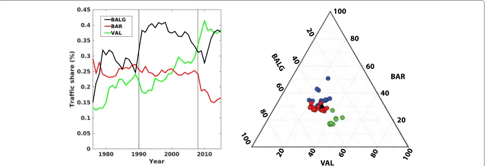
Fig. 3(left) Traffic share evolution of the three biggest ports (%). (right) Ternary diagram of the BALG/BAR/VAL traffic composition. Blue dots correspond to the period 1976–1989 (before containerization boom), red dots correspond to the period 1990–2007 (before the crisis) and green dots correspond to the period 2008–2015. The center of the sample is shown as a black triangle
contribution of each port has a different interpretation in comparison to the total traffic (Fig.2). It means, two of the ports increase their share (BALG and VAL), whilst the third one (BAR) loses relative importance. From a temporal point of view, this may be linked to three main events: the boom of the containerization in the 1990s, the selection of VAL Port as a basis for shipping com-pany MSC in 2002 (and its posterior development as a transshipment hub) and the 2008 crisis. The crisis effects implied a decrease of the total container throughput (see Fig. 2). These change points in the traffic evolution are also observed if the traffic share is represented using a ternary plot (Fig.3). The ternary plot is a barycentric plot which graphically depicts the ratios of the three variables as positions in an equilateral triangle. The figure shows the temporal evolution of the compositions of the traffic share considering the containerization boom in 1990 and the post-crisis (see blue, red and green colored points). The evolution of the cloud of points shows a predominance of BAR during the initial years (before containerization; blue points), the prevalence of BALG port after the container-ization (red points) and the leadership in traffic share of VAL port after the crisis/MSC settling effect (green points).
The center of this cloud of points (i.e. the center of the sample of compositions, Eq.4, marked with a black triangle) is near to the baricenter of the triangle, with a slight shift due to the influence of BALG port. The sample center value is shown in Table2. From a historical point of view the center reveals a predominance of the BALG port with a more than 40.2% of the traffic share. Table2also shows the variability of the composition (variation array in Eq.6). The maximum variability is associated to BAR port (e.g. variances equal to 0.146 and 0.216) due to the traffic fluctuations caused by the 2008 crisis.
The principal components for compositional data were introduced by [5]. The biplots for compositional data (clr-biplots) were introduced by [4] and they have been a powerful tool for multivariate analysis [10,28]. The clr-biplot is an exploratory tool that allows to display data and variables in the same plot. The dimensionality of the dataset is reduced, as the original information is repre-sented in a projection on two new variables. A principal component analysis of the clr-transformed compositions is performed. The clr-biplot corresponds to the projec-tion of the informaprojec-tion of the dataset in the 2-dimensional plane formed by the two first components. The visual interpretation of clr-biplots differs slightly from that of the general biplots. Form and covariance clr-biplots highlight different characteristics of the data in the projection. The form clr-biplot helps with the assessment of the goodness of the representation of the variables in the projection. The covariance clr-biplot helps with the assessment of the variability and relationships between the variables. The principal elements of interpretation of clr-biplots are the rays and the links formed by the rays. Some rules were highlighted by [10]. For instance, if three rays are aligned, then the relation between these parts is linear up to the quality of the projection. Also, orthogonal links mean that two sub-compositions are uncorrelated. The covariance
Table 2Variation array of the traffic throughput yearly composition
Port BALG BAR VAL cen(x) (%)
BALG 0.000 0.146 0.103 40.2
BAR 0.146 0.000 0.216 30.0
VAL 0.103 0.216 0.000 29.8
clr-biplot includes specific information of the variability through the length of the rays.
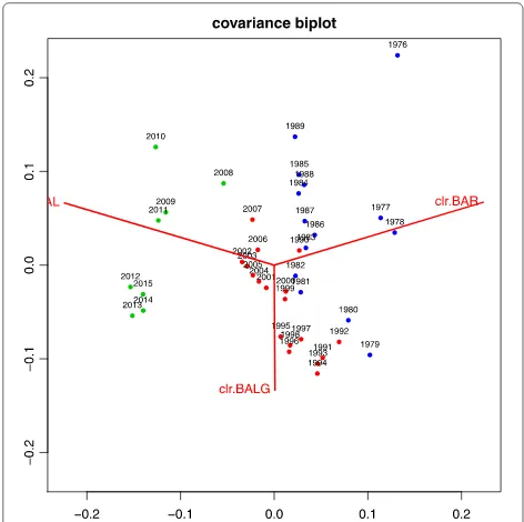
The covariance clr-biplot of the three big ports (BALG-BAR-VAL) is presented in Fig.4. The shown projection represents 100% of the variance and the three variables are exactly represented in the form clr-biplot, so it is omitted for simplicity. The longitude of the rays in the covari-ance biplot (Fig. 4) is proportional to the variability of the clr-variable. BALG is slightly less variable than VAL and BAR ports. This reflects the aforementioned traffic variation array of Table2, where the maximum pairwise variance is between BAR and VAL. The position of the yearly compositions in the graph suggests a temporal evo-lution. In the initial years, the points are near to BAR ray, then shifting towards BALG ray in the first waves of containerization (red points). Since the 2000’s there is an evolution towards VAL ray (green points). This increase is more moderate since the start of the crisis; but the influ-ence of the pair VAL – BALG is reinforced in contrast to BAR. Figure2highlights the change points defined before: the boom of the containerization that attracted traffic to BALG and the combined effect of the MSC settling in VAL and the crisis attracting traffic to VAL. After the cri-sis the evolution is clear: VAL maintains its influence, but BALG recovers part of the lost traffic (green points). As only three variables are represented, this interpretation is similar to that obtained for the ternary diagram (Fig.3).
Fig. 4Covariance Biplot. BALG-BAR-VAL traffic composition. The projection represents 100% of variance. The longitude of the rays is proportional to the variability of the clr.variable. Blue dots corresponds to the period 1976–1989 (before containerization boom), red dots correspond to the period 1990–2007 (before the crisis) and green dots correspond to the period 2008–2015
The cosinus of the angle between two links of the rays is an approximation to the linear correlation coefficient between the corresponding simple log-ratios. The links between the rays of clr(VAL) and clr(BALG)-clr(BAR)) are nearly orthogonal, suggesting a low correla-tion between these ratios. In fact, the correlacorrela-tion between ln(BALG/BAR) and ln(BALG/VAL) is -0.110. The cor-relation between ln(BAR/BALG) and ln(BAR/VAL) is 0.744, and finally ln(VAL/BALG) and ln(VAL/BAR) is 0.747. These values confirm the relative dependence of BAR with the others ports. In opposite, BALG has a more differentiated behaviour. In any case, the obtained values of correlation between the log-ratios is consistent with the previous analyses of the rays.
In order to deepen the interpretation of the evolution of the traffic composition, an ilr transform of the compo-nents has been also performed. The selected sequential binary partition (SBP) corresponds to Table3. From the selected SBP, two balances are built:
b1=
2 3ln
BALG √
BAR·VAL
; b2=
1 2
BAR VAL
,
(11)
where the first balance accounts for the logratio between BALG port and the geometric mean of the other two ports, and the second balance is the logratio of BAR port versus VAL port.
The codadendrogram (Fig. 5) is an useful exploratory tool that helps with the description of these balances. This graphical representation also shows the ilr decomposition of the total variance, as well as the mean and dispersion of each balance. The length of the blue vertical bars shown in Fig. 5 is proportional to the variance of the balance [14, 27]. In this case, the second balance, BAR vs. VAL, has a higher variance than the first one (BALG vs the geo-metric mean of BAR and VAL). The point where these verticals bars join the horizontal bars is the mean balance, i.e. the coordinate corresponding to the sample center (Eq.4). For both balances this point is close to the mid-dle of the horizontal bar. This is consistent with the mean of the balances that are 0.243 and 0.003 for each balance. The figure also shows a characterization of the ilr dis-persion through a box-plot of the corresponding balance, where balance ranges and quartiles are also presented (see example in [28]). In the figure, the box-plot of the first bal-ance shows some asymmetry and more dispersion than the box-plot of the second balance.
Table 3Sequential Binary Partition for the three big ports
Balance BALG BAR VAL
b1 1 -1 -1
Grifollet al. European Transport Research Review (2019) 11:12 Page 8 of 15
Fig. 5Codadendrogram. Balances of BALG-BAR-VAL traffic composition following the selected SBP (Table3)
The addition of a factor variable to the codadendrogram may be also useful. Figure6 shows the codadendrogram corresponding to the selected SBP, adding a time-evolution factor: the initial years (blue lines), the con-tainerization boom period (red lines) and the post-crisis years (green lines). The figure shows some changes in the balances. The vertical bars corresponding to the ini-tial years of the balances show a higher variance than the bars corresponding to the next years. This is due to the fluctuations of the traffic share evolution without any
clear leadership in comparison to the subsequent periods (see Figures2and3). The boom of containerization was marked by a leadership of the BALG in its traffic share, which meant small fluctuations in the traffic share evolu-tion. This is reflected by the low coordinate variances (red vertical bars) in Fig.6. Afterwards, the variance of the bal-ances of the post crisis years increased, due to the different adaptation of the ports after the 2008 crisis. In this sense, the three ports behave very differently: VAL increases sig-nificantly its traffic due to the role that played the settling
of MSC base in 2002, BALG maintains its relevance after post-crisis fluctuations in its traffic share and BAR loses its influence in the sub-composition. The center of the first balance changes only slightly for the three periods. In opposite, the changes are significant for the second bal-ance (VAL vs BAR), showing an increasing influence of the VAL port.
5 SpanishMed container throughput: a compositional data (CoDa) approach
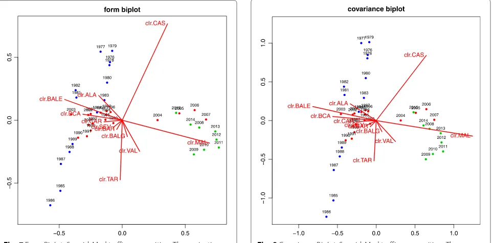
Once the sub-composition of the three main ports has been analysed using CoDa, all the SpanishMed ports are considered. Figure2 shows the total container through-put and the correspondent traffic share evolution. Figure2 (right) shows a zoom of the total traffic to highlight the temporal evolution of the smaller ports. Figure 7shows the form clr-biplot for the container throughput com-position of the SpanishMed ports. It corresponds to the projection on the two first components and accounts for 68% of the total variability. The three first components account for 86% of the variance. The low alignment pat-tern of the rays (spreading of the variables in the form clr-biplot) also indicates the relative low explanation of the new projection axis. The form clr-biplot helps with the assessment of which variables are better represented in the projection. Ideally, if all the variables were well rep-resented in the projection, the rays would have the same length. In the Fig.7, CAS(Castelló), MAL (Malaga) and BALE (Balearic Islands) ports are the ones with a better
Fig. 7Form Biplot. SpanishMed traffic composition. The projection represents more than 68% of variance. Blue dots correspond to the period 1976–1989 (before containerization boom), red dots correspond to the period 1990–2007 (before the crisis) and green dots correspond to the period 2008–2015
representation on this projection. Also, these ports are the ones with more variability, following the covariance biplot (Fig.8). These three ports (BALE, CAS and MAL) show large rays; this is due to its small container volume imply-ing that their relative changes are larger meanimply-ing more volatility. For instance, MAL port had a large volatility in its traffic share being relevant during 2012 (4.7%) as opposed to years 1985, 2000 or 2015 (see Table1). CAS is characterized by a gentle increase of the traffic share after 2000 being the fourth port in importance in total throughput and traffic share during 2015. This pattern is not followed by other ports and therefore CAS port appears isolated in the first quadrant of the projection. Also, a high volatility in the traffic share is observed in BALE, which shifted from 8.20 to 0.75% of the traffic from 1985 to 2015 (note that this evolution is clearly different to the MAL case, consistently with the interpretation of the clr-biplot). The other ports are not represented so well in this projection, probably due to their smaller variability.
Some ports (e.g. ALA (Alacant), BALE, BCA (Cádiz Bay)) show a nearby location in the projection on the covariance clr-biplot. This set of ports has a similar pat-tern of variability, in particular a gentle decreasing of traffic share from 1985 to 2015 (see Table1). According to the covariance clr-biplot, also a similar pattern is observed for the set of ports formed by SEV (Sevilla), BAR and CAR (Cartagena). According to Table 1 this behavior is associated with a relative loss of traffic share in 2015 in comparison to 1985. The alignment of the rays of BALG,
Grifollet al. European Transport Research Review (2019) 11:12 Page 10 of 15
BAR and VAL (the three big ports) also indicates that the three ports do no have a very different pattern in compari-son to other ports. Figures7and8also shows the temporal evolution of the CAS port traffic share. During the eighties this port lost importance, recovered during the nineties. The evolution since 2004 is toward a composition where the MAL port gains importance, but the figure also shows the evolution of the parts of the three more important ports (BAR-BALG-VAL). These three ports are not very well represented in the projection, and are characterized by a small variability until 2012, when its importance started to decrease. These figures also show that since 2004 the SpanishMed traffic composition evolves from a BAR influence area to a VAL influence area, consis-tent with the findings in Section4and agreeing with the sub-compositional coherence principle [28].
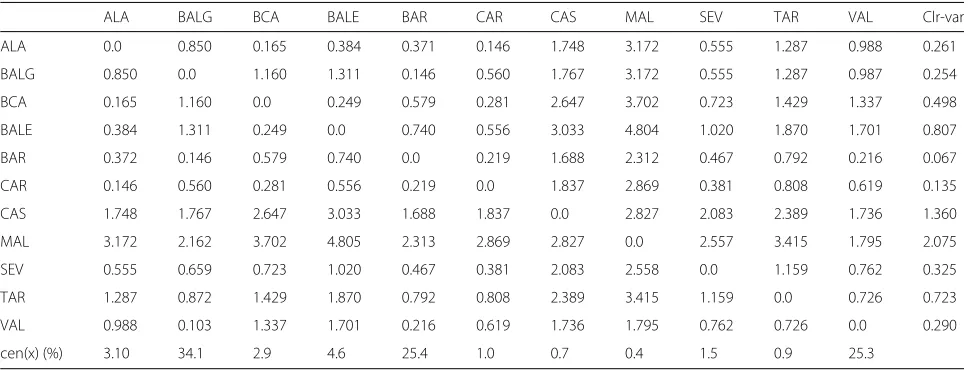
The relationship between clr-variables may be also assessed through the covariance clr-biplot. In the figure, the links between the rays clr(BALE)-clr(CAS) and clr(CAS)-clr(MAL) are nearly orthogonal and there-fore the corresponding simple log-ratios present low correlation. When computed, the corresponding lin-ear correlation coefficient between ln(BALE/CAS) and ln(CAS/MAL) is -0.18. The orthogonality of links is clearer for the clr(BALE)-clr(MAL) and clr(VAL)-clr (CAS). The linear correlation coefficient corresponding to their log-ratios, ln(BALE/MAL) and ln(VAL/CAS) is 0.05. An additional assessment of the relationships between pairs of ports is provided by the variation matrix (Table 4). In this case, substantial log-ratio nor-malized variances agree with the clr-biplots interpretation (i.e. clr(BALE)-clr(CAS) equals to 3.033 and clr(MAL)-clr(CAS) equals to 2.827. The smallest contributions are the ones between the clr(BAR) and clr(BALG) variances (0.146), followed by the contributions which relate ports
such as ALA, SEV or VAL (see clr-variances in Table4). This confirms the assessment provided by the covari-ance clr-biplot, where the rays corresponding to these ports are proportional (showing a similar pattern) and the contribution to variability is redundant. The largest con-tribution to variability is provided by MAL (clr-variances equals to 2.075) and CAS (clr-variances equals to 1.360) consistent again with the assessment of the clr-biplot: there is a low correlation of both variables with the other ports.
For further assessment of the SpanishMed traffic com-position, an ilr transformation has also been performed. The selected SBP is shown in Table5. The corresponding balances compare ports with different characteristics. For instance,
b1=
10 11ln
BALE g(rest)
; b4=
1 2ln
BAR VAL
,
(12)
b2=
21 10ln
(
BALG·BAR·VAL)1/3
g(remaining 7 ports)
.
Some of the criteria used to build the balances are described as follows. Balance b1corresponds to the
bal-ance of BALE port with the geometric mean of the rest of the ports. The insular nature of this port suggests a low dependence with the others and consequently a high vari-ability of the balance. The second balanceb2corresponds
to the comparison of the geometric mean of the three big ports with the geometric mean of the non-insular ports of the system. Due to the subcompositional coherence of the compositional treatment of the shares,b3andb4
coin-cide with Eq. 11, that is, the balances that compare the sub-system of the three big ports.
Table 4Log-ratio normalized variances of the traffic throughput yearly compositions
ALA BALG BCA BALE BAR CAR CAS MAL SEV TAR VAL Clr-var
ALA 0.0 0.850 0.165 0.384 0.371 0.146 1.748 3.172 0.555 1.287 0.988 0.261
BALG 0.850 0.0 1.160 1.311 0.146 0.560 1.767 3.172 0.555 1.287 0.987 0.254
BCA 0.165 1.160 0.0 0.249 0.579 0.281 2.647 3.702 0.723 1.429 1.337 0.498
BALE 0.384 1.311 0.249 0.0 0.740 0.556 3.033 4.804 1.020 1.870 1.701 0.807
BAR 0.372 0.146 0.579 0.740 0.0 0.219 1.688 2.312 0.467 0.792 0.216 0.067
CAR 0.146 0.560 0.281 0.556 0.219 0.0 1.837 2.869 0.381 0.808 0.619 0.135
CAS 1.748 1.767 2.647 3.033 1.688 1.837 0.0 2.827 2.083 2.389 1.736 1.360
MAL 3.172 2.162 3.702 4.805 2.313 2.869 2.827 0.0 2.557 3.415 1.795 2.075
SEV 0.555 0.659 0.723 1.020 0.467 0.381 2.083 2.558 0.0 1.159 0.762 0.325
TAR 1.287 0.872 1.429 1.870 0.792 0.808 2.389 3.415 1.159 0.0 0.726 0.723
VAL 0.988 0.103 1.337 1.701 0.216 0.619 1.736 1.795 0.762 0.726 0.0 0.290
cen(x) (%) 3.10 34.1 2.9 4.6 25.4 1.0 0.7 0.4 1.5 0.9 25.3
Table 5Sequential Binary Partition for the SpanishMed port system
Balance ALA BALG BCA BALE BAR CAR CAS MAL SEV TAR VAL
b1 -1 -1 -1 1 -1 -1 -1 -1 -1 -1 -1
b2 -1 1 -1 0 1 -1 -1 -1 -1 -1 1
b3 0 1 0 0 -1 0 0 0 0 0 -1
b4 0 0 0 0 1 0 0 0 0 0 -1
b5 -1 0 -1 0 0 -1 -1 1 -1 -1 0
b6 -1 0 -1 0 0 -1 1 0 -1 -1 0
b7 -1 0 -1 0 0 -1 0 0 -1 1 0
b8 -1 0 -1 0 0 1 0 0 -1 0 0
b9 1 0 -1 0 0 0 0 0 -1 0 0
b10 0 0 1 0 0 0 0 0 -1 0 0
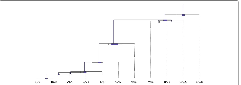
The codadendrogram of the SpanishMed ports bal-ances, following the selected SBP (Table 5), is shown in Fig. 9. The vertical bars, proportional to the vari-ances of the balvari-ances, show very different lengths. The longer bar corresponds to the fifth balance, that is the balance of the MAL port with respect to the geomet-ric mean of the remaining ports. The second longer bar corresponds to the balance of CAS port with the geomet-ric mean of the remaining ports (b6). The fifth balance
(Eq.12) also shows a mean balance that is clearly far from zero. This means that this balance (associated to MAL port) has relevant fluctuations during the analysed period. These interpretations are consistent with the con-clusions drawn from Fig.7 in regard to MAL and CAS ports. For other balances, for instance for the last bal-ance (SEV vs BCA), the mean is likely zero. The box-plots show also different ilr variability patterns. For instance, the second balance shows a large ilr-dispersion, with some
asymmetry. This is related to the specific characteristics of the traffic share evolution of MAL port, previously explained. Other balances, for instance the VAL-BAR bal-ance, show not only more ilr-symmetry, but also less ilr variability.
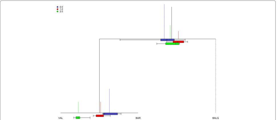
The introduction of the temporal evolution factor to the codadendrogram shows changes in the variances of the balances (Fig.10). During the initial years, the variance of the market (blue vertical lines) is large in comparison to the subsequent periods. This is due to the small differ-ences among the traffic share evolution in comparison to the boom of containerization when three ports rule the market. It means, the evolution in a concentrated market (seeH∗in Table1) implies larger variability. For some of the balances, the evolution of the mean balance is clearly observed. For instance, the balance CAS vs the geomet-ric mean of the remaining ports shows an evolution of the mean balance towards CAS, i.e. the proportion of traf-fic share of CAS port respect the geometric mean of the remaining ports is higher after the crisis than in the early years (see Fig.2). This is consistent with the interpreta-tion of the clr-biplot (Fig.8) and the traffic share evolution shown in Table1.
As mentioned in Section 3, one of the principles of compositional analysis is subcompositional coherence. In our case, this condition means that the statistical results obtained through the analysis of the whole Spanish port system and the analysis of the subsample formed by BALG, BAR and VAL are coherent. In fact, the selected SBPs lead to the same results. For instance, the balanceb2
for the subcomposition (see Table3) and the balanceb4
for the total SpansihMed analysis are the same. These bal-ances correspond to the ratio BAR vs. VAL. The analysis of the balance from both points of view (Figs.6 and10) shows a temporal evolution with a shift of the center of the balance towards VAL port.
Grifollet al. European Transport Research Review (2019) 11:12 Page 12 of 15
Fig. 10Codadendrogram. SpanishMed balances of traffic composition following the selected SBP ((Table5). Color: Blue corresponds to the period 1976–1989 (before containerization boom), red corresponds to the period 1990–2007 (before the crisis) and green corresponds to the period 2008–2015. The yellow box show a zoom of the BALG-BAR-VAL balances that is coherent with Fig.6
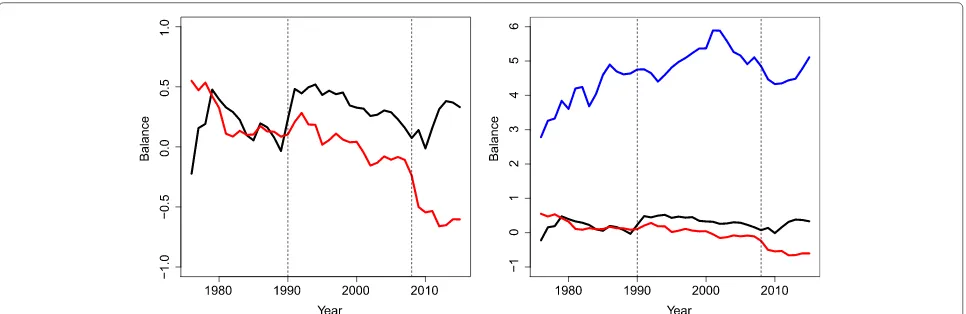
The temporal evolution of the balances also suggests an interpretation of the temporal evolution of the traf-fic share among the ports. Figure11shows the balances time-series for the three big ports:b1andb2. The balance
b1shows a significant temporal variability without a clear
trend during the analysed period. In opposite, theb2
bal-ance shows a negative slope which means that BAR port loses traffic share in front of VAL (see Eq.11). Figure11 also shows the b2 balance time-series (the three main
ports vs the non-insular ports) when all the SpanishMed container system is investigated. The time-series shows how the big-ports gain importance in front of the small ports until 2002. Then a fluctuation period occurs before and after the crisis.
6 Discussion
In the framework of the ocean container transport and shipping, CoDa techniques help with the interpretation of the dependencies in the growths of traffic shares. The description of the evolution of the traffic share is not simple. Ocean container traffic is a complex and multi-faceted system where shippers, logistic services providers and shipping lines do not necessarily choose a port or port system, but they select a chain in which a port is merely a node [25]. From a historical point of view there is an increase of the traffic growth responding to the boom of the containerization jointly with the emergence of the global transport networks [18]. However, not all ports respond in the same way: the evolution of the SpanishMed
Fig. 11(left) Evolution of the balances corresponding to the three big ports following the selected SBP (Eq.11). First balanceb1(black line); second
balanceb2(red line). (right) Evolution of three selected balances of the SpanishMed ports following the selected SBP (Table5). The blue line shows
the evolution of the balance that compares the three big ports with the rest of the non-insular ports (b2; Eq.10). Black and red lines represent the
balances between the three big ports, according to the selected SBP (b3andb4). Note that the compositional treatment of the shares ensures
ports has evidenced a gradual increase in the concen-tration of activities in only a few ports (see Herfindahl-Hirschman index and Aitchison norm in Table 1). The need to implement economies of scales has led to two dif-ferent port orientations in function of the market: large load centres or hubs (oriented to receive deep sea inter-continental ships) and smaller regional or feeder ports (with a prevalent percentage of import/export or feeder activity). Bahía de Algeciras (BALG) and Valencia (VAL) are examples of the former and Barcelona (BAR) an exam-ple of the latter. The inclusion of CoDa techniques has allowed to confirm this tendency from an analytic point of view. In particular, the data association and dependen-cies obtained by the clr-biplot evidences the connection between BAR and the other ports. Barcelona lost traffic share (due to a decrease of transshipment flows) in favor to the hubs of VAL and BALG as a result of the com-petition dynamics. This conclusion is not only obtained through the clr-biplot assessment, also the ternary plot interpretation and the computation of the linear corre-lation between the log-ratios agree to this point. This example illustrates the potentiality of CoDa methods in the traffic share description in a transport system being consistent with other authors (e.g. [24] or [9]).
The difference of magnitudes of the container through-put among different ports (for instance the container throughput in VAL port is 100 times larger than for Málaga (MAL) port) evidences the potentially of the CoDa methodology where the interest lies in the relative mag-nitude and variations within the system instead of the absolute values. It is worth mentioning the ability of CoDa analysis to investigate the patterns of evolution of small ports. Their behaviour may be hidden using conventional techniques. This is the case of CAS port, which traf-fic share evolution is uncorrelated with the other ports. CAS port has been able to capture and consolidate an alternative in the container throughput market in the SpanishMed system. In this sense, BALE and MAL ports also show a differentiated pattern. The rest of the ports reveal a similar pattern of variability in comparison to the mentioned ones. In consequence, relationships and simi-larity patterns have been detected. The loss of importance of the Barcelona (BAR) port has also been noted in the analysis of the results, where the turnover point of the total container throughput during 2008 has been pointed out. The global economic crisis during 2008 or the excep-tional development of Valencia port in terms of container throughput have also been detected using CoDa descrip-tive tools. The assessment of the temporal evolution of the balances has allowed to investigate the response of the ports against the crisis among other interesting features. For instance, the balance b3 time-series (Fig. 11) shows
how the traffic share of the big ports is maximum during 2002 after a gentle increase. The subsequent decrease of
the contribution of the big ports may be associated with the “challenge of the periphery” [24] where new incom-ers appear with substantial traffic share (for instance CAS port) due to the congestion of existing big ports or the increase of the connectivity of the smallest ones. This tendency is also maintained during period 2008–2010, where it seems that the smallest ports experienced better resilience to the crisis. Finally, the three big ports recover importance during the period 2013–2015 probably due to the traffic retrieval in BAR port. Since the examined ports is a state-owned system, the investigation may have policy implications related to port categorization, competitive evaluation or resource assignment based on traffic share evolution.
The benefit of CoDa techniques to investigate trans-port disciplines is clear. Standard statistical techniques, based on the real Euclidean space, may provide mis-leading information about relations or similarity of the temporal evolution port traffic share. Temporal evolution of the market concentration/deconcentration is a typi-cal approach to identify the variability of the traffic in a system. For instance, this analysis has been carried out on airports and air-flight companies (e.g. [30] or [26]) using concentration indexes (Herfindahl-Hirschman or Gini coefficients). This kind of analysis may reveal oppor-tunities and threats for future investments in various types of transport infrastructure [30]. In SpanishMed, the inclu-sion of CoDa techniques has complemented the interpre-tation ofH∗evolution and the Aitchison distance with its link with the variability of the market in the early years. Other areas of transportation engineering such as modal competiton or service complementarity may be benefited from using the CoDa approach. Other research works applying CoDa on socio-economic problems, such as [31] or [28], have revealed promising results identifying partic-ular patterns on data as uneven as nutrition, social science or production engineering.
Grifollet al. European Transport Research Review (2019) 11:12 Page 14 of 15
ANOVA to the mean balances to assess if the differences are significant in the selected temporal periods. In the framework of port systems, the introduction of the CoDa techniques to the transshipment market may be useful. This market tends to be more unstable and volatile [25], so the inclusion of other kind of external variables [12] may be used in order to get insight into the market evolution.
7 Conclusions
The SpanishMed port system has been used as an exam-ple of introducing the CoDa methodology in transport disciplines. However, this is a wide applicable methodol-ogy, that should be applied to other geographical regions and other fields to understand the spatial integration that results in the movement of people and freight. The methodology has allowed to establish port associations, underlying patterns and to investigate tendencies avoiding spurious correlations that arise from the use of conven-tional statistical techniques. The original findings in the SpanishMed system analysis using CoDa is the emerg-ing of small ports with a differentiated pattern (challenge of the periphery), the connection of the traffic share of Barcelona port with Valencia and Algeciras Bay ports (port competition) and the concentration process in the mentioned 3-big ports. The examined data and the practi-cal conclusions may have relevant implications for policy makers due to the state ownership of the investigated port system.
Acknowledgements
The authors acknowledge Spanish Ports Agency (Puertos del Estado) for the port traffic data provided.
Funding
This research has been partially funded by the Ministerio de Economía y Competividad under project “CODA-RETOS” (MTM2015-65016-C2-2-R (MINECO/FEDER)); and by the Agència de Gestió d’Ajuts Universitaris i de Recerca (AGAUR) of the Generalitat de Catalunya under the projects “Compositional and Spatial Data Analysis” (COSDA) (Ref:
2017SGR656;2017-2019) and “Barcelona Innovative Transportation (BIT)” (Ref: 2017SGR1623; 2017–2019).
Availability of data and materials
The datasets generated and/or analysed during the current study are available in the Spanish Port Agency (Puertos del Estado) repository:www.puertos.es.
Authors’ contributions
MG conceived of the study and coordinate the CoDa statistical analyses and write the draft of the manuscript. MO participated in the design of the study and performed the CoDa statistical analysis. JJE read the draft version of the manuscript. All authors modified, read and approved the final manuscript.
Competing interests
The authors declare that they have no competing interests.
Publisher’s Note
Springer Nature remains neutral with regard to jurisdictional claims in published maps and institutional affiliations.
Received: 15 July 2018 Accepted: 22 January 2019
References
1. Aitchison, J. (1982). The statistical analysis of compositional data (with discussion).Journal of the Royal Statistical Society,44(Series B), 139–177. 2. Aitchison, J. (1986). The Statistical Analysis of Compositional Data, In
Monographs on Statistics and Applied Probability. Reprinted in 2003 with additional material by The Blackburn Press) (p. 416). London: Chapman & Hall Ltd.
3. Aitchison, J., & Egozcue, J.J. (2005). Compositional data analysis: where are we and where should we be heading?Mathematical Geology,37(7), 829–850.
4. Aitchison, J., & Greenacre, M (2002). Biplots for compositional data.Journal of the Royal Statistical Society, Series C (Applied Statistics),51(4), 375–392. 5. Aitchison, J (1983). Principal component analysis of compositional data.
Biometrika,70(1), 57–65.
6. Albalate, D., Bel, G., Fageda, X. (2015). Competition and cooperation between high-speed rail and air transportation services in Europe.Journal of Transport Geography,42, 166–174.http://dx.doi.org/10.1016/j.jtrangeo. 2014.07.003.
7. Buehler, R., & Pucher, J. (2012). Demand for Public Transport in Germany and the USA: An Analysis of Rider Characteristics.Transport Reviews,32(5), 541–567.http://dx.doi.org/10.1080/01441647.2012.707695.
8. Castillo-Manzano, J.I., Fageda, X., Gonzalez-Laxe, F. (2014). An analysis of the determinants of cruise traffic: An empirical application to the Spanish port system.Transportation Research Part E: Logistics and Transportation Review,66(2014), 115–125.
9. Christofakis, M., Tassopoulos, A., Moukas, B. (2013). Port activity evolution: The initial impact of economic crisis on major Greek ports.European Transport Research Review,5(4), 195–205.
10. Daunis-i Estadella, J., Thió-Henestrosa, S., Mateu-Figueras, G. (2011). Two more things about compositional biplots: Quality of projection and inclusion of supplementary elements. In J.J. Egozcue, R.
Tolosana-Delgado, M.I. Ortego (Eds.),Proceedings of the 4th International Workshop on Compositional Data Analysis (2011)(pp. 1–14). Sant Feliu de Guíxols (Girona), Spain: CIMNE.
11. Egozcue, J.J., & Pawlowsky-Glahn, V. (2005). Groups of parts and their balances in compositional data analysis.Mathematical Geology,37(7), 795–828.
12. Egozcue, J.J., & Pawlowsky-Glahn, V. (2011). Compositional data analysis in geo-environmental sciences.Boletin Geológico y Minero,122(4), 439–452. 13. Egozcue, J.J., Pawlowsky-Glahn, V., Mateu-Figueras, G., Barceló-Vidal, C.
(2003). Isometric logratio transformations for compositional data analysis.
Mathematical Geology,35, 279–300.
14. Egozcue, J.J., & Pawlowsky-Glahn, V. (2006). Exploring compositional data with the CoDa-Dendrogram. In E. Pirard (Ed.),Proceedings of IAMG’06 — The XIth annual conference of the International Association for Mathematical Geology.
15. Fageda, X. (2014). What hurts the dominant airlines at hub airports?
Transportation Research Part E: Logistics and Transportation Review,70(1), 177–189.http://dx.doi.org/10.1016/j.tre.2014.07.002.
16. Ferrer-Rosell, B., Coenders, G., Martínez-Garcia, E. (2015). Determinants in tourist expenditure composition - The role of airline types.Tourism Economics,21(1), 9–32.
17. Grifoll, M., Karlis, T., Ortego, M.I. (2018). Characterizing the Evolution of the Container Traffic Share in the Mediterranean Sea Using Hierarchical Clustering.Journal of Marine Science and Engineering,6(4), 121.http:// www.mdpi.com/2077-1312/6/4/121.
18. Guerrero, D., & Rodrigue, J.P. (2014). The waves of containerization: Shifts in global maritime transportation.Journal of Transport Geography,34, 151–164.http://dx.doi.org/10.1016/j.jtrangeo.2013.12.003.
19. Lloyd, C.D., Pawlowsky-Glahn, V., Egozcue, J.J. (2012). Compositional data analysis in population studies.Annals of the Association of American Geographers,102, 1–16.
20. Loosvelt, L., Vernieuwe, H., Pauwels, V.R.N., De Baets, B., Verhoest, N.E.C. (2013). Local sensitivity analysis for compositional data with application to soil texture in hydrologic modelling.Hydrology and Earth System Sciences,
17(2), 461–478.http://www.hydrol-earth-syst-sci.net/17/461/2013/. 21. Mateu-Figueras, G., Pawlowsky-Glahn, V., Egozcue, J.J. (2011). The
principle of working on coordinates. In V. Pawlowsky-Glahn & A. Buccianti (Eds.),Compositional Data Analysis: Theory and Applications(p. 378): Wiley. 22. Millard-Ball, A., & Schipper, L. (2011). Are We Reaching Peak Travel? Trends
in Passenger Transport in Eight Industrialized Countries.Transport Reviews,
23. Muriithi, F. (2015). Centered Log-Ratio (clr) Transformation and Robust Principal Component Analysis of Long-Term NDVI Data Reveal Vegetation Activity Linked to Climate Processes.Climate,3(1), 135–149.http://www. mdpi.com/2225-1154/3/1/135/.
24. Notteboom, T.E. (2010). Concentration and the formation of multi-port gateway regions in the European container port system: An update.
Journal of Transport Geography,18(4), 567–583.http://dx.doi.org/10.1016/ j.jtrangeo.2010.03.003.
25. Notteboom, T., & de Langen, P. (2015). Container Port Competition in Europe. In C.Y. Lee & Q. Meng (Eds.),Handbook of Ocean Container Transport Logistics. International Series in Operations Research & Management Science, vol 220. Cham: Springer.
26. Papatheodorou, A., & Arvanitis, P. (2009). Spatial evolution of airport traffic and air transport liberalisation: the case of Greece.Journal of Transport Geography,
17(5), 402–412.http://dx.doi.org/10.1016/j.jtrangeo.2008.08.004. 27. Pawlowsky-Glahn, V., & Egozcue, J.J. (2011). Exploring Compositional Data
with the CoDa-Dendrogram.Austrian Journal of Statistics,40(1 & 2), 103–113.
28. Pawlowsky-Glahn, V., Egozcue, J.J., Tolosana-Delgado, R. (2015).Modeling and Analysis of Compositional Data, (p. 272). Chichester: Wiley.
29. Pearson, K (1897). Mathematical contributions to the theory of evolution. On a form of spurious correlation which may arise when indices are used in the measurement of organs.Proceedings of the Royal Society of London,
LX, 489–502.
30. Suau-Sanchez, P., & Burghouwt, G. (2011). The geography of the Spanish airport system: Spatial concentration and deconcentration patterns in seat capacity distribution, 2001-2008.Journal of Transport Geography,
19(2), 244–254.http://dx.doi.org/10.1016/j.jtrangeo.2010.03.019. 31. Vives-Mestres, M., & Martín-Fernández, J.A. (2015). Some comments on
compositional analysis in management and production engineering.
Management and Production Engineering Review,6(2), 63–72.http://yadda.
icm.edu.pl/yadda/element/bwmeta1.element.ekon-element-000171398563.