http://www.sciencepublishinggroup.com/j/ml doi: 10.11648/j.ml.20190502.12
ISSN: 2575-503X (Print); ISSN: 2575-5056 (Online)
Mixture Model Clustering Using Variable Data Segmentation
and Model Selection: A Case Study of Genetic Algorithm
Maruf Gogebakan
1, Hamza Erol
21
Department of Maritime Business and Administration, Maritime Faculty, Bandirma Onyedi Eylul University, Bandirma, Turkey 2Department of Computer Engineering, Faculty of Engineering, Mersin University, Mersin, Turkey
Email address:
To cite this article:
Maruf Gogebakan, Hamza Erol. Mixture Model Clustering Using Variable Data Segmentation and Model Selection: A Case Study of Genetic Algorithm. Mathematics Letters. Vol. 5, No. 2, 2019, pp. 23-32. doi: 10.11648/j.ml.20190502.12
Received: August 23, 2019; Accepted: September 6, 2019; Published: September 23, 2019
Abstract:
A genetic algorithm for mixture model clustering using variable data segmentation and model selection is proposed in this study. Principle of the method is demonstrated on mixture model clustering of Ruspini data set. The segment numbers of the variables in the data set were determined and the variables were converted into categorical variables. It is shown that variable data segmentation forms the number and structure of cluster centers in data. Genetic Algorithms were used to determine the number of finite mixture models. The number of total mixture models and possible candidate mixture models among them are calculated using cluster centers formed by variable data segmentation in data set. Mixture of normal distributions is used in mixture model clustering. Maximum likelihood, AIC and BIC values were obtained by using the parameters in the data for each candidate mixture model. Candidate mixture models are established, to determine the number and structure of clusters, using sample means and variance-covariance matrices for data set. The best mixture model for model based clustering of data is selected according to information criteria among possible candidate mixture models. The number of components in the best mixture model corresponds to the number of clusters, and the components of the best mixture model correspond to the structure of clusters in data set.Keywords:
Cluster Centers, Data Clustering, Data Mining, Genetic Algorithm, Information Criteria, Mixture Model Clustering, Model Selection, Variable Data Segmentation1. Introduction
Analysis of clusters by means of mixture distributions is called mixture model cluster analysis [1]. Mixture model based clustering is one of the clustering methods for partitioning of p - dimensional multivariate data into meaningful subgroups [2]. Each component in the mixture model of multivariate normal densities corresponds to a cluster in multivariate data. The number of components in mixture model is determines the number of clusters in multivariate data [3]. The number of components in mixture model determines the number of clusters and the structure of components in mixture model forms the structure of clusters in multivariate data.
Mixture model of multivariate normal densities is defined as
( )
; ( ; )1
k
f xj i if xj i i
θ = ∑π ψ
= (1)
where θ=(π ψi, i) for i=1, ...,k denotes the parameters vector of mixture model and πi denotes mixing proportion such that
0<πi <1 and 1 1
k i i π
∑ =
= . The group conditional densities
( ; )
f xi j ψi are assumed to be multivariate normal densities of
the form
1 1 1
( ; ) exp ( ) ( )
1 2
(2 ) 2 2
T
f xi j i xj i i xj i p
i
ψ µ µ
π
−
= − − Σ −
Σ
where ψi =(µi,Σi) for i=1, ...,k denotes parameters vector of
component densities and, µi and Σi for i=1, ...,k denotes mean vector and covariance matrix respectively.
Bozdogan [4] proposed a method for choosing the number of clusters, subset selection of variables, and outlier detection in the standart mixture model cluster analysis. Bozdogan [5] developed a method for mixture model cluster analysis using model selection criteria and defined a new informational measure of complexity. Soffritti [6] identified multiple cluster structures in a data matrix. Bozdogan [7] proposed a computationally feasible intelligent data mining and knowledge discovery technique that addresses the potentially daunting statistical and combinatorial problems presented by subset regression models. McLachlan and Chang [8] studied mixture modelling for cluster analysis. In their approach to clustering, the data can be partitioned into a specified number of clusters k by first fitting a mixture model with k components.
Galimberti and Soffritti [9] used model based clustering methods to identify multiple cluster structures in a multivariate data set. Durio and Isaia [10] developed a method for model selection in mixture of normal densities. Scrucca [11] used information on the dimension reduction subspace obtained from the variation on group means and, depending on the estimated mixture model, on the variation on group covariances. His method aims at reducing the dimensionality by identifying a set of linear combinations, ordered by importance as quantified by the associated eigenvalues, of the original features which capture most of the cluster structure contained in the data.
Seo and Kim [12] developed root selection method for identifying the underlying group structure in the data using finite mixtures of normal densities. Fraley et al. [13] defined a method of normal mixture modeling for model based clustering, classification, and density estimation studied. A model selection algorithm for mixture model clustering is defined by Erol [14]. Huang et al. [15] studied model selection for Gaussian mixture models. Their method is statistically consistent in determining the number of components. They used a modified EM algorithm [16] and applied to simultaneously select the number of components, and to estimate the mixing weights.
Galimberti and Soffritti [17] studied conditional independence for parsimonious model based Gaussian clustering. They asumed that the variables can be partitioned into groups resulting to be conditionally independent within components, thus producing component-specific variance matrices with a block diagonal structure. McLachlan and Rathnayake [18] studied the number of components in terms of density estimation. Wei and McNicholas [19] used mixture model averaging for clustering. Model-based clustering of high-dimensional data studied by Bouveyrona and Brunet-Saumardb [20].
A new data mining method with a new genetic algorithm using variable data segmentation and model selection for mixture model clustering of multivariate data is proposed in
this study. The genetic algorithm has 6 steps. These steps are: (i) Variable data segmentation, (ii) Determining total number of cluster centers, (iii) Computing total number of mixture and candidate models, (iv) Obtaining candidate mixture models as binary string representation, (v) Calculating parameter estimation of possible (candidate) mixture models from sample and (vi) Selecting the best model among candidate mixture models.
The proposed mixture model clustering based on variable data segmentation and model selection will be explained on a data set, known as namely Ruspini data set [21]. Akogul and Erisoglu [28] proposed a new approach for determining the number of clusters in a model-based clustering analysis. Akogul and Erisoglu [29] used the information criteria on determining the number of clusters in the model correctly and effectively. Celeux et al. [30] proposed an approach to determining the number G of components in a mixed distribution in model-based clustering. Gogebakan and Erol [31] used model-based clustering of normal mixture distributions in the semi-supervised classification of clusters in the mixture model. The multivariate data set consists of two real or numeric valued variables with each variable containing four partitions, so they are heterogeneous.
2. The Method
The proposed data mining clustering method with a genetic algorithm for mixture model clustering of multivariate data based on model selection using variable data segmentation will be explained on Ruspini data set [21] in the following sections.
2.1. Determination of Heterogeneous Variables in Multivariate Data for Variable Data Segmentation
A heterogeneous variable is a variable that its values have at least two subgroups otherwise it is considered as a homogeneous variable. Each of two variables X1 and X2 in
Ruspini data set [21] are heterogeneous each with four segmentations. Variable data segmentation is the first step of genetic algorithm for the proposed mixture model clustering based on model selection. Number of partitions of each variable data can be obtained by applying mixture of univariate normal distributions to each variable in data set. Mixture of univariate normal distribution is of the form
( ) ( ; , )
1
k
f π f xi i i i i
µ σ
∑
= =
x; θ (3)
where f x( ) denotes the probability density function for the
mixture of univariate normal distributions; k denotes the number of components in the mixture of univariate normal distributions;
πi
denotes mixing proportion for component2
1 1
( ; , ) exp
2π 2
x i fi x i i
i i
σ σ
σ
−
= −
µ
µ (4)
where µi and σi denotes mean and standard deviations of component probability density functions respectively. In order to reveal partitions in each variable data log-likelihood, Akaike Information Criteria (AIC) [22] and Bayesian Information Criteria (BIC) [23] values are examined in mixture of univariate normal distributions. The number of components in each mixture of univariate normal distribution mixture models for each variable data corresponds to the number of variable data partitions for each variable in data set.
Table 1. Log-likelihood, AIC and BIC values according to the number of components in the mixture of univariate normal distributions for the variable data of X1 in data set.
k Log-l AIC BIC
k=1 -363.27 730.55 735.18
k=2 -359.06 728.12 739.71
k=3 -359.05 734.11 752.65
k=4 -357.44 736.88 762.37
k=5 -357.03 742.88 774.18
Table 2. Log-likelihood, AIC and BIC values according to the number of components in the mixture of univariate normal distributions for the variable data of X2 in data set.
k Log-l AIC BIC
k=1 -397.89 799.78 804.42
k=2 -382.25 774.51 786.09
k=3 -370.93 757.86 776.40
k=4 -362.50 747.01 772.50
k=5 -360.03 748.24 780.51
By evaluating the results in Table 1 and Table 2, one can see that the optimal number of components is 4 for the mixture models for each variable data of X1 and X2. Let ki be the number of partitions in X i for i=1, 2 so k1=k2=4. Moreover,
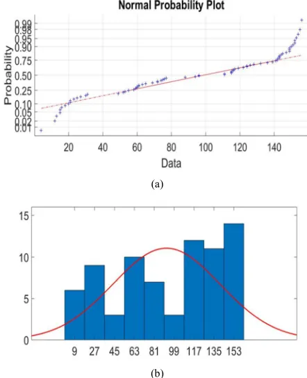
graphical methods such as histograms and cumulative distribution plot should be used in determining the segmentations of each variable [24]. Probability plots and histograms showing the variable data partitions for X1 and
2
X are illustrated in Figure 1 and Figure 2.
(a)
(b)
Figure 1. (a) Probability plot and (b) histogram for variable X1 of Ruspini
data set.
(a)
(b)
Figure 2. (a) Probability plot and (b) histogram for variable X2 of Ruspini
data set.
Figure 3. Partitions in variable data in X and 1 X forms a sixteen cluster 2 centers in Ruspini data set.
Figure 1 and Figure 2 X1 is partitioned as X11, X12, X13 and X14; X2 is partitioned as X21, X22, X23 and X24. This partitions forms sixteen cluster centers in Ruspini data set [21] as illustrated in Figure 3.
Segmentations in variables data forms the cluster centers are shown Figure 3. The 1st cluster center is obtained from
11
X andX21 variable data partitions. The 2nd cluster center is obtained from X12 andX21 variable data partitions. The 3rd
cluster center is obtained from X13 andX21 variable data partitions. The 4th cluster center is obtained from X14 and
21
X variable data partitions. The 5th cluster center is obtained
from X11 andX22 variable data partitions. The 6th cluster center is obtained from X12 and X22 variable data
partitions. The 7th cluster center is obtained from X13 and
22
X variable data partitions. The 8th cluster center is obtained
from X14 and X22 variable data partitions. The 9th cluster center is obtained from X11 and X23 variable data partitions. The 10th cluster center is obtained from X12 and X23 variable data partitions. The 11th cluster center is obtained from X13 and X23 variable data partitions. The 12th cluster center is obtained from X14 and X23 variable data partitions. The 13th cluster center is obtained from X11 and X24
variable data partitions. The 14th cluster center is obtained from X12 and X24 variable data partitions. The 15th cluster center is obtained from X13 and X24 variable data
partitions. The 16th cluster center is obtained from X14 and
24
X variable data partitions.
2.2. Computations for Total Number of Cluster Centers
The assumption of proposed method is that each column and row must have at least one cluster center in Figure 3. The method proposed by Servi and Erol [24] can be used to compute the minimum and maximum number of cluster centers, denoted by Cmin and Cmax, respectively in data set as
{ }
max min
C = ks s =1, ...,p (5)
and
max 1 p
s s
C k
=
=
∏
(6)where p denotes number of variables and k s denotes the number of partitions in each variable data for X1 and X2.
Thus, k1=k2=4 for Ruspini data set [21]. n×2 data matrix for
X is of the form X =X1 X2.
Partitions of X1 variable data in n1elements is of the form
11 12 1
13 14
X X X
X X
=
where X11 , X12 , X13 and X14 partitions
having n11, n12,n13 and n14 elements respectively. Thus,
1 11 12 13 14
n =n +n +n +n . Partitions of X2 variable data in n2
elements is of the form
21 22 2
23 24
X X X
X X
=
where X21, X22,X23
and X24 partitions having n21, n22,n23 and n24 elements respectively. Thus, n2 =n21+n22+n23+n24 . For the case considered, Cmin =max 4,4{ }=4 and Cmax =k k1 2=4.4=16. So the minimum number of cluster centers is 4 and the maximum number of cluster centers is 16 for Ruspini data set [21]. Partitions of variables data and cluster centers are illustrated in Figure 3.
Observations for variables can be assigned to partitions of variables using clustering algorithms such as k-means algorithm [25]. So variable data segmentations are obtained from both graphical methods: such as probability plots and histograms; and computational methods: such as mixture of univariate normal distributions and k-means. Variable data partitions and their sizes for variable X1 and X2 in Ruspini
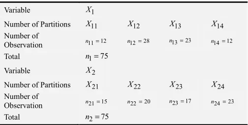
data set [21] are given in Table 3.
Table 3. Variable data segments and their sizes for X1 and X2 variables of
Ruspini data set.
Variable X1
Number of Partitions X11 X12 X13 X14
Number of
Observation n11=12 n12=28 n13=23 n14=12
Total n1=75
Variable X2
Number of Partitions X21 X22 X23 X24
Number of
Observation n21=15 n22=20 n23=17 n24=23
Total n2=75
Mean vectors and variance-covariance matrices of candidate cluster centers are obtained for construction of mixture models using variable data segmentations in multivariate data set or Ruspini data set [21]. General form of mean vectors in component probability density functions, thus bivariate normal probability density functions, corresponding to each candidate cluster center is of the form
1 µ
2
p i
q
µ µ
=
for
1, ...,
i = k and k =1, ...,16, ,p q=1, ..., 4 (7)
where µ1p and µ2q corresponds to X11, X12 , X13 and
14
X segments for X1, and X21 , X22 , X23 and X24
segments for X2, respectively.
component probability density functions, thus bivariate normal probability density functions, corresponding to each candidate cluster center is of the form
2
1 2 1
Σ
2
2 1 2
i p q p
i
i q p q
σ ρ σ σ
ρ σ σ σ
=
for i=1, ...,k and k =1, ...,16 (8)
where σ1p and σ2q corresponds to X11, X12 , X13 and
14
X segments for X1, and X21 , X22 , X23 and X24
segments for X2 , respectively. Correlations between
partitions of variables are defined as ρ1 ,2p q =Corr(X1p, X2q).
Mean vectors and variance-covariance matrices are used in construction of mixture models for mixture model clustering using variable data segmentation and model selection.
2.3. Computations for Total and Possible Number of Mıxture Models Usıng Cluster Centers
The total number of mixture models for cluster centers, obtained from variable data segmentation and denoted by
Total
M , for Ruspini data set [21] can be computed by the relation proposed by Erol [14] as follows
max 2C 1
Total
M = − (9)
where Cmax as in (6). Minus one term is used to eliminate the case of no cluster center.
Total
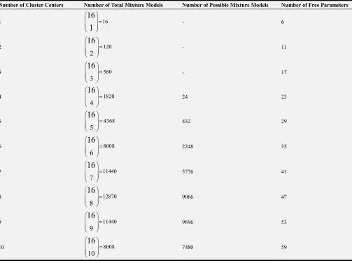
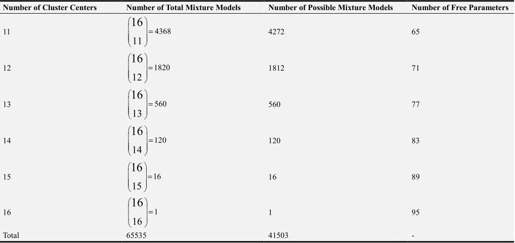
M can be obtained as MTotal =216− =1 65535 for Ruspini data set [21]. The number of cluster centers, the number of total mixture models, the number of possible mixture models and the number of free parameters in mixture models are given in Table 4. Some cases of mixture models does not satisfy the assumption which is each column and row has at least one cluster center, so they are eliminated. The remaining mixture models are called candidate mixture models. The number of possible or candidate mixture models can be computed using the relation formula proposed by Cheballah et al. [26] as
( )( )
( , , , ) ( 1) ( 1)
0 0
n i n m j m n i m j f n m s k
i j k
i j
− −
∑ ∑
= − −
= = (10)
where n and m corresponds to number of partitions in variables X1 and X2 respectively. Indices i and j are used for the number of cluster centers. k denotes the cases for the number of cluster centers in mixture models.
Table 4. The number of cluster centers, the number of total mixture models, the number of possible mixture models and the number of free parameters.
Number of Cluster Centers Number of Total Mixture Models Number of Possible Mixture Models Number of Free Parameters
1
16
161
=
- 6
2 120
2
16
=
- 11
3 560
3
16
=
- 17
4 1820
4
16
=
24 23
5 4368
5
16
=
432 29
6 8008
6
16
=
2248 35
7 11440
7
16
=
5776 41
8 12870
8
16
=
9066 47
9 11440
9
16
=
9696 53
10 8008
10
16
=
Number of Cluster Centers Number of Total Mixture Models Number of Possible Mixture Models Number of Free Parameters
11 4368
11
16
=
4272 65
12 1820
12
16
=
1812 71
13 560
13
16
=
560 77
14 120
14
16
=
120 83
15 16
15
16
=
16 89
16 1
16
16
=
1 95
Total 65535 41503 -
2.4. Binary String Representation Of Possible Mixture Models Using Cluster Centers
Mixture model clustering using variable data segmentation and based on model selection uses a genetic algorithm. The genetic algorithm is used to calculate the information criteria of each candidate mixture model. String representation of each candidate model consists of 1 and 0 digits. In Table 5 the
zeros and/or the ones represent whether the centers used in construct of the mixture model or not. Binary string representations of possible mixture models with each corresponding to one of 41503 possible models numbers is given in Table 4. For instance the binary string representation of the saturated mixture model that uses all cluster centers is given in Table 5.
Table 5. All sixteen cluster centers represented by one (1) means that all constructed the model.
1 2 3 4 5 6 7 8 9 10 11 12 13 14 15 16
1 1 1 1 1 1 1 1 1 1 1 1 1 1 1 1
2.5. List Of Possible Mixture Models Using Cluster Centers
Each binary string representation of candidate mixture model corresponds to one of 41503 possible mixture models.
General form of mixture model with k (4≤k≤16) components and having binary string representation is of the form as
( ) ( ) ( ) ( ) ( ) ( )
1
( ; , ) ( ; , )
k
u u u u u u
i i i i
i
f xµ π f x µ
=
Σ =
∑
Σ for u=1, ..., 41503 (11)where mixing proportions for component density function is of the form
( ) 4
1
u i
i
l l
π π
π =
∑
=
for u=1, ..., 41503 (12)
mean vector for component density function is of the form:
( ) 1 ( )
( ) 2
u p u
i u
q
µ µ
µ
=
for u=1, ..., 41503 (13)
variance-covariance matrices for component density function is of the form:
( )2 ( ) ( ) ( )
( 1 ) 1 ,2 1 2
( )
( ) ( ) ( ) ( ( ) 2)
2 ,1 2 1 2
u u u u
p p q p q
u
i u u u u
q p q p q
σ ρ σ σ
ρ σ σ σ
Σ =
for u=1, ..., 41503 (14)
where component density function is probability density function for bivariate normal distribution.
There are 24 possible mixture models with four components (k=4) of the form as in (11). Parameters in the mixture models are πi( )u , µi( )u and Σ( )iu as in (12), (13) and (14) respectively with u=1, ..., 24. There are 432 possible mixture
models with five components (k=5) of the form as in (11).
248 possible mixture models with six components (k=6) of the form as in (11). Parameters in the mixture models are πi( )u ,
( )u i
µ and Σi( )u as in (12), (13) and (14) respectively with
457, ..., 2704
u= . There are 5776 possible mixture models with
seven components (k=7) of the form as in (11). Parameters in
the mixture models are πi( )u , µi( )u and Σi( )u as in (12), (13) and (14) respectively with u=2705, ..., 8480. There are 9066 possible mixture models with eight components (k=8) of the
form as in (11). Parameters in the mixture models are πi( )u ,
( )u i
µ and Σ( )iu in (12), (13) and (14) respectively with
8481, ...,17546
u= . There are 9696 possible mixture models with nine components (k=9) of the form as in (11). Parameters in the mixture models are πi( )u , µi( )u and Σ( )iu in (12), (13) and (14) respectively with u=17547, ..., 27242 . There are 7480
possible mixture models with ten components (k=10) of the
form as in (11). Parameters in the mixture models are πi( )u ,
( )u i
µ and Σ( )iu in (12), (13) and (14) respectively with
27243, ..., 34722
u= . There are 4272 possible mixture models with eleven components (k=11) of the form as in (11).
Parameters in the mixture models are πi( )u , µi( )u and Σ( )iu in (12), (13) and (14) respectively with u=34723, ..., 38994. There
are 1812 possible mixture models with twelve components (k=12) of the form as in (11). Parameters in the mixture
models are πi( )u , µi( )u and Σ( )iu in (12), (13) and (14) respectively with u=38995, ..., 40806. There are 560 possible mixture models with thirteen components (k=13) of the form as in (11). Parameters in the mixture models are πi( )u , µi( )u
and Σ( )iu in (12), (13) and (14) respectively with
40807, ..., 41366
u= . There are 120 possible mixture models with
fourteen components ( k=14 ) of the form as in (11). Parameters in the mixture models are πi( )u , µi( )u and Σ( )iu in (12), (13) and (14) respectively with u=41367, ..., 41486. There
are 16 possible mixture models with fifteen components (k=15) of the form as in (11). Parameters in the mixture models are πi( )u , µi( )u and Σ( )iu in (12), (13) and (14) respectively with u=41487, ..., 41502 . There is 1 possible
mixture model with sixteen components (k=16) of the form as in (11). Parameters in the mixture models are πi( )u , µi( )u
and Σi( )u in (12), (13) and (14) respectively with u=41503.
2.6. Estimation of Parameters for Possible Mixture Models Using Cluster Centers
Mixture model clustering using variable data segmentation and based on model selection, proposed in this study, is a data mining method. The method developed for mixture model clustering has its own genetic algorithm explained in the
previous sections. Since variable data segmentation applied to each variable in the data set; mean vectors, variance-covariance matrices and mixing proportions for each component of possible mixture models can be estimated from the sample. The complexity of mixture model clustering using variable data segmentation and based on model selection is less than other clustering methods. Each binary string representation, as in Table 5, corresponds to one of 41503 possible mixture models of the form as in (11).
The estimate of mixing proportions for component density functions are of the form
( ) 1 n u i i k nl l π = ∑ =
⌢ for u=1, ..., 41503 (15)
where k denotes the number of components in the possible mixture models. The estimate of mean vectors for component density functions are of the form
( ) 1 ( ) ( ) 3 u x p u i u x q µ =
⌢ for u=1, ..., 41503 (16)
The estimate of variance-covariance matrices for component density functions are of the form
( ) 2 ( ) ( ) ( )
(1 ) 1 ,2 1 2
( )
( ) ( ) ( ) ( ( ) 2)
2 ,1 2 1 2
u u u u
Sp rp qSpS q u
i u u u u
rq pS qSp S q
Σ = ⌢
for u=1, ..., 41503 (17)
Parameter estimate π⌢i( )u , ( )u
i
µ⌢ and ( )u
i Σ⌢
of 24 possible mixture models with four components (k=4) as in (15), (16) and (17) respectively with u=1, ..., 24 . Parameter estimate
( )u i
π⌢ , ( )u
i
µ⌢ and ( )u
i Σ⌢
of 432 possible mixture models with five components (k=5) as in (15), (16) and (17) respectively
with u=25, ..., 456. Parameter estimate π⌢i( )u , ( )u
i
µ⌢ and ( )u
i Σ⌢
of 2248 possible mixture models with six components (k=6) as in (15), (16) and (17) respectively with u=457, ..., 2704.
Parameter estimate π⌢i( )u , ( )u
i
µ⌢ and ( )u
i Σ⌢
of 5776 possible mixture models with seven components (k=7) as in (15), (16) and (17) respectively with u=2705, ..., 8480. Parameter estimate
( )u i π⌢ , ( )u
i
µ⌢ and ( )u
i Σ⌢
of 9066 possible mixture models with eight components (k=8) as in (15), (16) and (17) respectively with u=8481, ...,17546. Parameter estimate π⌢i( )u , ( )u
i µ⌢ and
( )u i Σ⌢
of 9696 possible mixture models with nine components ( k=9 ) as in (15), (16) and (17) respectively with
17547, ..., 27242
u= . Parameter estimate π⌢( )iu , ( )u
i
µ⌢ and ( )u
i Σ⌢
of 7480 possible mixture models with ten components (k=10) as in (15), (16) and (17) respectively with u=27243, ..., 34722.
Parameter estimate π⌢i( )u , ( )u
i
µ⌢ and ( )u
i Σ⌢
(16) and (17) respectively with u=34723, ..., 38994. Parameter
estimate π⌢i( )u , ( )u
i
µ⌢ and ( )u
i Σ⌢
of 1812 possible mixture models with twelve components (k=12) as in (15), (16) and (17) respectively with u=38995, ..., 40806. Parameter estimate
( )u i
π⌢ , ( )u
i
µ⌢ and ( )u
i Σ⌢
of 560 possible mixture models with thirteen components ( k=13 ) as in (15), (16) and (17) respectively with u=40807, ..., 41366. Parameter estimate π⌢i( )u ,
( )u i
µ⌢ and ( )u
i Σ⌢
of 120 possible mixture models with fourteen components (k=14) as in (15), (16) and (17) respectively with
41367, ..., 41486
u= . Parameter estimate π⌢( )iu , ( )u
i
µ⌢ and ( )u
i Σ⌢
of 16 possible mixture models with fifteen components (k=15) as in (15), (16) and (17) respectively with u=41487, ..., 41502.
Parameter estimate π⌢( )iu , ( )u
i
µ⌢ and ( )u
i Σ⌢
of 1 possible mixture model with sixteen components (k=16) as in (15), (16) and (17) respectively with u=41503.
2.7. Computation of Information Criteria for Possible Mixture Models
Likelihood function for the mixture of multivariate normal densities is defined as
(π, µ, Σ) (x ;θ) π (x ;µ ,Σ )
1 1 1
n n k
L f j i if j i i
j j i
∏ ∏
= = ∑
= = = (18)
and log-likelihood function for the mixture of multivariate normal densities is computed as
log (π, µ, Σ) log( π (x ; µ , Σ ))
1 1
n k
L i if j i i
j i
∑ ∑
=
= = (19)
The Maximum Likelihood Estimation method is used in mixture distributions to obtain the parameters in the data set [27]. Log-likelihood function values for possible mixture of bivariate normal densities are computed using the estimated values of π⌢i( )u , ( )u
i
µ⌢ and ( )u
i Σ⌢
for the Ruspini data set [21].
Akaike’s information criterion (AIC) can be computed by
ˆ ˆ ˆ
AIC=-2 log (π, µ, Σ)L +2d (20)
Bayesian information criterion (BIC) can be computed by
ˆ ˆ ˆ
BIC=-2 log (π, µ, Σ)L +dlogn (21)
where log (π, µ, Σ)L ˆ ˆ ˆ is the value of log-likelihood function for
possible mixture of multivariate normal densities; d is the
number of free parameters in possible mixture of bivariate normal densities and n is the number of observation. The number of free parameters in possible mixture of multivariate normal densities d can be computed by:
( )1 ( 1)
2
p d= k− +kp+kp +
(22)
where k is the number of components, p is the number of variables or dimension in mixture model [5]. Log-likelihood function, AIC and BIC values are computed from partitions of variables data using mean vectors and variance-covariance matrices. Log-likelihood function, AIC and BIC values will be used as criteria for selecting the best mixture model of bivariate normal densities. All calculations are performed using MATLAB.
2.8. Selection of The Best Model In a Set of Possible Mixture Models
Selection of the best mixture model among possible mixture of bivariate normal densities for the Ruspini data set [21] according to the information criteria is performed using the values of log-likelihood function, AIC and BIC. The mixture model having maximum Log-likelihood function value and, the mixture model having minimum AIC and BIC values is selected as the best mixture model among the possible 41503 mixture models. The string representation of the best mixture model is given in Table 6.
Table 6. The best mixture model string representation.
1 2 3 4 5 6 7 8 9 10 11 12 13 14 15 16
0 0 1 0 1 0 0 0 0 0 0 1 0 1 0 0
The number of components, log-likelihood, AIC and BIC values of the best mixture model is given in Table 7.
Table 7. Log-likelihood, AIC and BIC values of the best mixture model.
Number of Component Log-l AIC BIC
4 -1560.4 3124.7 3130.0
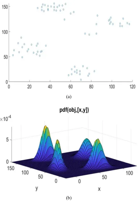
The best mixture model is selected as the mixture of four component bivariate normal densities for Ruspini data set [21]. The best mixture model is the 12th mixture model among
(a)
(b)
Figure 4. (a) The scatter plot and (b) The surface plot of the best mixture model.
3. Conclusions
In this study, a new data mining method using genetic algorithm for mixture model clustering based on variable data segmentation and model selection was developed and performed on Ruspini data set. In the developed genetic algorithm, we calculated the number of candidate cluster centers and structures resulting from segmentation of heterogeneous variables. All mixture models that can be formed from these candidate cluster centers and the number of possible mixture models that are appropriate for the hypothesis were calculated. Possible mixture models corresponding to candidate cluster centers were generated using genetic algorithm. In order to be able to compute possible mixture models, string representation of each possible mixture model was obtained. To be used in calculations, unknown parameters for possible mixture of bivariate normal distributions were calculated from the sample. The information complexity of the proposed mixture model clustering is less than other clustering methods that is why algorithms such as Expectation and Maximization (EM) is not used in computations for estimation of parameters. According to the calculated values thus, log-likelihood, AIC and BIC, the best mixture model that matches the best data clustering structure for Ruspini data set was decided.
It can be heuristically stated that the partitions in the heterogeneous variable data affects and determines the number and structure of clusters in data set with no matter what the number of the variable in data is. The clustering method proposed in this study is developed specially for model based clustering of big data.
As a future work, the proposed method will be applied on human brain studies. The study will cover, the number of human brain function centers, magnitude of these brain function centers, correlation between these brain function centers, and constructing mixture models for these brain function centers of human behaviours and activity movements. Furthermore, the method can be applied on robotics, artificial intelligence and logical circuit design for decision making applications.
References
[1] McLachlan, G. J. and Peel, D. (2000). Finite Mixture Models. Wiley, New York.
[2] Fraley, C. and Raftery, A. E. (2002). Model-Based Clustering, Discriminant Analysis, and Density Estimation. Journal of the American Statistical Association, 97, 611-631.
[3] Fraley, C. and Raftery, A. E. (1998). How Many Clusters? Which Clustering Method? Answers via Model-Based Cluster Analysis. The Computer Journal, 41, 578-588.
[4] Bozdogan, H. (1994a). Choosing the number of clusters, subset selection of variables, and outlier detection in the standart mixture model cluster anlysis. Invited paper in New Approaches in Classification and Data Ana lysis, E. Diday et al. (Eds.), Springer-Verlang, New York, pp. 169-177.
[5] Bozdogan, H. (1994b). Mixture-Model Cluster Analysis Using Model Selection Criteria And A New Informational Measure Of Complexity. In Multivariate Statistical Modeling, Vol. 2, H. Bozdogan (ed.), Kluwer Academic Publishers, Dordrecht, the Netherlands, 1994, pp. 69-113.
[6] Soffritti, G. (2003). Identifying multiple cluster structures in a data matrix. Communications in Statistics, Simulation & Computation, Vol. 32, Issue 4, pp. 1151-1181.
[7] Bozdogan, H. (2004). Intelligent Statistical Data Mining with Information Complexity and Genetic Algorithms. In Statistical Data Mining & Knowledge Discovery, H. Bozdogan (Ed.), Chapman & Hall/CRC, pp. 15-56.
[8] McLachlan, G. J. and Chang, S. U. (2004). Mixture Modelling for Cluster Analysis. Statistical Methods in Medical Research 13, 347-361.
[9] Galimberti, G. and Soffritti, G. (2007). Model-based methods to identify multiple cluster structures in a data set. Computational Statistics and Data Analysis. doi 10.1016/j.csda.2007.02.019.
[10] Durio, A. and Isaia, E. D. (2007). A quick procedure for model selection in the case of mixture of normal densities. Computational Statistics and Data Analysis. 51, 5635-5643. [11] Scrucca, L. (2010). Dimension reduction for model-based
[12] Seo, B. and Kim, D. (2012). Root selection in normal mixture models. Computational Statistics and Data Analysis. 56, 2454-2470.
[13] Fraley, C., Raftery, A. E., and Scrucca, L. (2012). Normal mixture modeling for model-based clustering, classification, and density estimation. Department of Statistics, University of Washington, Available online at http://cran.r-project. org/web/packages/mclust/index.html. Accessed September, 23, 2012.
[14] Erol, H. (2013). A model selection algorithm for mixture model clustering of heterogeneous multivariate data. In Innovations in Intelligent Systems and Applications (INISTA), 2013 IEEE International Symposium. pp. 1-7.
[15] Huang, T., Peng, H., and Zhang, K. (2013). Model Selection for Gaussian Mixture Models. arXiv preprint arXiv: 1301.3558. [16] McLachlan, G. J. and Krishnan, T. (1997). The EM Algorithm
and Extensions. New York, Wiley.
[17] Galimberti, G., and Soffritti, G. (2013). Using conditional independence for parsimonious model-based Gaussian clustering. Statistics and Computing, 23 (5), 625-638. [18] McLachlan, G. J., and Rathnayake, S. (2014). On the number of
components in a Gaussian mixture model. Wiley Interdisciplinary Reviews: Data Mining and Knowledge Discovery, 4 (5), 341-355.
[19] Wei, Y. and McNicholas, P. D. (2015). Mixture model averaging for clustering. Adv Data Anal Classif (2015) 9: 197– 217. DOI 10.1007/s11634-014-0182-6.
[20] Bouveyrona, C. and Brunet-Saumardb, C. (2014). Model-based clustering of high-dimensional data: A review Computational Statistics and Data Analysis. 71, 52–78.
[21] Maitra, R., and Melnykov, V. (2010) Simulating data to study performance of finite mixture modeling and clustering algorithms. Journal of Computational and Graphical Statistics, 19 (2), 354-376.
[22] Akaike, H. (1974). A new look at the statistical model identification. IEEE Transactions on Automatic Control 19 (6): 716–723.
[23] Schwarz, G. (1978). Estimating the dimension of a model, Ann. Statist. 6 pp. 461–464.
[24] Servi, T. and Erol, H. (2007). On Total Number of Candidate Component Cluster Centers and Total Number of Candidate Mixture Models In Model Based Clustering. Selçuk Journal of Applied Mathematics Vol. 8. No. 2. pp. 57-69.
[25] Kaufman, L. and Rousseeuw, P. (1990). Finding Groups in Data: An Introduction to Cluster Analysis. New York: Wiley-Interscience.
[26] Cheballah, H., Giraudo, S. And Maurice, R. (2015) Combinatorial Hopf Algebra Structure On Packed Square Matrices. Journal of Combinatorial Theory Series A, Volume 133, Issue C, Pages 139-182. doi: 10.1016/j.jcta.2015.02.001. [27] Erişoğlu Ü., Erişoğlu M., and Erol H., “Mixture Model
Approach To The Analysis Of Heterogeneous Survival Data,” Pakistan Journal Of Statistics, vol. 28, no. 1, pp. 115–130, Jan. 2012.
[28] Akogul, S., & Erisoglu, M. (2016). A Comparison of Information Criteria in Clustering Based on Mixture of Multivariate Normal Distributions. Mathematical and Computational Applications, 21 (3), 34–0.
[29] Akogul, S., & Erisoglu, M. (2017). An Approach for Determining the Number of Clusters in a Model Based Cluster Analysis. Entropy, 19 (9), 452–0.
[30] Celeux, G., Fruewirth-Schnatter, S., & Robert, C. P. (2018). Model selection for mixture models-perspectives and strategies. arXiv preprint arXiv: 1812.09885.