Article
Application of the Lagrangian Meshfree Approach to Modelling
of Batch Crystallisation: Part II—An Efficient Solution of
Integrated CFD and Population Balance Equations
Dragan D. Nikolić * and Patrick J. Frawley
Synthesis and Solid State Pharmaceutical Centre, University of Limerick, Limerick V94 T9PX, Ireland; [email protected]
* Correspondence: [email protected] or [email protected]
distribution was captured and compared to the ideal mixing case. The simulation results from the DPB and MOCH methods were compared in terms of computational requirements and accuracy and MOCH selected as computationally more efficient and accurate.
Keywords: CFD; SPH; population balance; NVidia CUDA; OpenMP
1. Introduction
A large number of engineering fields such as chemical, petrochemical, pharmaceutical, microelectronics, aerosol formation, food processing, colloid chemistry, growth of cell populations and atmospheric physics involve a dynamic evolution of a distribution of particles. The performance of many industrial downstream processes is directly affected by particle characteristics and product qualities such as morphology, bulk density, average particle size, filterability and dry solid flow properties are directly related to the crystal size distribution (CSD). Therefore, the CSD is one of the most important process performance parameters. The dynamical behaviour of particles can be best described by population balance equations (PBE) (Ramkrishna, 2000). The population balance modelling framework provides a deterministic description of the dynamic evolution of the crystal size distribution by forming a balance to calculate the number of crystals in the crystalliser. Since all the above-mentioned processes are largely affected by hydrodynamics the population balance equations are often coupled with computational fluid dynamics (CFD) modelling to correctly predict the key process performance indicators.
Galerkin methods (Singh and Ramkrishna, 1977; Sporleder et al., 2011; van den Bosch and Padmanabhan, 1974; Nigam and Nigam, 1980; Roussos et al., 2005), and e) Dynamic Monte Carlo simulation (DMC) (Haseltine and Rawlings, 2005; Rosner et al., 2003). The two most often used techniques are the standard method of moments and the quadrature method of moments. The method of moments is based on the idea of tracking only the moments of the crystal size distribution, rather than the entire distribution. In addition, there were some efforts to use combined methods to achieve a computationally efficient technique for the estimation of the crystal size distribution, such as combined QMOM and MOCH (Aamir et al., 2009). The common problem encountered with the method of moments is that the CSD is lost and needs to be reconstructed from its distribution moments. Many reconstruction techniques were developed however, no unified technique for reconstruction of a complete distribution from a finite number of moments is available in literature due to the fact that mathematically all the distribution moments up to infinity are required to achieve an accurate reconstruction (John et al., 2007).
2. Population Balance modelling
The mathematical description of the evolution of particle properties during a process can be written as (Ramkrishna, 2000):
(1)
where n(L,t) is the number density function, L is the internal property such as characteristic length, volume, mass etc., G(L,t) is growth rate and s(L,t,n) is the generation/depletion rate. The term s(L,t,n) can include nucleation, breakage, agglomeration, aggregation, attrition and other phenomena that contribute to the change of the number density function. Often, these terms are defined as integral functions making the whole equation (1) an integro partial-differential equation. There is a large number of methods to solve the population balance equations numerically and in some case analytically, as already discussed in the previous section. In this work the methods for solution of population balance equations that are capable to preserve the full crystal size distribution are of a special interest. The most suitable in terms of implementation cost and computational requirements are the well known discretised population balance (DPB) and the method of characteristics (MOCH). The methods are briefly described in the subsequent sections.
2.1 Discretised population balance method (DPB)
The most commonly used direct numerical solution approaches to population balance equations are finite-difference, finite-element and finite-volume discretisation techniques. The equation (1) is hyperbolic in its nature and a typical problem is accurate tracking of sharp fronts in the particle distribution since the differential equation is not valid at discontinuities, which lead to numerical diffusion and non-physical oscillations (LeVeque, 2002). The high-resolution finite-volume methods (LeVeque, 2002) have been developed to address these problems. Finite volumes allow direct satisfaction of conservation laws while cell-centering leads to a natural situation where domain boundaries coincide with cell faces (Koren, 1993).
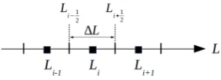
The DPB equations are obtained by discretising the domain L (particle size) into N
cells/elements as given in Fig. 1. Applying the cell-centered finite volume scheme on the one-dimensional population balance equation we get (Koren, 1993):
where the first integral term represents the volume-average number density in every cell:
( 3)
Since the discretisation of the source term should be consistent with the discretisation of the advection term to avoid numerical problems (Koren, 1993) the new source term integral S is introduced:
(4)
Replacing the new terms in the integral form in equation (2) and integrating in every cell i, we get:
(5)
where the term (Gn-S) denotes an extended advective flux while the half-integer indices i-1/2
and i+1/2 refer to the cell faces between cell centres Li-1 – Li, and Li – Li+1, respectively;
consequently, the terms (Gn)i-1/2 and (Gn)i+1/2 denote the cell-face fluxes of the element i at
its left and right edge, respectively. The accuracy of the numerical scheme is determined by the way in which the extended advective fluxes are calculated. Assuming that the flow is in
positive L-direction: and applying the van Leer
piecewise polynomial κ-interpolation (van Leer, 1985) we get:
(6)
(7) where φ is a flux limiter function and r represents the upwind ratio of two consecutive solution gradients (Koren, 1993):
(8)
There are a large number of flux limiter functions and a list of the most frequently used ones is given in Table 1. The limiter functions must satisfy certain conditions such as they must lay inside or at the boundary of the Sweby's monotonicity domain (Sweby, 1984). Limiter functions used in this work in relation to 2nd order total variation diminishing
(TVD) region are given in Fig. 2. Since the piecewise polynomial interpolation cannot be applied around and at boundaries (Koren, 1993) the equation (6) must be modified accordingly: a) the flux at the inflow boundary L1/2 is known exactly through the boundary condition, b) at L3/2 only the central interpolation with κ = 1 can be consistently applied, and c) at the outflow boundary Ln+1/2 only the fully one-sided upwind scheme κ = -1 can be applied. The full set of equations can be found in Koren (1993).
2.2 Method of characteristics (MOCH)
The generic partial differential equation (1) can be reduced to a system of ordinary differential equations by finding the characteristic curves in the L – t plane (Aamir et al., 2009). The L – t plane is given in a parametric form by L = L(z) and t = t(z) where the parameter z gives the measure of the distance along the characteristic curve. For the partial differential equation (1), the characteristic curves are given parametrically:
(9)
such that the following system of ODEs is satisfied:
(10)
(11)
(12)
with the following initial conditions:
(13)
(15)
The equation (1) must be linear or quasi-linear, that is the growth rate can be size-dependent but must not depend on any derivative. Since the number density function is now a function of L(z) and t(z), applying the chain rule:
(16)
we get:
(17)
Comparing equations (16) and (18) it can shown that (Aamir et al., 2009):
(18) and consequently, the characteristic equations can be described by the following system of equations:
(19)
(20)
To obtain the dynamic evolution of the crystal size distribution the system of equations (19‒20) has to be integrated for different initial values L0 and n(L0,0), accompanied with growth and generation/depletion rates. Typically, they are a function of supersaturationand can be obtained from the mass balance for the solute using the moment transformation of equation (1). Aamir et al. (2009) used the combined quadrature method of moments with method of characteristics, however, only the change of the total mass of crystals is required to form the solute mass balance. For the size-independent growth-only process the system (19‒20) simplifies to:
(21)
(22)
Phenomena that cause the change of the distribution like primary/secondary nucleation, breakage, agglomeration etc. need a special treatment. Regarding the primary nucleation, the method requires that a new characteristic line is added every time step. However, in this work it is assumed that crystals in the characteristic line with the smallest crystal size L=L0
size in the CSD) the size of the crystals in the first characteristic line is set to L0+ΔL and the
new characteristic line inserted at the beginning with the size L0. From that point in time,
the crystals in the characteristic line with size L0+ΔL are allowed to grow according to the
equations (19‒20). This way, the computational and memory requirements are kept low. Secondary nucleation, breakage and agglomeration require a mathematical procedure to maintain internal consistency with regard to the desired moments of the distribution (Kumar and Ramkrishna, 1996a, 1996b). In this work, the fixed pivot technique proposed by Kumar and Ramkrishna (1996a) is selected and implemented. The pivoting technique is used to numerically preserve two properties of the distribution: the total number and mass of crystals. In addition, the identical procedure is applied at the end of the simulation to assemble the final crystal size distribution from local distributions available in every particle.
3. Integrated Smoothed Particle Hydrodynamics and Population Balance model
Two different algorithms for coupled SPH and population balance have been developed in this work: a) both SPH and population balance equations integrated on GPU, b) SPH equations integrated on GPU while population balance equations integrated on CPUs using the OpenMP interface. The following basic assumptions have been made: the solid phase is assumed to closely follow the flow field that is the Stokes number is sufficiently low, the presence of the solid phase does not affect the flow field, the growth rate is independent of crystal size, and the perfect micromixing is assumed to exist in each fluid particle.
The first algorithm is an extension of the SPH model (Nikolic and Frawley, 2015) by using additional transport equations. Three scalar transport equations were added: the heat conduction (between fluid particles and between the fluid particles and the reactor wall), the mass diffusion (concentration of dissolved crystals) and a set of population balance equations (either DPB or MOCH). The heat conduction and mass diffusion equations were adopted from the work of Monaghan et al. (2005):
(23)
(24)
where λi is thermal conductivity and Di is mass diffusion coefficient. Similar to the pressure
ensure that the flux will be continuous even when the conductivity is discontinuous (at the phase interfaces; here, at the fluid-wall interface). The SPH model of a stirred tank is implemented in c++ using Fluidix software (MacDonald, 2014) and identical to that described in Nikolic and Frawley (2015). The simulation procedure consists of the initialization phase and the main SPH loop. First, triangular surface meshes are generated for stirred tank walls, baffles and a stirrer shaft with impellers. These meshes can be directly loaded into the Fluidix software. Then, uniformly distributed fluid particles of the specified size are generated inside the whole volume of the tank and the particles that are positioned inside the baffles and stirrer meshes are removed. An excess number of particles from the top of the reactor, up to the prescribed volume, is also removed. Now, “wall” particles are created at all mesh vertices. The SPH main loop is implemented in a standard fashion. First, a density of all particles is estimated and internal forces evaluated such as the pressure gradient, shear forces, gravity and the surface tension. Stirrer mesh and its wall particles are rotated and the forces between impeller and fluid particles are calculated. The system is now integrated in time using the second order Verlet scheme and particle-mesh collisions processed to update particle positions. This procedure is repeated until the defined time horizon is reached.
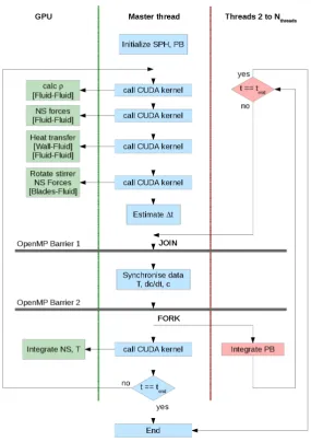
The second algorithm is more complex. The computational procedure is divided into three parts: 1) the master thread – a controlling thread that manages the calls to CUDA kernels and controls a team of OpenMP threads, 2) the team of (Nthreads-1) threads used to integrate
population balance in parallel, 3) GPU used to calculate particle interactions and integrate Navier-Stokes, heat and mass balance equations. The solution algorithm is presented in Fig. 3. First, the system is initialized in the master thread in an identical fashion as in the first algorithm. Next, the master thread repeatedly calls CUDA kernels to calculate the forces and gradients in Navier-Stokes, heat and mass balance equations and to estimate the time step. All other threads are idle. When the master thread finishes the work all threads are joined at the OpenMP barrier 1. Next, the solute concentration in particles is copied from the main memory to GPU and the temperature and the concentration gradient in particles copied from GPU to the main memory by the master thread. All other threads are idle. When the master thread is done with the memory synchronisation all threads are joined at the OpenMP barrier 2. Now, (Nthreads-1) population balance threads are forked to integrate
after the integration stage, all threads check whether the time horizon has been reached and exit if it has. If the time for integration of population balance equations is lower then combined time to calculate the forces and gradients and integrate the Navier-Stokes, heat and mass balance equations the total simulation time should be equal to the SPH-only simulation and the combined algorithm should be faster than the initial GPU-only algorithm. However, this is not the case in reality since some time is always spent on thread scheduling, memory copy between the GPU and the main memory and waiting at barriers. Therefore, the algorithm is always somewhat slower then the SPH only simulation. The benchmarks and a detailed discussion on computational requirements is given in section 4.4.
4. Case Studies
4.1 High-resolution schemes
In this section the simulation results obtained by using the high-resolution scheme for solution of DPB equations were compared to the analytical solutions for different cases using the numerical examples from Qamar et al. (2006). A range of different flux limiter functions given in Table 1 have been used in all tests. All models in this section were developed in Python using DAE Tools software (Nikolic, 2014). The quality of prediction of different flux limiters was assessed by calculating the p-norms in the Lp space:
(25)
where nHR is the number density function from the high-resolution scheme and nAnalytical is the number density function from the analytical solution. Two error norms have been used:
a) L1-norm: (26)
b) L2-norm: (27)
4.1.1 Size-independent growth I
are smooth, sharp fronts occur very often during the primary nucleation, especially in anti-solvent crystallisations, due to high supersaturation values when a burst in the number density function of nearly zero-sized crystals occurs. Here, the growth-only crystallisation process was considered with the constant growth rate of 1μm/s and the following initial number density function:
(28)
The crystal size distribution in the size range of [0, 100]μm discretised into 100 elements was used. The analytical solution in this case is equal to the initial profile translated right in time by a distance Gt (the growth rate multiplied by the time elapsed in the process):
(29)
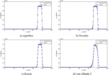
This problem is a good numerical benchmark because it is a combination of a sharp step function in the distribution and a very high growth rate. If the method works under these extreme conditions one can expect very good numerical results in the real problems without sharp fronts and with lower growth rates (Qamar et al., 2006). The simulations were performed using the I-order upwind, II-order central, and high-resolution schemes with different flux limiters and the results compared to the analytical solution. The number density functions for the I-order upwind and II-order central are shown in Fig. 4 and the best three high-resolution schemes (a-c) and the worst one (d) are presented in Fig. 5. L1
and L2 norms for high-resolution schemes are given in Table 2. As expected, the I-order
upwind scheme produces the solution with a very high numerical diffusion while the II-order central scheme produces non-physical oscillation in the presence of sharp fronts. The high-resolution schemes suppressed the numerical diffusion, non-physical oscillations and negative values in the solution to a different degree. In this case, the superbee, Sweby and Koren flux limiters showed the best prediction compared to the analytical solution and the superbee outperformed all the rest in terms of both L1 and L2 error tests.
4.1.2 Size-independent growth II
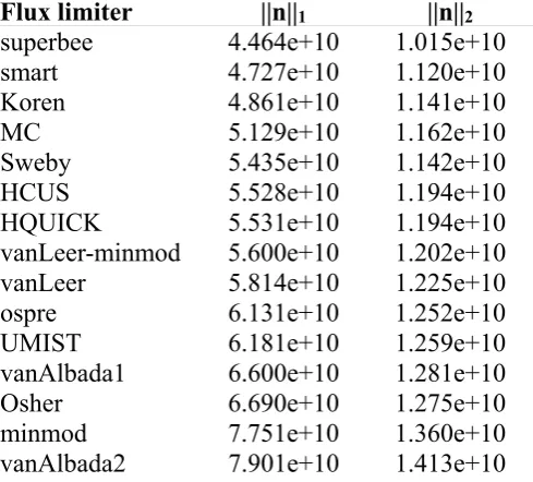
(30) The first region is a square step with a sharp discontinuity, the second region is a cosine-squared wave with the discontinuities at each side, the third region is a semi-ellipse with a combination of sharp and gradual changes in gradient, and the last region represents a narrow Gaussian distribution (σ = 0.778ΔL) with a very sharp peak. The results are compared to the analytical solution: the best three high-resolution schemes (a-c) and the worst one (d) are presented in Fig. 6. L1 and L2 norms for high-resolution schemes are
given in Table 3. Again, the high-resolution schemes suppressed the numerical diffusion, non-physical oscillations and negative values in the solution to a different degree. Overall, the superbee, smart and Koren flux limiters showed the best prediction compared to the analytical solution and the superbee again produced the best prediction in both error tests. The results in the first three regions are fairly good for all flux limiters; however, a certain degree of numerical diffusion is still present in all of them. In the most challenging fourth region we can clearly observe the limitations of discretisation schemes. The very sharp peaks commonly occur at the beginning of the distribution during an intense nucleation. The solution to this phenomena would be a very fine grid for the smallest sizes in the distribution or some sort of an adaptive grid. However, both approaches demand a much higher computational power to successfully resolve this kind of discontinuities.
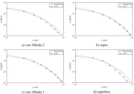
4.1.3 Size-dependent growth
(31)
and the crystal size distribution in the size range of [0, 1]μm discretised into 100 elements. The analytical solution in this case and is given by:
(32)
where G0 is a constant (0.1μm/s), Lmean is the distribution mean size (0.01μm) and N0 is the total number of particles in the distribution (100). The initial number density function is given by:
(33)
The results are compared to the analytical solution: the best three high-resolution schemes (a-c) and the worst one (d) are presented in Fig. 7 and 8 (the zoomed region). L1 and L2
norms for high-resolution schemes are given in Table 4. All high-resolution schemes performed approximately equally well with very small differences. Overall, van Albada 2, ospre and van Albada 1 flux limiters showed somewhat better prediction compared to the analytical solution.
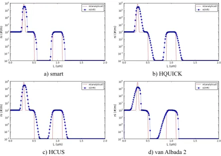
4.1.4 Stiff nucleation at a negligible size
In this problem, the performance of high resolution schemes for a batch process with stiff nucleation and constant growth rate is analysed. It was assumed that the nucleation takes place at the minimum size L0 = 0 with the nucleation rate given by:
(34)
The growth rate is 1μm/s and the crystal size distribution is given in the size range of [0, 2]μm discretised into 200 elements. The analytical solution for this case is:
(35) The initial number density function is given by:
The first region in the solution is a narrow wave originating from the nucleation while the second region is a square step with a sharp discontinuity. The results are compared to the analytical solution: the best three high-resolution schemes (a-c) and the worst one (d) are presented in Fig. 9. L1 and L2 norms for high-resolution schemes are given in Table 5.
Similarly to the case study in the section 4.1.2, discretisation schemes have problems with the very sharp peaks in the size distribution. Again, all high-resolution schemes performed approximately equally well with a significant degree of numerical diffusion present in all schemes. Overall, smart, HQUICK and HCUS flux limiters showed somewhat better prediction than the rest.
Based on the numerical problems in sections 4.1.1 to 4.1.4 an overall conclusion is that superbee and Koren flux limiter showed better results in most of the cases considered and that all schemes produce a significant numerical diffusion when sharp peak-like fronts are present in the distribution. Therefore, in a general case, selection of a suitable flux limiter function is case-dependent and some experimenting is necessary.
4.2 Growth-only cooling crystallisation (hydrodynamics effects)
In this case study, the effect of hydrodynamics in a poorly mixed reactor were analysed. The growth only cooling crystallization problem has been used, since the analytical solution can be easily obtained while the effect of the other phenomena is absent. The results from four different cases were compared: a) ideal mixing assumed and crystallization modelled using the discretised population balance (IDMIX+DPB), b) ideal mixing assumed and crystallization modelled using the method of characteristics (IDMIX+MOCH), c) SPH used for fluid dynamics coupled with the discretised population balance model, applied to every fluid particle (SPH+DPB), and d) SPH coupled with the method of characteristics, again applied to every fluid particle (SPH+MOCH). A low rpm of the stirrer and short impeller blades were used to create poor mixing conditions. The temperature profile in both ideal mixing cases was set to the calculated average temperature profile of the SPH cases to create the identical cooling conditions. The domain was discretized using 200 elements. The process studied was crystallisation of paracetamol from ethanol solution in the 1 lit Labmax reactor using the kinetic data from Mitchell et al. (2011a). The initial supersaturation ratio was set to 1.5667, the initial temperature to 200C,
temperature was constant and equal to 00C. The stirred tank wall, baffles and stirrer surface
meshes are presented in the Fig. 10. The stirred tank filled with fluid particles of the radius 1.5mm is given in Fig. 11. The ideal mixing models coupled with DPB/MOCH methods were developed in Python using DAE Tools software (Nikolic, 2014). The model equations are identical to the model equations presented in (Mitchell et al., 2011a). The only difference is that the method of moments equations were replaced by the DPB or MOCH equations and that the temperature profile in the ideal mixing case was set to the calculated average temperature of the SPH cases.
(yellow) and have approximately uniform growth rate. Next, the mostly static particles along the wall in the zone 2 (blue) have a high cooling rate and a faster growth and form the front end of the CSD. Finally, the particles that belong to the poorly mixed zone 3 (red) away from the walls, have a low cooling rate and therefore a lower growth rate and form the CSD tail.
4.3 Cooling crystallisation with primary nucleation (SPH+DPB vs SPH+MOCH)
In this case study, the capability of SPH+DPB and SPH+MOCH methods to handle sharp fronts/peaks in the distribution occurring during the primary nucleation was studied. The process was cooling crystallization starting with primary nucleation followed by growth. All runtime parameters and kinetics data are identical to those in the previous problem (section 4.2). The equation for the primary nucleation kinetics is adopted from the work of Mitchell et al. (2011b):
(37)
with kn = 1.597 x 10¹⁰ #/(min x m3)n and n = 2.276. The initial CSD is assumed to be empty
and the models were again simulated for 300s. The simulation results are shown in Fig. 16. As it was previously discussed in the section 4.1 the DPB method is not able to accurately track sharp peak-like discontinuities in the solution and a significant degree of numerical diffusion is present in those cases. On the other hand, the MOCH method produces the results identical to the analytical solution.
4.4 Benchmarking and computational requirements
algorithm, analyse the data in terms of the computational requirements, detect the bottlenecks and propose the most efficient method from the computational perspective. The results are presented in Tables 6 to 9, while a graphical comparison for 300 bins is given in Fig. 17. The data represent durations in milliseconds of individual stages in the algorithm for a single time step during the simulation. Three main stages were considered: calculation
of forces for Navier-Stokes equations and gradients for heat/mass transfers (stage: N-S
forces), integration of Navier-Stokes equations and heat/mass balances (stage: N-S integration), integration of population balance equations (stage: PB integration). OpenMP
methods contain two additional stages: waiting on OpenMP barriers (stages: OpenMP
barrier 1 and 2) and data synchronisation between GPU and main memory (stage: Memory copy). All results are averaged over approximately two thousand time steps.
data to be fetched from the main memory). For instance, the overhead due to the time spent on barriers and memory synchronisation in the case with 200 bins is significant: 21% in SPH+DPB+OpenMP and 17% in SPH+MOCH+OpenMP case. The other contributing factor is longer calculation of forces and longer integration of Navier-Stokes equations since the data structure in memory holding the particle information is larger and an additional time is required to fetch larger chunks of memory.
The advantage of application of the SPH method to modelling of the integrated fluid dynamics and crystallisation process is that a very large number of bins or characteristic lines can be used. For instance, the SPH+MOCH+OpenMP simulation with 500 characteristic lines is only 18% slower compared to 200 characteristic lines. Obviously, there is a lot of room for further optimisations: use of more processors, multiple GPUs, and merging the memory copy routine with the population balance integration stage. The above-mentioned optimisations will be a part of the future work.
5. Conclusions
The integrated SPH and population balance model has been developed based on the fluid dynamics model presented in Nikolic and Frawley (2015). Two existing methods for solution of population balance equations have been implemented: a) discretised population balance method solved using the high-resolution finite volume schemes with flux limiter, and b) method of characteristics. Both methods have successfully been applied to numerical benchmarking problems available in the literature where the analytical solutions are available. The algorithm to integrate the population balance equations in parallel and independently from the Navier-Stokes equations has been developed. It has been shown that the population balance equations can be solved using the OpenMP interface while the fluid dynamics equations being computed independently on a GPGPU using the NVidia CUDA technology. The benefits of the proposed methodology were pointed out such as significantly lower computational requirements and availability of the crystal size distribution. This way, a significant portion of the computational overhead due to a large number of additional transport equations resulting from the discretisation of the population balance can be removed: the total overhead was reduced to only 40% for 200 additional equations, compared to CFD-only simulation.
of characteristics has been selected as computationally more efficient and more accurate for problems where sharp or peak-like gradients are present in the distribution.
Acknowledgments:This research has been conducted as part of the Synthesis and Solid State Pharmaceutical Centre (SSPC) and funded by Science Foundation Ireland (SFI).
Nomenclature
B – birth rate, #/(m.m3.s) C – concentration, mol/m3
ΔC – supersaturation, mol/m3 D – diffusivity coefficient, m/s
cp – heat capacity, J/(kg.K)
ri-rj – distance between two particles, m
g – gravity constant, m/s
G – growth rate, m/s
h – smoothing length, m
L – crystal size or size discretization domain, m
m – mass od the particle, kg
n, ni – number density function, #/(m.m3) p – pressure, Pa
p0 – pressure magnitude for the equation of state, Pa
r – position of a particle in space (x,y,z), m
s – source term in the population balance equation (births - deaths), #/(m.m3.s)
S – source term integral,
T – temperature, K
u – velocity, m/s
z – parameter representing the measure of the distance along the characteristic line,
-W – Smoothing kernel, - Greek symbols
λ – thermal conductivity, W/(m.K) μ – viscosity, Pa.s
ρ – density, kg/m3
References
Aamir E, Nagy ZK, Rielly CD, Kleinert T, Judat B. Combined quadrature method of moments and method of characteristics approach for efficient solution of population balance models for dynamic modelling and crystal size distribution control of crystallization processes. Ind. Eng. Chem. Res. 2009;48:8575–8584.
doi:10.1021/ie900430t.
Alopaeus V, Laakkonen M, Aittamaa J. Numerical solution of moment-transformed
population balance equation with fixed quadrature points. Chem. Eng. Sci. 2006;61: 4919-4929. doi:10.1016/j.ces.2006.03.028.
Chakravarthy SR, Osher S. High resolution applications of the Osher upwind scheme for the Euler equations. Proc. AIAA 6th Computational Fluid Dynamics Conference 1983;363–373. AIAA Paper 83-1943.
Costa CBB, Maciel MRW, Filho RM. Considerations on the crystallization modeling: population balance solution. Comp. Chem. Eng. 2007;31:206–218.
doi:10.1016/j.compchemeng.2006.06.005.
Fan R, Marchisio DL, Fox RO. Application of the direct quadrature method of moments to polydisperse gas-solid fluidized beds. Powder Technol. 2004;139:7-20.
doi:10.1016/j.powtec.2003.10.005
Gaskell PH, Lau AKC. Curvature-compensated convective transport: SMART, a new boundedness-preserving transport algorithm. Int. J. Num. Meth. Fluids 1988;8:617– 641. doi:10.1002/fld.1650080602.
Gunawan R, Fusman I, Braatz RD. High Resolution Algorithms for Multidimensional Population Balance Equations. AIChE J. 2004;50:11. doi:0.1002/aic.10228. Haseltine EL, Rawlings JB. On the origins of approximations for stochastic chemical
kinetics. J. Chem. Phys. 2005;123:164115. doi:10.1063/1.2062048.
Hounslow MJ, Reynolds GK. Product engineering for crystal size distribution. AIChE J. 2006;52:2507. doi:10.1002/aic.10874.
John V, Angelov I, Öncül AA, Thévenin D. Towards the optimal reconstruction of a distribution from its moments. Chem. Engi. Sci. 2007;62:2890-2904.
Kermani MJ, Gerber AG, Stockie JM. Thermodynamically Based Moisture Prediction Using Roe’s Scheme. 4th Conference of Iranian AeroSpace Society, Amir Kabir University of Technology, Tehran, Iran, January 27–29 2003.
Koren B. A robust upwind discretisation method for advection, diffusion and source terms. In: Vreugdenhil CB, Koren B, editors. Numerical Methods for Advection–Diffusion Problems. Braunschweig: Vieweg; 1993. ISBN-3-528-07645-3.
Kumar S, Ramkrishna D. On the solution of population balance equations by discretization - I. A fixed pivot technique. Chem. Eng. Sci. 1996a;51:1311-1332.
Kumar S, Ramkrishna D. On the solution of population balance equations by discretization - II. A moving pivot technique. Chem. Eng. Sci. 1996b;51:1333-1342.
LeVeque RJ. Finite Volume Methods for Hyperbolic Problems. Cambridge University Press, UK; 2002. ISBN-13: 978-0521009249.
Lien FS, Leschziner MA. Upstream monotonic interpolation for scalar transport with application to complex turbulent flows. Int. J. Num. Meth. Fluids 1994;19:527–548. doi:10.1002/fld.1650190606.
MacDonald A. Fluidix v1.0.3. OneZero Software, http://www.onezero.ca; 2014. Marchisio DL, Ptkturna JT, Vigil RD, Fox RO. Quadrature method of moments for
population balance equations. AIChE J. 2003;49:1266. doi:10.1002/aic.690490517. McGraw R. (1997), Description of aerosol dynamics by the quadrature method of
quadrature method of moments. J. Aerosol Sci. 2003;34:189–209. doi:10.1016/S0021-8502(02)00157-X.
Mitchell NA, Ó’Ciardhá CT, Frawley PJ. Estimation of the growth kinetics for the cooling crystallisation of paracetamol and ethanol solutions. J. Cryst. Growth 2011a;328:39-49. doi:10.1016/j.jcrysgro.2011.06.016.
Mitchell NA, Frawley PJ, Ó’Ciardhá CT. Nucleation kinetics of paracetamol–ethanol solutions from induction time experiments using Lasentec FBRM®. J. Cryst. Growth 2011b;321:91–99. doi:10.1016/j.jcrysgro.2011.02.027.
Monaghan JJ, Huppert HE, Worster MG. Solidification using smoothed particle
hydrodynamics. J. Comp. Phys. 2005;206:684–705. doi:10.1016/j.jcp.2004.11.039. Nigam KM, Nigam KDP. Application of Galerkin technique to diffusion problems in
tubular reactor. Chem. Eng. Sci. 1980;35:2358−2360. Nikolic DD. DAE Tools v1.4.0, http://www.daetools.com; 2014.
Nikolic DD, Frawley PJ. Application of the Lagrangian Meshfree Approach to Modelling of Batch Crystallisation: Part I – Modelling of Stirred Tank Hydrodynamics, Chem. Eng. Sci., Available online 28 September 2015, doi:10.1016/j.ces.2015.08.052. Qamar S, Elsner MP, Angelov IA, Warnecke G, Seidel-Morgenstern A. A comparative study
of high resolution schemes for solving population balances in crystallization. Comp. Chem. Eng. 2006;30:1119-1131. doi:10.1016/j.compchemeng .2006.02.012.
Ramkrishna D. Population Balances: Theory and Applications to Particulate Systems in Engineering. Academic Press, New York; 2000. ISBN-13: 060-8628697093. Randolph AD, Larson MA. Theory of particulate processes. Analysis and techniques of
continuous Crystallization. Academic Press, San Diego, CA, USA; 1971. Roe PL. Characteristic-based schemes for the Euler equations. Ann. Rev. Fluid Mech.
1986;18:337–365. doi:10.1146/annurev.fl.18.010186.002005.
Rosner DE, McGraw R, Tandon P. Multivariate Population Balances via Moment and Monte Carlo Simulation Methods: An Important Sol Reaction Engineering Bivariate Example and “Mixed” Moments for the Estimation of Deposition, Scavenging, and Optical Properties for Populations of Nonspherical Suspended Particles. Ind. Eng. Chem. Res. 2003;42:2699-2711. doi:10.1021/ie020627l. Roussos AI, Alexopoulos AH, Kiparissides C. Part III: Dynamic evolution of the particle
size distribution in batch and continuous particulate processes: A Galerkin on finite elements approach. Chem. Eng. Sci. 2005;60:6998−7010.
Singh PN, Ramkrishna D. Solution of population balance equations by MWR. Comp. Chem. Eng. 1977;1:23-31. doi:10.1016/0098-1354(77)80004-5.
Sporleder F, Dorao CA, Jakobsen HA. Model based on population balance for the
simulation of bubble columns using methods of the least-squares type. Chem. Eng. Sci. 2011;66:3133−3144.
Sweby PK. High resolution schemes using flux-limiters for hyperbolic conservation laws. SIAM J. Num. Anal. 1984;21:995–1011. doi:10.1137/0721062.
Van Albada GD, Van Leer B, Roberts WW. A comparative study of computational methods in cosmic gas dynamics. Astronomy and Astrophysics 1982;108:76-84.
Van den Bosch B, Padmanabhan L. Use of orthogonal collocation methods for the
modeling of catalyst particles-I. Analysis of the multiplicity of the solutions. Chem. Eng. Sci. 1974;29:1217−1225.
Van Leer B. Towards the ultimate conservative difference scheme II. Monotonicity and conservation combined in a second order scheme. J. Comp. Phys. 1974;14:361–370. doi:10.1016/0021-9991(74)90019-9.
Van Leer B. Upwind-difference methods for aerodynamic problems governed by Euler equations. Lectures in applied mathematics, part 2: Vol. 22, Providence, RI: American mathematical Society; 1985.
Waterson NP, Deconinck H. A unified approach to the design and application of bounded higher-order convection schemes, VKI Preprint; 1995.
Tables
Table 1. Flux limiters
Flux limiter Formula
CHARM (Zhou, 1995)
HCUS (Waterson and Deconinck, 1995)
HQUICK (Waterson and Deconinck, 1995)
Koren (Koren, 1993) MC (van Leer, 1977) minmod (Roe, 1986)
Osher (Chakravarthy and Osher, 1983)
ospre (Waterson and Deconinck, 1995)
smart (Gaskell and Lau, 1988) superbee (Roe, 1986)
Sweby (Sweby, 1984)
UMIST (Lien and Leschziner, 1994)
vanAlbada1 (van Albada et al., 1982)
vanAlbada2 (Kermani et al., 2003)
vanLeer (van Leer, 1974)
Table 2. Performance of flux limiters for the size-independent growth I case (L2 sorted)
Flux limiter ||n||1 ||n||2
superbee 1.827e+10 0.716e+10
Sweby 2.678e+10 0.857e+10
Koren 3.496e+10 1.025e+10
smart 3.562e+10 1.039e+10
HCUS 4.167e+10 1.083e+10
MC 3.966e+10 1.100e+10
HQUICK 4.213e+10 1.101e+10
vanLeer-minmod 4.128e+10 1.113e+10
CHARM 4.424e+10 1.116e+10
vanLeer 4.562e+10 1.165e+10
ospre 4.757e+10 1.180e+10
vanAlbada1 5.126e+10 1.203e+10
Osher 5.303e+10 1.231e+10
UMIST 5.356e+10 1.255e+10
minmod 6.744e+10 1.356e+10
vanAlbada2 6.415e+10 1.405e+10
Table 3. Performance of flux limiters for the size-independent growth II case (L2 sorted)
Flux limiter ||n||1 ||n||2
superbee 4.464e+10 1.015e+10
smart 4.727e+10 1.120e+10
Koren 4.861e+10 1.141e+10
MC 5.129e+10 1.162e+10
Sweby 5.435e+10 1.142e+10
HCUS 5.528e+10 1.194e+10
HQUICK 5.531e+10 1.194e+10
vanLeer-minmod 5.600e+10 1.202e+10
vanLeer 5.814e+10 1.225e+10
ospre 6.131e+10 1.252e+10
UMIST 6.181e+10 1.259e+10
vanAlbada1 6.600e+10 1.281e+10
Osher 6.690e+10 1.275e+10
minmod 7.751e+10 1.360e+10
Table 4. Performance of flux limiters for the size-dependent growth case (L2 sorted)
Flux limiter ||n||1 ||n||2
vanAlbada2 12.0030 6.08332
ospre 12.0030 7.53221
vanAlbada1 12.0030 8.79521
Koren 12.0030 9.67953
smart 12.0030 9.68046
UMIST 12.0030 9.68063
vanLeer 12.0030 9.68106
HCUS 12.0030 9.68543
vanLeer-minmod 12.0030 9.68618
MC 12.2824 9.69038
HQUICK 12.0030 9.69071
Sweby 12.0030 9.69257
Osher 12.0372 9.71215
minmod 12.0372 9.71218
superbee 13.3472 9.75628
Table 5. Performance of flux limiters for the stiff nucleation at negligible size case (L2
sorted)
Flux limiter ||n||1 ||n||2
smart 2.08484e+06 8.29318e+05
HQUICK 2.18136e+06 8.42675e+05
HCUS 2.19180e+06 8.50234e+05
Koren 2.14188e+06 8.51961e+05
Sweby 2.16105e+06 8.53665e+05
superbee 2.04586e+06 8.56988e+05
vanLeer-minmod 2.19952e+06 8.60628e+05
MC 2.16293e+06 8.60771e+05
vanLeer 2.22526e+06 8.66659e+05
Osher 2.27713e+06 8.67580e+05
ospre 2.06679e+06 8.68821e+05
UMIST 2.25735e+06 8.72690e+05
vanAlbada1 2.21372e+06 8.76436e+05
minmod 2.35476e+06 8.92151e+05
Table 6. Profiling of SPH+DPB simulations (Nparticles = 37038, Rp =1.50 mm) Stage SPH-only Duration in [ms] for different number of bins
200 300 400 500 1000
N-S forces 13.468 15.706 15.772 15.786 15.817 15.836
N-S integration 6.320 6.567 6.493 6.537 6.518 6.529
PB integration 15.590 22.457 31.680 39.898 79.841
Total time step 19.784 37.860 44.717 53.999 62.228 102.201
Slowdown (to SPH-only): 91% 126% 173% 215% 417%
Table 7. Profiling of SPH+MOCH simulations (Nparticles = 37038, Rp =1.50 mm) Stage SPH-only Duration in [ms] for different number of bins
200 300 400 500 1000
N-S forces 13.468 15.730 15.857 15.595 15.731 16.953
N-S integration 6.320 6.606 6.627 6.465 6.553 6.550
PB integration 6.302 10.617 12.637 15.497 27.858
Total time step 19.784 28.657 33.096 34.694 37.777 51.356
Slowdown (to SPH-only): 45% 67% 75% 91% 160%
Table 8. Profiling of SPH+DPB+OpenMP simulations (Nparticles = 37038, Rp =1.50 mm)
Stage SPH-only Duration in [ms] for different number of bins
200 300 400 500 1000
N-S forces 13.468 15.700 16.040 18.166 18.555 18.605
N-S integration 6.320 8.913 9.318 9.578 9.500 9.438
Memory copy 2.784 2.999 3.125 3.146 3.649
OpenMP barrier 1 0.888 7.526 12.483 18.749 53.675
OpenMP barrier 2 0.484 0.442 0.433 0.428 0.452
PB integration 16.689 24.004 30.687 37.692 71.538
Total time step 19.784 28.787 36.364 43.820 50.414 85.851
Slowdown (to SPH-only): 46% 84% 121% 155% 334%
Table 9. Profiling of SPH+MOCH+OpenMP simulations (Nparticles = 37038, Rp =1.50
mm)
Stage SPH-only Duration in [ms] for different number of bins
200 300 400 500 1000
N-S forces 13.468 15.179 15.209 15.198 15.237 18.202
N-S integration 6.320 9.662 11.182 12.900 14.389 18.115
Memory copy 2.466 2.902 2.533 2.689 3.031
OpenMP barrier 1 0.468 0.457 0.437 0.423 0.441
OpenMP barrier 2 0.355 0.410 0.385 0.413 0.428
PB integration 5.200 7.939 10.623 13.304 26.758
Total time step 19.784 28.170 30.257 31.501 33.224 40.251
Figures
Figure 1. Cell-centered finite volume discretisation
Figure 4. Size-independent growth I at time t = 60s (I-order upwind and II-order central schemes)
a) superbee b) Sweeby
c) Koren d) van Albada 2
a) superbee b) Smart
c) Koren d) van Albada 2
a) van Albada 2 b) ospre
c) van Albada 1 d) superbee
a) van Albada 2 b) ospre
c) van Albada 1 d) superbee
a) smart b) HQUICK
c) HCUS d) van Albada 2
Figure 10. LabMax stirred tank surface meshes: reactor wall (dark green), baffles (yellow) and Rushton turbine (light green)
Figure 12. Temperature of the particles in the axial cross section of the reactor for the
a) Ideal mixing
b) SPH
a) Ideal mixing
b) SPH
Figure 16. Simulation results for cooling crystallisation with primary nucleation at t = 300s
Figure 17. Profiling data (Nparticles = 37038, Rp =1.50 mm, 300 bins)
© 2016 by the authors; licensee Preprints, Basel, Switzerland. This article is an open access article distributed under the terms and conditions of the Creative Commons by