DOI10.1186/2190-8567-3-4
R E S E A R C H Open Access
A Network Model of the Periodic Synchronization
Process in the Dynamics of Calcium Concentration
in GnRH Neurons
Maciej Krupa·Alexandre Vidal· Frédérique Clément
Received: 1 November 2012 / Accepted: 22 March 2013 / Published online: 10 April 2013
© 2013 M. Krupa et al.; licensee Springer. This is an Open Access article distributed under the terms of the Creative Commons Attribution License (http://creativecommons.org/licenses/by/2.0), which permits unrestricted use, distribution, and reproduction in any medium, provided the original work is properly cited.
Abstract Mathematical neuroendocrinology is a branch of mathematical neuro-sciences that is specifically interested in endocrine neurons, which have the uncom-mon ability of secreting neurohoruncom-mones into the blood. One of the most striking features of neuroendocrine networks is their ability to exhibit very slow rhythms of neurosecretion, on the order of one or several hours. A prototypical instance is that of the pulsatile secretion pattern of GnRH (gonadotropin releasing hormone), the master hormone controlling the reproductive function, whose origin remains a puzzle issue since its discovery in the seventies. In this paper, we investigate the question of GnRH neuron synchronization on a mesoscopic scale, and study how synchronized events in calcium dynamics can arise from the average electric activity of individual neurons. We use as reference seminal experiments performed on embryonic GnRH neurons from rhesus monkeys, where calcium imaging series were recorded simultaneously in tens of neurons, and which have clearly shown the occurrence of synchronized calcium peaks associated with GnRH pulses, superposed on asynchronous, yet oscil-latory individual background dynamics. We design a network model by coupling 3D individual dynamics of FitzHugh–Nagumo type. Using phase-plane analysis, we con-strain the model behavior so that it meets qualitative and quantitative specifications derived from the experiments, including the precise control of the frequency of the
M. Krupa·F. Clément
Project-Team SISYPHE, INRIA Paris-Rocquencourt Research Centre, Domaine de Voluceau, Rocquencourt BP 105, 78153 Le Chesnay cedex, France
M. Krupa
e-mail:[email protected]
F. Clément
e-mail:[email protected]
A. Vidal (
)Laboratoire Analyse et Probabilités, IBGBI, Université d’Évry-Val-d’Essonne, 23 boulevard de France, 91037 Evry cedex, France
synchronization episodes. In particular, we show how the time scales of the model can be tuned to fit the individual and synchronized time scales of the experiments. Finally, we illustrate the ability of the model to reproduce additional experimental observations, such as partial recruitment of cells within the synchronization process or the occurrence of doublets of synchronization.
Keywords Mathematical neuroendocrinology·GnRH neurons·Calcium dynamics·Multiple time scale dynamics·Mixed-mode oscillations (MMOs)· Network model·Synchronization/desynchronization·Pulsatile rhythm·Frequency control
List of Abbreviations
GnRH: Gonadotropin Releasing Hormone IPI: InterPeak Interval
MMOs: Mixed-Mode Oscillations
1 Introduction
GnRH (gonadotropin releasing hormone) plays a prominent role in the control of reproductive processes in mammals. GnRH is a neurohormone released into the pi-tuitary portal blood by hypothalamic GnRH neurons in a pulsatile manner. The pul-satile nature of this release is important for the proper functioning of the reproduc-tive system. To date, the mechanisms behind the pulsatility are poorly understood as GnRH neurons present a significant challenge to experimental studies. They are scarce, sparsely located in the hypothalamus and interspersed with other neuronal and glial cells.
However, although GnRH neurons are sparsely located in the hypothalamus, they all have an extracerebral origin in the nasal (olfactory) placode, where they develop and from where they migrate to the brain during the development of the embryo. This feature was used in a number of studies in different species (rodents, primates, sheep) [1,2]. In particular, Terasawa et al. [3] studied cultures of pre-GnRH neurons obtained from fetuses of rhesus monkeys. It is an accepted view in the community working on placode cultures that the neurons develop in the culture in a similar way as they would in vivo [4]. Terasawa et al. [3,5] made a series of experiments, measur-ing GnRH release, calcium levels, and the electric activity in the cultured embryonic GnRH neurons. Remarkably, as reported in [4], placode GnRH neurons are able to release GnRH in a pulsatile manner and at frequency very close to that observed in vivo in adult animals and this process is calcium dependent. Detailed investigations of calcium dynamics revealed that calcium levels evolved in an oscillatory manner in each cell, mostly independent from cell to cell, with the exception of periodically occurring episodes of synchronization. The oscillations in the individual neurons oc-curred on the scale of approximately 10 min and the synchronization events roughly with the period of one hour. During the synchronization events the maximal calcium levels were typically much higher than during the independent oscillations.
expressing Green Fluorescent Protein (GFP) specifically in GnRH neurons [7]. These studies provide evidence of the presence of three modes of oscillation, with the two slower modes possibly related to the individual and synchronized calcium oscilla-tions. Together with the findings of [3] this led to the following working hypothesis: The peaks of the intermediate oscillation of the electric activity coincide with the in-dividual calcium peaks, whereas the peaks of the slowest oscillation of the electric activity coincide with the synchronized calcium peaks. Finally, since the excitation-secretion coupling mediated by calcium is well documented in other types of cells (see the discussion in [4]), we suggest the following causal sequence: increased elec-tric activity−→synchronized calcium peaks−→pulse of GnRH release.
In this article, we propose a phenomenological model that can produce patterns of oscillations consistent with the experimental results described above. On a more generic ground, our model provides a mathematical mechanism of the genesis of synchronized events superimposed on faster, individual oscillations. We introduce a three-dimensional model based on the FitzHugh–Nagumo system that reproduces the average electric activity and the intracellular calcium oscillations in individual neu-rons. This model has a mathematical structure that makes it possible to explain, study and control the dynamics by means of phase plane analysis. Moreover, the model can generate calcium patterns fulfilling qualitative and quantitative specifications: peak heights, baseline level, InterPeak Interval (IPI). We build the network model by introducing a network level (global) variable that mediates periodic fluctuation of ex-citability of the neurons, whose increase leads to episodes of electric synchronization and to calcium peaks. We show by a combination of analysis and simulations that our model can, in a robust manner, reproduce the alternation of asynchronous phases, episodes of calcium peak synchronization and postexcitatory suppression. We prove, in particular, how the time scales can be adjusted so that they agree with the individ-ual and synchronized time scales of the experiment reported on in [3]. We also show the ability of the model to reproduce additional experimental observations, such as partial recruitment of the cells within the synchronization process and the occurrence of doublets of synchronization.
Synchronization of coupled oscillators has been widely studied, and the ideas de-veloped in our paper have their origin in some of these earlier works. Many studies have focused on the setting of weakly coupled oscillators, in physics; see [8] for a review, in mathematics [9,10], and in neuroscience [11]. In its simplest form, the context of such studies have been networks of coupled phase oscillators [12,13]. More general models can be reduced to coupled phase oscillators; in this reduction, the asymptotic phase of the individual oscillators, or equivalently, the foliation by isochrones, is used to derive the so-called Phase Resetting Curve, which gives rise to the coupling function [10,11]. Synchronization depends on the structure of the cou-pling; some of the frequently considered coupling architectures are “nearest neigh-bor” [10], “all-to-all” [13], and global coupling, that is coupling that depends on a global variable, e.g., the average of the phases. Examples of systems with global cou-pling are coupled arrays of Josephson junctions [14] and a model of the Belousov– Zhabotinsky reaction with global feedback [15].
see, for example, [16]. Our model is inspired by the work of [16], who considered the so-called PING model of gamma oscillations, consisting of a population of excitatory cells and a population of interneurons, with the interneurons delivering inhibition simultaneously to all excitatory cells, thus creating a synchronizing effect. We have adapted this idea to the context of our model, creating a global variable which would have a similar, strong effect on all the members of the population, giving rise to a synchronous calcium peak.
This article is organized as follows. In Sect.2, we review the results of [3] and [5] in more detail, preparing the ground for the construction, analysis, and simulation of our model. In Sect.3, we introduce and analyze the individual cell model. We addi-tionally show how to reproduce the variability in the IPI and peak height by varying two specific parameters. In Sect.4, we consider the coupled dynamics of a population of GnRH neurons, introduce the network model, and explain the dynamical mecha-nisms that underlie the emergence of the desired oscillation patterns. In particular, we show how to control the frequency of the synchronization episodes, and obtain a rigorous estimate for the simplest case. In Sect.5, we present numerical simulations that reproduce the periodic sequence of synchronization, postexcitatory suppression and desynchronization phases. We show how to mimic partial recruitment of the cells in the synchronization episodes and how to reproduce synchronization doublets.
2 Intracellular Calcium Patterns in Embryonic GnRH Neurons
In this section, drawing mostly on the results of [3] and [5], we review the main qualitative and quantitative properties of intracellular calcium patterns in cultured embryonic GnRH cells.
Calcium data in [3] and [5] were obtained by means of calcium imaging: cells were loaded with fluorochrome (fura 2) and exposed to light excitation at specific UV wavelengths. As the dye’s fluorescence properties are altered when it is bound to calcium, its relative light emission in response to different wavelengths can be used to estimate intracellular calcium concentration [17]. The data were acquired every 5 to 10 seconds during up to 170 minute periods.
Figure 5 in [3] (http://www.jneurosci.org/content/19/14/5898/F5.expansion.html) shows, on the same graph, the pattern of intracellular calcium in 50 embryonic GnRH cells during 152 minutes as well as zooms of this graph over three different time intervals of 18 minute length. Each calcium pattern fits the type described above and displayed in Fig. 1 in [3]. Most of the time, the calcium patterns are independent among cells (unsynchronized, with different IPI and peak levels).
The most striking result of [3], sometimes referred to as the Terasawa puzzle, is the existence of isolated episodes of synchronization: Almost all cells begin a peak at approximately the same time and for each cell recruited in the synchronization the height of its calcium peaks during a synchronized peak is higher than the peak heights attained outside of the synchronization periods (see Fig. 5 in [3], where three synchronized peaks are shown). These episodes of synchronization are followed by a “postexcitatory suppression” of a few minutes during which calcium levels are at the baseline in all cells. Moreover, the episodes of synchronization occur at regular intervals of nearly 60 minutes (between 59 and 61 minutes). There is also a gradual decrease in the signal amplitude (due to photobleaching) inherent in the experimental protocol and that we do not intend to capture with our modeling study.
3 A Model of Intracellular Calcium Dynamics in Single GnRH Neuron
We use the excitability property of the FitzHugh–Nagumo dynamics to generate pe-riodic oscillations of Ca that fit the qualitative pattern obtained in [3] and described in the preceding section. Moreover, the FitzHugh–Nagumo dynamics is well under-stood, which allows us to control the quantitative properties of the oscillatory events. We consider the following model for one neuron:
x=τ−y+4x−x3−φfall(Ca)
, (1a)
y=τ εk(x+a1y+a2), (1b)
Ca=τ ε
φrise(x)−
Ca−Cabas
τCa
, (1c)
with
φfall(Ca)=
μCa Ca+Ca0
,
φrise(x)=
λ
1+exp(−ρCa(x−xon))
.
(2)
Whenφriseis inactive (φrise(x)close to 0), Ca decreases to a quasi steady state close
to Cabas which represents the baseline of the intracellular calcium level. The speed
of this motion is determined by theτ ε/τCaratio (exponential decay rate). Ca acts as
a feedback onto thex dynamics through the increasing functionφfall(Ca)bounded
byμ. The effect of this coupling is to reduce the electric activity of the neuronal population in response to the rise of the calcium concentration. An analogous term is used in models of single neurons to represent the hyperpolarization of the cell mem-brane stimulated by calcium; see [19] for an example. We explain in the following how, in a certain range of parameter values, the cell may stay in the “hyperpolarized regime” ((x, y)to the left of the lower knee of the fast nullcline) while the values of the calcium concentration remain low.
The values of parameterai are chosen according to the well-known properties of the FitzHugh–Nagumo oscillators. Hence, we take a classic cubic dynamics for the
xdynamics. By default, we setk=1 and we assumea1to be negative and small, so
that they nullcline is steep. In the following, we seta1= −0.1, which ensures that
thexandy nullclines intersect only at one point. Parametersμand Ca0are positive,
ensuring thatφfall(Ca)is well-defined and positive for all positive values of Ca.
3.1 Qualitative Study of the Single GnRH Neuron Model
Depending on the value of Ca considered as a parameter, the slow–fast FitzHugh– Nagumo oscillator (1a)–(1b) can be in an oscillatory, excitable or steady regime:
1. Oscillatory regime: they nullcline intersects the cubicx nullcline on its middle branch (between the two knees). This singular point is unstable and the system displays a globally attractive limit cycle of relaxation type.
2. Excitable regime: the singular point lies on either the left or the right branch close to the knee. The excitability of the system is then characterized by the following property. Let us consider the stable singular point lying on the left branch of the cubic near the left knee as initial condition. Then a small perturbation of this initial condition introduced by increasingxand/or decreasingyimplies a large excursion of the orbit near the right branch of the cubic toward the right knee and back to the vicinity of the left branch before asymptotically reaching the singular point. 3. Steady regime: the singular point lies on either the left or the right branch far away
from the knees: the singular point is then stable and attracts any orbit of (1a)–(1b). The perturbation from the steady state has to be large enough to bring about a large excursion in the phase portrait.
Let us recall that the transition between the excitable state and the oscillatory regime that occurs in a very narrow interval of Ca values is the well-known canard phe-nomenon, leading to the existence of small attractive limit cycle following the middle branch of the cubic for a while [20]. When considering the 3D model, the periodic exploration of the regions corresponding to oscillatory regime and excitable regime of subsystem (1a)–(1b) may produce mixed-mode oscillations (MMOs). We will use this feature to reproduce the quiescent phase in the generated Ca pattern.
this work, we will take advantage of the fact that MMO dynamics can reproduce the features of the individual calcium oscillations and that the passage between different types of MMOs can be easily controlled, especially in systems where MMOs arise via the mechanism of slow passage through a canard explosion [22,23].
System (1a)–(1c) is a slow–fast system with one fast and two slow variables. To describe the dynamical mechanisms underlying the behavior of the system, we intro-duce the following notations. The critical manifoldS0(orxnullcline), given by
y=4x−x3−φfall(Ca), (3)
is an S-shaped surface embedding two fold linesF−, contained in the half-space
x <0, andF+, contained in the half-spacex >0. The fold lines splitS0into three parts (see Fig.1): the left and right sheets contained entirely in the half-spacesx <0 andx >0, respectively, and a middle sheet. Theynullcline, defined by
a0x+a1y+a2=0, (4)
is a plane that crossesF−for a given value Caf of Ca. The Ca nullcline is an attrac-tive surface for the Ca dynamics and is defined by
Ca=τCaφrise(x)+Cabas. (5)
The right-hand side of (5) is, likeφrise, a smooth sigmoidal function ofx.
We now describe the typical interactions between the state variables, starting from a low level of Ca (i.e., close to Cabas) and a pair(x, y)such that(x, y,Ca)lies just
below F−. Under the influence of the fast dynamics, the current point(x, y,Ca)
quickly reaches the right sheet of S0, so that x and τCaφrise(x)quickly increase.
Consequently, Ca increases while the current point moves up along the right sheet of
S0towardF+. Then, once the current point has arrived aboveF+, it quickly comes back near the left sheet ofS0 under the influence of the fast dynamics; variablex
quickly decreases as well as the termτCaφrise(x)(which becomes almost zero). The
current point, driven by the slow dynamics, moves down along the left sheet ofS0and Ca decreases eventually down to Cabas. Then several situations may occur depending
mainly on the value ofμand related to the regime of system (1a)–(1b):
A: For small values ofμ, when the current point reaches the vicinity ofF−, system (1a)–(1b) is in the oscillatory regime. As a consequence, the current point directly and quickly reaches the right sheet ofS0, and the behavior described above re-peats immediately. An example of such an orbit is represented in panel (a) of Fig.1.
B: For an interval of values ofμ, system (1a)–(1b) is in the excitable regime when Ca approaches Cabas. Then (x, y)reaches the vicinity of the singular point of
Fig. 1 Different types of system (1a)–(1c) orbits according to the value ofμ. In eachpanel, thecyan surfacerepresents thexnullclineS0whose foldsF±are represented byred lines.aAttractive periodic orbit without small oscillations near the foldF−. This type of orbit is obtained for small values ofμ.
bAttractive MMO limit cycle with small oscillations near the foldF−. This type of orbit is obtained for an interval ofμvalues.cOrbit that, after a transient excursion in the phase portrait, tends to the attractive singular point of system (1a)–(1c) lying on the left sheet ofS0. This type of orbit is obtained for large value ofμ.dis the zoom of thepurple boxofband shows a magnified view of the small oscillations of the orbit
C: For large values ofμ, system (1a)–(1b) remains permanently in the steady regime. Hence, after an excursion in the phase space, the current point reaches the attrac-tive singular point and remains in its vicinity. Consequently, the corresponding Ca trace has one peak and remains close to the baseline afterward. Panel (c) of Fig.1represents such an orbit.
Table 1 Parameter values of
the single cell model (1a)–(1c) a0=1, ε=0.06,
τCa=2,
a1= −0.1, μ=2.4,
λ=175,
a2=0.8,
Ca0=500, ρCa=4.5,
k=1, Cabas=100, xon= −0.45,
τ=37.
With these values, cases A, B, and C correspond toμ <2.26,μ∈ [2.26,2.45]and
μ >2.45, respectively.
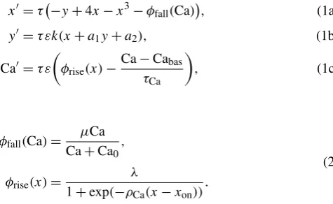
Figure2represents thex,y, and Ca patterns generated by system (1a)–(1c) with the set of parameter values given by Table1 except for μ set to 2, 2.4, and 3 in panel (a), (b), and (c), respectively. The generated Ca patterns reproduce different qualitative types of calcium patterns obtained experimentally in individual cells. In panels (a) and (b), the pattern is pulsatile but in panel (c), it is composed of a single isolated peak. In panel (a), there is no quiescent phase between successive peaks. In the case of panel (b), system (1a)–(1c) admits an attractive MMO limit cycle and the small oscillations reproduce the quiescent phase of the calcium pattern at the baseline level between two successive peaks.
Fig. 2 Patterns of variablesx,y, and Ca generated by system (1a)–(1c) with different values ofμ. The orbits correspond to types A, B and C described in the text and illustrated in Fig.1. The other parameter values were chosen according to Table1.a(μ=2): system (1a)–(1c) admits an attractive limit cycle of relaxation type. The increase in the calcium level is triggered by the activation ofx, the decrease by its deactivation. The Ca pattern is oscillatory and consists of successive peaks without any quiescent phase between two successive peaks.b(μ=2.4): system (1a)–(1c) admits an attractive MMO limit cycle. The quiescent phase after each Ca peak is due to small oscillations of the current point near the foldF−, which results in a slight and slow increase in Ca before the subsequent peak. The Ca pattern fulfills the average quantitative specifications provided by the experimental data.c(μ=3): starting from an initial condition just below the foldF−, the Ca pattern consists of a unique peak. Afterward, the current point(x, y,Ca)
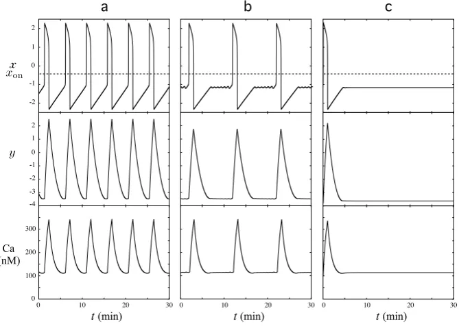
Fig. 3 Effects of changes in the value ofμandkon the IPI and peak heights of Ca patterns generated by system (1a)–(1c). The values ofμandkcorresponding to each colored pattern are given on the right of each panel. Ina, thered signalis obtained with parameter values given in Table1, the IPI equals 10 minutes and the height of the peaks is 342 nM (adashed red lineindicates this value inb,c, anddfor the sake of comparison).billustrates the effect of a change inμon the IPIs: theblue(resp.green)patternis obtained with a smaller (resp. larger) value ofμthan thered patternand has a smaller (resp. larger) IPI (7 minutes, resp. 14 minutes).cillustrates the effect of a change inkon the peak heights: an increase (resp. decrease) in the value ofk, as in theblue(resp.green)pattern, implies a decrease (resp. increase) in both the height of the peaks (320 nM, resp. 365 nM) and the IPI (around 4.5 minutes, resp. 17 minutes). Ind, we show how to hold the IPI constant (10 minutes) while obtaining a variability in the peak heights by changingkfirst (in the same way as inc) and then adjusting the value ofμ
3.2 Variability in Quantitative Properties of Calcium Patterns
In this section, we show how to mimic the variability of the quantitative features of calcium patterns between different cells by choosing different values for parameters of special importance:μandk. From the above explanation, one can already under-stand that the precise value ofμprescribes the number of small oscillations of the current point near the left foldF−and, consequently, the duration of the quiescent phase. Since variations inμdo not impact much the duration of the peaks, this pa-rameter can be considered to control the IPI. Panel (b) of Fig.3shows the results of a change inμ: an increase (resp. decrease) inμvalue implies an increase (resp. de-crease) in the IPI as shown by the green (resp. blue) pattern compared to the red one in panel (a). The range of variation inμis limited by the need to produce a quiescent phase between two successive peaks in the Ca pattern.
Parameterkessentially tunes the time scale separation betweenyand Ca (xbeing much faster). Hence, an increase ink implies a shorter time for subsystem (1a)– (1b) to complete a relaxation oscillation and, consequently, a shorter time for Ca to increase and decrease back to the baseline. One can thus increase or decrease the height of the Ca peak by tuning the value of parameterk. Of course, a change in
kalso implies a change in the duration of the quiescence phase and, consequently, the IPI. Panel (c) of Fig.3shows that an increase (resp. decrease) in the value ofk
implies a decrease (resp. increase) in the height of the peaks.
The peak height and the IPI can also be chosen independently by first tuning the value ofk and afterward the value ofμ. Panel (d) of Fig.3 shows the Ca patterns obtained with the same set ofk values as in panel (c) except that the values of μ
are chosen to balance the effect of the changes inkand maintain the 10 minutes IPI (μ=2.448 for the blue signal,μ=2.238 for the green one). Yet the variability in the peak heights persists.
The information on the dependence of the peak heights and the IPIs on the param-eters will be used to demonstrate the ability of our network model to reproduce the experimental results. Although we will not use this in the sequel, we would like to point out that other quantitative features could be controlled by tuning other parame-ters of system (1a)–(1c).
4 Network Model
In this section, we consider the following network model of a population of GnRH neurons:
xj =τ−yj+4xj−xj3−φfall(Caj)
, (6a)
yj =τ εkj
xj+a1yj+a2−ηjφsyn(σ )
, (6b)
Caj =τ ε
φrise(xj)−
Caj−Cabas
τCa
, (6c)
σ=τ
δεσ−γ (σ −σ0)φσ
1
N
N
i=1
Cai−Cadesyn
forj=1, . . . , N, withNthe number of neurons and
φsyn(σ )=
1
1+exp(−ρsyn(σ−σon))
,
φσ(u)=
1 1+exp(−ρσu)
.
(7)
In system (6a)–(6d), functionφσ is applied to
u= 1 N
N
i=1
Cai−Cadesyn,
which is the difference between the mean calcium level and the desynchronization threshold Cadesyn. For eachj=1, . . . , N, subsystem (6a)–(6c) (of the same type as
system (1a)–(1c)) represents the activity of thejth cell. The values of parameterskj are chosen randomly using a uniform distribution in the interval[0.8,1.2]to repro-duce, as explained in Sect.3, the variability in the IPI and height of the peaks from one cell to another. The values of the parameters that have been already introduced in Sect.3are given in Table1. Variableσ represents a global state of the network and acts on each cell through the termηjφsyn(σ ). Its dynamics consists of a very slow
linear part (εandδ are assumed to be small) and a term that depends on the level of synchronization of the network and acts as a reset mechanism when the network is sufficiently synchronized.
Note that the individual cells(xj, yj,Caj)are coupled only through variableσ which depends on the mean calcium concentration. This coupling is different from the one used in most synchronization studies and creates a link between calcium synchronization and higher calcium peaks. Similar global coupling arises in coupled arrays of Josephson junctions [14] as well as in a model of the Belusov–Zhabotinsky reaction with global feedback [15]. However, the specific feature of our coupling is that it is active only during very short periods when the mean calcium level is high.
Parameterσ0plays the role of a reset value and is chosen smaller thanσon.
Func-tions φsyn and φσ are increasing sigmoidal functions with inflection points at σon
and 0, respectively, and are both bounded above by 1. Since they play the role of activation functions, parametersρsynandφσ are assumed to be sufficiently large. In the limitρsyn→ +∞(resp.ρσ→ +∞),φsyn(resp.φσ) converges pointwise to the following Heaviside function with activation pointσon(resp. 0):
φsyn∞(σ )=H (σ−σon)= 0 if
σ < σon,
1 ifσ≥σon (8)
resp.φσ∞(u)=H (u)= 0 ifu <0,
1 ifu≥0
. (9)
4.1 Qualitative Study of the Network Model
Fig. 4 Transition of thejth cell of the network from independent to synchronized regime. In eachpanel, theblue partscorrespond to the unsynchronized regime,σ < σonandφsyn(σ )0, and thered partsto
the synchronized regime,σ > σonandφsyn(σ )1.aandbrepresent the projection of the orbit onto
the plane(xj, yj)forσ < σonandσ > σon, respectively, and the position of thexj andyj nullclines. Thexj nullcline depends on Caj: in eachpanel, the twocubic curvesrepresent thexj nullcline for the minimal (lower curve) and maximal (upper curve) value taken by Caj during the corresponding regime.
ctofrepresent the generatedxj, Caj, mean calcium (among all cells) andσpatterns. As long asσ < σon,
each cell generates a Caj pattern with it owns rhythm: the cells are asynchronous and the mean calcium level remains low (blue parts). Whenσexceedsσ0(red parts),φsyn(σ )is activated and the cells for which
ηiis large enough enter the steady regime (b). Hence, they produce, all almost at the same time, a higher calcium peak than in the asynchronous period of the oscillation. The mean calcium level exceeds Cadesyn,
which resetsσto a value close toσ0
driven transition of a particular cell of the network from the independent regime to the synchronized regime. Let us consider an initial value ofσ just aboveσ0. While
σ < σon,φsyn(σ )is almost zero and each cell (6a)–(6c) (forj=1, . . . , N) acts as
de-scribed in Sect.3. Since the values of parameterskjare different, each cell generates a Cajpattern with its own IPI. As a consequence, the calcium peaks are asynchronous and, as time evolves, the mean calcium level among cells, given by N1 Ni=1Cai, re-mains low. As long as the mean calcium level is smaller than Cadesyn, the second term
of theσ dynamics is negligible. Then, sinceδ is assumed to be small,σ increases very slowly. This regime corresponds to the orbit in blue shown in panel (a) of Fig.4
and the blue parts of the time series in panels (c) to (f).
Once the mean calcium level exceeds the threshold valueσon,φsyn(σ )activates.
Let us consider a particular cell, i.e., system (6a)–(6c) for a particular j. When
φsyn(σ )is activated, theyj nullcline quickly moves to the right and, provided that
ηj is large enough, ends up intersecting thexj nullcline on its right branch as shown on panel (b) of Fig.4. Hence, as long asφsyn(σ )is activated, the cell remains in a
higher than usual. Provided that sufficiently many cells are recruited in this process, the mean level quickly becomes higher than Cadesyn. This corresponds to the red parts
of the curves in Fig.4. Then the reset term of theσ dynamics activates,σ quickly decreases, crossing back the threshold valueσon, to a value nearσ0. Consequently,
φsyn(σ )is deactivated, and the whole process starts again.
It is worth noticing that all cells recruited in the event (i.e., those corresponding to a large enough value ofηj) were synchronized by the global variable to produce a higher calcium peak than usual. Moreover, they come back to their own pulsatile regime approximately at the same time, starting by a quiescence phase. Hence, all individual calcium levels are at the baseline for a while, before individual peaks rise again unsynchronized, which corresponds to a postexcitatory suppression.
4.2 Frequency of Synchronization Episodes
In Sect.3, we have shown how to specify the parameters of individual cells to obtain the required time traces. In this section, we show how to control the network level parametersσ0,σonandδto obtain global synchronization with a specified frequency.
In Proposition1, we prove that the evolution ofσ depends on the ratioσon/σ0rather
than on each of these parameters independently. Proposition2gives a formula for the dependence of the frequency of the synchronized peaks onδandσon/σ0.
Proposition 1 For any givenα >0,the outputsCajof system(6a)–(6d)are invariant under the change of parameter values from(σ0, σon, ρsyn)to(ασ0, ασon,
ρsyn
α ).
Proof Changing the parameters from(σ0, σon, ρsyn)to(ασ0, ασon,ρsynα )in system
(6a)–(6d) yields
xj =τ−yj+4xj−xj3−φfall(Caj)
, (10a)
yj =τ εkj
xj+a1yj+a2−ηjφsyn(σ )
, (10b)
Caj=τ ε
φrise(xj)−
Caj−Cabas
τCa
, (10c)
σ=τ
δεσ−γ (σ−ασ0)φσ
1
N
N
i=1
Cai−Cadesyn
, (10d)
where the new functionφsynis given by
φsyn(σ )=
1
1+exp(−(ρsyn/α)(σ−ασon))
. (11)
Changingσ toασ, and using the relation
φsyn(ασ )=φsyn(σ )=
1
1+exp(−ρsyn(σ−σon))
, (12)
Remark 1 As explained at the beginning of the section, the value ofρsyn is chosen
large enough so that the activation ofφsynis almost immediate. It is worth noticing
that a change in this value, provided that it remains large (typically greater than 10), does not affect the qualitative features of the model outputs (periodic episodes of syn-chronization) and has a limited impact on the period between two successive episodes of synchronization. Proposition1shows that, forρsynlarge enough and a fixed value
ofδ, the period of the synchronization episodes depends mainly on the ratioσon/σ0.
On the other hand, the value of these parameters can be chosen arbitrarily (provided thatσ0< σon) and the synchronization period can be adjusted by choosing the value
ofδas proved in Proposition2.
Proposition 2 In the caseρσ= ∞,forγ large enough relative toεandδ,the period
between two successive episodes of synchronization in system(6a)–(6d)is approxi-mated by
Tsyn=
1
τ εδln σon
σ0
. (13)
Remark 2 If the values of all the parameters of system (6a)–(6d), exceptδ, are fixed, we can adjust the synchronization period in the Caj pattern to any valueTsyn>0 by
choosing
δ= 1 τ εTsyn
lnσon
σ0
Proof of Proposition2 As explained above, each episode of synchronization results in a decrease ofσ, under the influence of the calcium dependent part of its dynamics. For a value ofγ large compared toεandδ, theσ dynamics, in the period whenφσ is active, is much faster than the Caj dynamics. Sinceρσ= ∞,σ decreases quickly down to a value very close to the singular pointσ of its dynamics defined by
δεσ−γ (σ−σ0)=0
i.e.,
σ= γ σ0
γ−δε=σ0+O
εδ γ
.
Hence, the timeTsyn between two successive synchronization episodes is
approxi-mately given by the time needed forσ to increase fromσ0up toσon. Let us recall
that the cells are asynchronous during this phase and
φ∞σ 1 N N
i=1
Cai−Cadesyn
=0.
It follows that, forσ < σon, theσ dynamics is given by its linear part:σ=δεσ. By
direct integration, one obtains
σ0exp(τ εδTsyn)=σon ⇔ Tsyn=
1
τ εδln σon
σ0
. (14)
Table 2 Parameter values of the network model (6a)–(6d) for generating full synchronization episodes
δ=0.05,
ρsyn=5,
γ=20,
ρσ=30,
ηj=3,
σon=60,
Cadesyn=350, σ0=0.1.
5 Three Types of Synchronization Episodes
In this section, we first show the ability of the model described by system (6a)–(6d) to reproduce sequences of synchronization events separated by asynchronous oscil-lations of the individual cells. We apply the results of Propositions1and2to control the periods and patterns of both the individual oscillations and the synchronized cal-cium peaks. Subsequently, we consider the question of introducing heterogeneity in the values of parametersηj, since they modulate the influence of the global variable
σ on thejth cell. This heterogeneity allows us to account for the additional feature of partial recruitment. We also show that parametersηj can be selected so that the desynchronization mechanism is weaker, which may lead to doublets of synchroniza-tion. In Sect.5.1, we discuss the case of full synchronization with no doublets, which corresponds to equal, sufficiently large values ofηj. In Sect.5.2, to obtain partial syn-chronization, we introduce unequal values ofηj including ones that are sufficiently small, so that the corresponding cells are not recruited by the synchronization mech-anism. In Sect.5.3, in order to obtain doublets of synchronization, we choose the values ofηj so that thexj andyj nullclines intersect near the upper fold of thexj nullcline. In this case, we choose in addition a relatively small value of parameterγ
to impose a slow decrease of the global variableσ.
5.1 Full Synchronization of Intracellular Calcium Peaks in a Network of GnRH Cells
In Table2, we introduce the values of the network level parameters for system (6a)– (6d). The valueδ=0.05 is obtained from equation (13) usingTsyn=60 min and
the parameter values of Table2. Moreover, for now, the same value is used for all parametersηj, so that the effect ofσ on each cell is the same. The value of Cadesyn
is chosen just above the mean calcium peak height of individual Caj pattern (i.e., the one generated by the three-dimensional system (1a)–(1c) with parameter values in Table1). This ensures that random synchronization between few cells will not interrupt the slow increase ofσ as the mean calcium level among all cells will not exceed Cadesyn. This happens only if a sufficient number of cells generate at the same
time a greater calcium peak than usual.
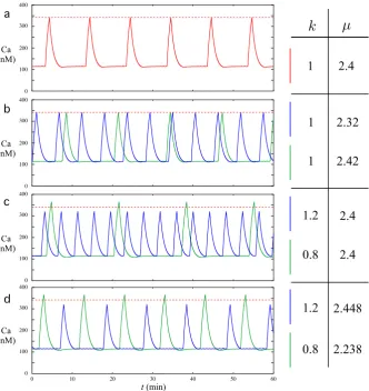
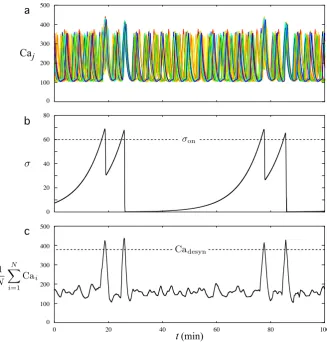
Fig. 5 Patterns of calcium oscillations in a network of 50 GnRH neurons.Ten different colorshave been used; eachcoloris used to represent the activity of 5 individual cells.arepresents the 50 individual Caj patterns along a 180 minute period. Note that synchronization occurred at minute 17, 78, and 139, which gives 61 minute intervals between synchronizations. The height of the synchronized peaks is larger than the height of normal peaks, and the postexcitatory suppressions are seen right after each synchronization episode.bdisplays a magnified view of the asynchronous phase occurring between successive episodes of synchronization. The Caj patterns display variability in IPI and height of the peaks between cells. Depending on the phases of each cell when the synchronization is triggered, the calcium peaks may be more or less tightly synchronized as emphasized incandd
Panels (c) and (d) show magnified views of two synchronization episodes. All cells are recruited in both episodes, resulting in higher calcium peaks than usual for all cells followed by complete postexcitatory suppression.
Note that the calcium peaks can be more or less tightly synchronized from one syn-chronization episode to another along the same trajectory of system (6a)–(6d). The extent of tightness can be assessed, following [4], as the length of the time interval with end points given by the time instances of the earliest and latest peak correspond-ing to a given synchronization event. In the synchronization episodes displayed in panels (c) and (d), this length equals 37 and 13 seconds, respectively. The variability in the tightness between different synchronization episodes is related to the maximum of the phase differences between each couple of oscillators (6a)–(6c) when the syn-chronization is triggered. Moreover, the time needed by each Caj to decrease back to the quiescent phase also depends on the relative positions of thexj andyj nullclines whenφsyn(σ )is activated. These positions are mainly characterized by the values of
differ-Fig. 6 Patterns of calcium oscillations in the 50 GnRH cells of a network with various sensitivity to the synchronization process.Ten different colorshave been used; eachcoloris used to represent the activity of 5 individual cells. Ina, the Caj patterns in all cells are shown for a period of 100 minutes. Only a part of the cells participates in the synchronization episodes att17 minutes andt76 minutes. The three other panelsdisplay magnified views of the second synchronization episodes by assembling the Caj patterns in cells, which are completely recruited in this event (b), recruited with no significant increase in the peak level (c) or not recruited at all (d)
ences between cells and the sensitivity to the synchronization mechanism interact in an intricate way, the precise study of the tightness of synchronization is a challenging problem.
5.2 Partial Recruitment
As mentioned in the preceding section, parameterηj tunes the impact of variable
σ upon the corresponding 3D system (6a)–(6c). Hence, it represents the sensitivity of the cell to the impact of the network state. One can mimic the variability in this sensitivity among cells by choosing different values ofηj.
Table 3 Parameter values of the network model (6a)–(6d) for generating synchronization as doublets
δ=0.05,
ρsyn=5,
γ=0.3,
ρσ=30,
ηj=1.12,
σon=60,
Cadesyn=380, σ0=0.1.
significantly higher than usual: their Caj patterns are assembled in panel (b). For 18 other cells (panel (c)), the Caj peaks are not significantly higher than usual, even if they are synchronized with those in panel (b). These cells corresponds to intermediate values ofηj. Moreover, in these Cajpatterns, the last IPI before the synchronization episode is much shorter than usual, which indicates that it does not result from a random coincidence but the cells actually undergo the effect of the synchronization process. Finally, the Caj patterns of the 12 remaining cells with low values ofηj (panel (d)) are not recruited by the synchronization mechanism: their peak heights are unchanged, their IPI remains constant during the synchronization episode and the calcium level can even be at the baseline.
5.3 Doublets
As explained in Sect.4, the reset mechanism ofσ is introduced through a fast part of the dynamics activated by the synchronization of the calcium peaks. The strength of this mechanism is controlled by the value of parameterγ and, in contrast with a classical reset, the decrease ofσ can be tuned by choosing the range ofγ values. In the preceding simulations, the values ofγ were chosen large enough (compared toε) so that, through the reset mechanism, σ can decrease down to a value very close toσ0before the mean calcium level decreases below the threshold Cadesyn. In
the following, we show how to reproduce doubled episodes of synchronization by slowing down theσ decrease induced by the synchronization of calcium peaks, i.e. by choosing a smaller value ofγ.
To ensure that, after the episode of synchronization, the mean calcium level de-creases as soon asσ starts to decrease, we select small enough values ofηj. For the sake of simplicity, we consider the same value for allηj,j =1, . . . , N, since the phenomenon of synchronization as doublet does not require variability in the cell sensitivity to synchronization. Hence, we consider the set of parameter values given in Table3.
Figure7 represents the outputs of system (6a)–(6d) using the parameter values given in Table3. The Caj patterns show synchronization episodes occurring as dou-blets. The first episode of synchronization occurs around minute 19 whenσ becomes greater thanσon. The tightness of this synchronization event is quite long, around 50
seconds. Consequently, the corresponding peak in the mean calcium level is not much higher than the asynchronous peaks. Whenσ decreases belowσon, the mean
cal-cium level decreases and quickly becomes smaller than Cadesyn. Parameterγis small
enough so that theσ reset mechanism is not entirely completed:σ starts increasing again from a value much greater thanσ0. Hence, a second episode of
Fig. 7 Synchronization as doublets in patterns of calcium oscillations in the 50 GnRH cells of a network. The parameter values of system (6a)–(6d) are given in Tables1and3. Ina,ten different colorshave been used to represent the Cajpatterns, hence each color is used to represent the activity of 5 individual cells.
brepresents the corresponding patterns ofσ as well as the synchronization thresholdσon(dotted line). crepresents the mean calcium level N1Ni=1Cai as well as the threshold Cadesyn(dotted line) which
triggers the decrease ofσ. Doublets of synchronization occur at minutes 19–26 and minutes 78–86: the two first episodes of synchronization are separated by a 60 minute period. The doublets occur because, after the first episode has been triggered, the mean calcium value stays above the threshold Cadesynonly
during a short time and, since theγ value is small,σ starts increasing again before reachingσ0vicinity.
Consequently, the subsequent synchronization episode occurs only 7 minutes afterward. It is worth notic-ing that the synchronization durnotic-ing the second episode of each doublet is tighter than durnotic-ing the first one. Hence, the subsequent decrease inσ is stronger than the preceding one, which results into a 56 minute period before the following doublet
higher than the first one. Subsequently, the time needed for the mean calcium level to decrease below Cadesyn is long enough for theσ reset mechanism to be completed.
Since variableσ slowly increases again from a value close toσ0, the subsequent
Note that the time separating two synchronization episodes of a doublet depends strongly on the value of parameterγ and the tightness of synchronization of the first episode. There is a strong variability in this duration from one doublet to another in a same set of Caj patterns. Hence, reproducing a given sequence of doublet is a chal-lenging problem. It is worth noticing that the variability in the doublets reproduced with the model is consistent with the variability observed in the experimental data [4].
6 Discussion
In this paper, we have presented a network model capable of reproducing the salient features of calcium oscillations that were observed by Terasawa and coworkers [3–
5] in their experiments on GnRH neurons in placode cultures. As observed in the experiments and recovered by our model, individual cells oscillate independently, with a significant variation in the oscillatory pattern. Superimposed on the individ-ual oscillations are synchronized events that can be described as almost simultaneous occurrences of calcium peaks, typically higher than in the absence of synchroniza-tion. Our model can reproduce these features in a very efficient way: By changing the parameters according to very simple rules, we can design the individual patterns of oscillation as well as control the frequency of the synchronization events. In addi-tion, we can reproduce the phenomena of partial recruitment and irregularities of the synchronization patterns, for example doubled episodes of synchronization.
To reproduce the irregularity of the individual oscillations a set of parameters con-trolling the individual patterns is drawn at random before each simulation. As the cells are coupled only during the synchronization episodes, the individual phases appear from the simulation to be completely ergodic. This may also be related to our choice of the parameters, corresponding to the sensitive dynamics of MMOs. Introducing even weak coupling between the cells might lead to some phase locking between the patterns, thus making the phases less irregular. This in turn could be destroyed by adding external noise. In this study, we have chosen not to include these effects.
effectively mobilized in embryonic neurons [25], we can only speculate on that issue. Following [26], we could conjecture that this effect is mediated through the nonneu-ronal cells that also exhibit calcium oscillations [5] and signal to GnRH neurons via ATP (Adenosine Triphosphate) through the ionotropic receptor P2X (a ligand-gated ion channel). The pharmacological control of ATP levels alters both synchronized calciums peaks and GnRH release. Hence, the synchronized peaks in GnRH neurons might be associated with a CICR mechanism induced by ATP inputs coming from the nonneuronal cells.
Other works have dealt with modeling the individual dynamics of GnRH neurons, representing the activity of the membrane potential and the ionic channels, in the style of the Hodgkin–Huxley system; see [27] for a study of GnRH neurons in brain slices from adult mice. A way to link our study to microscopic modeling of this kind could be by means of developing a firing rate model that would, in a similar way as our model, accurately reproduce the slow and super-slow timescales of individual and synchronized calcium oscillations as well as could be derived from a detailed microscopic model by means of averaging.
The main goal of this paper has been to design a model of coupled oscillators that could reproduce the experimental results of Terasawa [3] and in which we could iden-tify the parameters controlling the most relevant features of the experimental obser-vations, mainly the durations of the intervals separating the individual calcium peaks and synchronization events. Similar results may have been obtained by a different ap-proach, for example by adapting a model of population spikes [28], in which episodic synchronous spikes arise due to the presence of slowly varying parameters that make the system oscillate between the regions of synchronization and asynchronous behav-ior. A very useful feature of our model that may be difficult to obtain in such settings is the simple dependence of both the periods of the individual calcium peaks and synchronization events on the system parameters.
Finally, we would like to mention an aspect of the dynamics that our model was not designed to reproduce, namely a spatial structure in the patterns of spatial syn-chronization; see Fig. 4 in [4]. Spatial structures of calcium dynamics can be studied in continuous models; see, e.g., [29] for a study in the context of CICR. Spatial pat-terns registered by Terasawa and coworkers could possibly be understood in a mean field model derived from our network system.
Competing Interests
The authors declare that they have no competing interests.
Authors’ Contributions
FC identified the modeling issue and designed the biological specifications. MK conceived and built the model. AV improved and calibrated the model and performed the simulations. All authors participated in writing the manuscript. All authors read and approved the final manuscript.
References
1. Jasoni CL, Romanò N, Constantin S, Lee K, Herbison AE:Calcium dynamics in gonadotropin-releasing hormone neurons.Front Neuroendocrinol2010,31:259-269.
2. Moenter SM:Identified GnRH neuron electrophysiology: a decade of study.Brain Res2010,
1364:10-24.
3. Terasawa EI, Schanhofer WK, Keen KL, Luchansky L:Intracellular Ca2+oscillations in luteiniz-ing hormone-releasluteiniz-ing hormone neurons derived from the embryonic olfactory placode of the rhesus monkey.J Neurosci1999,19:5898-5909 [http://www.jneurosci.org/content/19/14/5898.full]. 4. Terasawa EI, Keen KL, Mogi K, Claude P:Pulsatile release of luteinizing hormone-releasing
hormone (LHRH) in cultured LHRH neurons derived from the embryonic olfactory placode of the rhesus monkey.Endocrinology1999,140:1432-1441 [http://endo.endojournals.org/content/ 140/3/1432.full].
5. Richter TA, Keen KL, Terasawa E: Synchronization of Ca2+ oscillations among primate LHRH neurons and nonneuronal cells in vitro. J Neurophysiol 2002, 88(3):1559-1567 [http://jn.physiology.org/content/88/3/1559.full].
6. Abe H, Terasawa E:Firing pattern and rapid modulation of activity by estrogen in primate luteinizing hormone releasing hormone-1 neurons.Endocrinology2005,146(10):4312-4320. 7. Nunemaker CS, Straume M, DeFazio RA, Moenter SM:Gonadotropin-releasing hormone neurons
generate interacting rhythms in multiple time domains.Endocrinology2003,144:823-831. 8. Pikovsky A, Rosenblum M, Kurths J:Synchronization: A Universal Concept in Nonlinear Sciences.
Volume 12. Cambridge: Cambridge University Press; 2003.
9. Malkin IG:Some Problems in Nonlinear Oscillation Theory. Moscow: Gostexizdat; 1956 (in Rus-sian).
10. Kopell N, Ermentrout GB:Symmetry and phaselocking in chains of weakly coupled oscillators. Commun Pure Appl Anal1986,39(5):623-660.
11. Hansel D, Mato G, Meunier C:Synchrony in excitatory neural networks.Neural Comput1995,
7(2):307-337.
12. Kuramoto Y:Chemical Oscillations, Waves, and Turbulence. Berlin: Springer; 1984.
13. Mirollo R, Strogatz S:Synchronization of pulse-coupled biological oscillators.SIAM J Appl Math 1990,50(6):1645-1662.
14. Hadley P, Beasley RM, Wiesenfeld K:Phase locking of Josephson-junction series arrays.Phys Rev B1988,38:8712-8719.
15. Rotstein HG, Kopell N, Zhabotinsky AM, Epstein IR:Canard phenomenon and localization of oscillations in the Belousov–Zhabotinsky reaction with global feedback.J Chem Phys2003,
119:8824-8832.
16. Börgers C, Kopell N:Synchronization in networks of excitatory and inhibitory neurons with sparse, random connectivity.Neural Comput2003,15(3):509-538.
17. Grynkiewicz G, Poenic M, Tsien GY:A new generation of Ca2+indicators with greatly improved fluorescence properties.J Biol Chem1985,26:3440-3450.
18. FitzHugh R:Impulses and physiological states in theoretical models of nerve membrane.Biophys J1961,1:445-466.
19. Ermentrout B, Pascal M, Gutkin B:The effects of spike frequency adaptation and negative feed-back on the synchronization of neural oscillators.Neural Comput2001,13(6):1285-1310. 20. Benoit E, Callot JL, Diener F, Diener M:Chasse au canard.Collect Math1981,31:37-119. 21. Desroches M, Guckenheimer J, Krauskopf B, Kuehn C, Osinga H, Wechselberger M:Mixed-mode
oscillations with multiple time scales.SIAM Rev2012,54:211-288.
22. Krupa M, Vidal A, Desroches M, Clément F:Multiscale analysis of mixed-mode oscillations in a slow–fast phantom bursting model.SIAM J Appl Dyn Syst2012,11:1458-1498.
23. Krupa M, Popovic N, Kopell N:Mixed-mode oscillations in three timescale systems—a prototyp-ical example.SIAM J Appl Dyn Syst2008,7:361-420.
24. Dupont G, Combettes L, Bird GS, Putney JW:Calcium oscillations.Cold Spring Harb Perspect Biol 2011,3:a004226.
25. Constantin S:Physiology of the gonadotrophin-releasing hormone (GnRH) neurone: studies from embryonic GnRH neurones.J Neuroendocrinol2011,23:542-553.
27. Lee K, Duan W, Sneyd J, Herbison AE:Two slow calcium-activated afterhyperpolarization cur-rents control burst firing dynamics in gonadotropin-releasing hormone neurons.J Neurosci 2010,30(18):6214-6224.
28. Mark S, Tsodyks M:Population spikes in cortical networks during different functional states. Front Comput Neurosci2012,6:43.