New inexact explicit thresholding/shrinkage formulas for inverse problems with overlapping group sparsity

R E S E A R C H

Open Access

New inexact explicit thresholding/

shrinkage formulas for inverse problems

with overlapping group sparsity

Gang Liu

, Ting-Zhu Huang

, Xiao-Guang Lv

and Jun Liu

Abstract

The least-square regression problems or inverse problems have been widely studied in many fields such as

compressive sensing, signal processing, and image processing. To solve this kind of ill-posed problems, a regularization term (i.e., regularizer) should be introduced, under the assumption that the solutions have some specific properties, such as sparsity and group sparsity. Widely used regularizers include the1norm, total variation (TV) semi-norm, and so on. Recently, a new regularization term with overlapping group sparsity has been considered. Majorization minimization iteration method or variable duplication methods are often applied to solve them. However, there have been no direct methods for solving the relevant problems due to the difficulty of overlapping. In this paper, we proposed new inexact explicit shrinkage formulas for one class of these relevant problems, whose regularization terms have translation invariant overlapping groups. Moreover, we apply our results to TV deblurring and denoising problems with overlapping group sparsity. We use alternating direction method of multipliers to iteratively solve them. Numerical results verify the validity and effectiveness of our new inexact explicit shrinkage formulas.

Keywords: Overlapping group sparsity, Total variation, ADMM, Image deblurring, Regularization, Explicit shrinkage formula

1 Introduction

The least-square regression problems or inverse prob-lems have been widely studied in many fields such as compressive sensing, signal processing, image process-ing, statistics, and machine learning. Regularization terms

with sparse representations (for instance, the1norm

reg-ularizer) have been developed into an important tool in these applications, and a list of methods have been pro-posed [1–4]. These methods are based on the assumption that signals or images have a sparse representation, that is, only containing a few nonzero entries. The corresponding task is to solve the following problem

min

z z1+

β

2z−x

2

2, (1)

*Correspondence: [email protected]

2Research Center for Image and Vision Computing/School of Mathematical Sciences, University of Electronic Science and Technology of China, Xiyuan Ave, 611731 Chengdu, China

Full list of author information is available at the end of the article

where x ∈ Rn is a given vector, z ∈ Rn, zp =

n

i=1|zi|p 1

p _with(_p = _{1, 2}) _{represents the}

p norm of

vectorz. The first term of (1) is called the regularization

term, the second term is called the fidelity term, andβ >0 is the regularization parameter.

To further improve the solutions, recent studies sug-gested to go beyond sparsity and took into account addi-tional information about the underlying structure of the solutions [1, 2, 5]. In particular, a wide class of solutions which have specific “group sparsity” structure are consid-ered. In this case, a group sparse vector can be divided into groups of components satisfying (a) only a few of groups contain nonzero values and (b) these groups are not needed to be sparse. If we insert such group vectors into a matrix as row vectors of the matrix, this matrix will only have few nonzero rows and these rows may be not sparse. This property is called “group sparsity” or “joint sparsity,” and many literature have considered these new sparse problems [1–6]. These problems can be for-mulated as the following expression.

min

z r

i=1

z[i]2+β

2z−x

2

2, (2)

where |zi| is the absolute value ofzi, andz[i] is theith

group ofzwithz[i]∩z[j]= ∅andr_i=1z[i]= z. “Group sparsity” solutions from (2) have better representation and have been widely studied both for convex and nonconvex cases [1, 3, 6–9].

More recently, overlapping group sparsity (OGS) have been considered [1, 3, 10–19]. These methods are based on the assumption that signals or images have a special sparse representation with OGS. The task is to solve the following problem

min

z z2,1+ β

2z−x

2

2, (3)

wherez2,1=n_i=1(zi)g2is the generalized2,1norm.

Here, each (zi)g is a group vector containing s (called

group size) elements that surrounding theith entry ofz.

For example,(zi)g=(zi−1,zi,zi+1)withs=3. In this case, (zi)g,(zi+1)g, and(zi+2)gcontain the(i+1)th entry ofz,

zi+1, which means “overlapping” different from the form

of group sparsity in (2). In particular, ifs = 1, the

gen-eralized2,1norm degenerates into the original1norm,

and the relevant regularization problem (3) degenerates to (1).

To be more general, researchers considered the

weighted generalized 2,1 normzw,2,1 = ni=1wg ◦

(zi)g2 (we only consider that each group has the same

weight, which means translation invariant) instead of

the former generalized 2,1 norm. The task can be

extended to

min

z zw,2,1+ β

2z−x

2

2, (4)

where wg is a nonnegative real vector with the same

size as (zi)g and “◦” is the point-wise product or

Hadamard product. For instance, wg◦(zi)g = ((wg)1zi, (wg)2zi+1,(wg)3zi+2) withs = 3 as the former example.

In particular, the weighted generalized2,1 norm

degen-erates into the generalized2,1 norm if each entry ofwg

equals to 1.

The problems (3) and (4) have been considered in [1, 14–19]. They solve the relevant problems by using variable duplication methods (variable splitting, latent/auxilliary variables, etc.). For example, Deng et al.

in [1] introduced a diagonal matrix Gin their method.

However, matrixGis not easy to find and would break the

structure of the coefficient matrix, which makes the diffi-culty of solving solutions under high-dimensional vector cases. Moreover, it is difficult to extend this method to the matrix case.

Considering the matrix case of the problem (4), we can get

min

A AW,2,1+ β

2A−X

2

F, (5)

where X,A ∈ Rm×n, AW,2,1 = mi=1

n

j=1Wg ◦ (Ai,j)gF. Here, each(Ai,j)g is a group matrix containing

K1×K2 (called group size) elements that surround the

(i,j)th entry ofA. It is defined by

Wg◦(Ai,j)g= ⎡

⎢ ⎢ ⎢ ⎢ ⎢ ⎣

(Wg)1,1Ai−l1,j−l2 (Wg)1,2Ai−l1,j−l2+1 · · · (Wg)1,K2Ai−l1,j+r2

(Wg)2,1Ai−l1+1,j−l2 (Wg)2,2Ai−l1+1,j−l2+1 · · · (Wg)2,K2Ai−l1+1,j+r2

. . .

. .

. . .. ...

(Wg)K1,1Ai+r1,j−l2 (Wg)K1,2Ai+r1,j−l1+1 · · · (Wg)K1,K2Ai+r1,j+r2

⎤ ⎥ ⎥ ⎥ ⎥ ⎥ ⎦

∈RK1×K2_,

wherel1 = K1₂−1,l2 = K2₂−1,r1 = K₂1,r2 = K₂2

(withl1+r1+1=K1andl2+r2+1=K2) andxdenotes

the largest integer less than or equal tox. In particular, if

K2 = 1, this problem degenerates to the former vector

case (4). IfK1 =K2=1, this problem degenerates to the

original1regularization problem (1) for the matrix case.

Much more recently, Chen et al. [10] considered the problem (5) when (Wg)i,j ≡ 1 for i = 1,· · ·,K1, j =

1,· · ·,K2. They used an iterative algorithm to solve this

problem based on the principle of majorization min-imization (MM). Their experiments showed that their method on solving the problem (3) is more efficient than other variable duplication methods (variable split-ting, latent/auxilliary variables, etc.) [1, 14–19]. Although their method is efficient for computing the solution, it may cost more time since the solution is obtained after many iterations rather than a direct step computation.

detail can be referred to Section 4). Numerical results will show that our method can save more time with getting very similar results.

The outline of the paper is as follows. In Section 2, we deduce our explicit shrinkage formulas in detail for the OGS problems (3), (4), and (5). In Section 3, we pro-pose some extensions for these shrinkage formulas. In Section 4, we apply our results to image deblurring and denoising problems with OGS TV. Numerical results are given in Section 5. Finally, we conclude this paper in Section 6.

2 OGS shrinkage

2.1 Classic shrinkage

In this subsection, we will review the original shrinkage formulas and their principles, since our new explicit OGS shrinkage formulas are based on them. Firstly, we give the following definition.

Definition 1.Define shrinkage mappings Sh1and Sh2

fromRN×R+toRNby

Sh1(x,β)i=sgn(xi)max

|xi| −

1

β, 0

, (6)

Sh2(x,β)=

x

x2max

x2− 1

β, 0

, (7)

where the expression is taken to be zero when the second factor is zero, and “sgn” represents the signum function

indicating the sign of a number. More precisely, sgn(x)=0

ifx=0, sgn(x)= −1 ifx<0, and sgn(x)=1 ifx>0.

The shrinkage (6) is known as soft thresholding and occurs in many algorithms related to sparsity since it is the

proximal mapping for the1norm. The shrinkage (7) is

known as high-dimensional shrinkage formula. Now, we consider solving the following problems

min

z zp+

β

2z−x

2

2, p=1, 2. (8)

The minimizer of (8) with p = 1 is the following

equation.

arg min

z z1+

β

2z−x

2

2=Sh1(x,β). (9)

Due to the additivity and separability of both the 1

norm and the square of the 2 norm, Eq. (9) can be

deduced easily by the following formula:

min

z z1+

β

2z−x

2 2=

n

i=1

min

zi |

zi| +β

2|zi−xi|

2_.

(10)

The minimizer of (8) with p = 2 is the following

equation.

arg min

z z2+

β

2z−x

2

2=Sh2(x,β). (11)

This formula is deduced by the Euler equation of (8)

withp = 2. In particular, without consideringx = 0or

z=0, we obtain the following Euler equation.

β (z−x)+ z

z2 0, (12)

1+ 1

β

1

z2

z−x0. (13)

We can easily get that the necessary condition is that the vectorzis parallel to the vectorx. That is, _zz

2 =

x x2.

Substituting into (13) and consideringx = 0or z = 0,

we obtain the formula (7). More details can be referred to [20, 21].

Our new explicit OGS shrinkage formulas are based on these observations, especially the properties of additivity, separability, and parallelity.

Remarks 1.The problem (2) is easy to be solved by a

simple shrinkage formula, which is not used in this work. More details can be referred to [1, 22, 23].

2.2 The OGS shrinkage formulas

Now, we focus on the problem (3) firstly. The difficulty of this problem is “overlapping.” Therefore, we must take some special techniques to avoid “overlapping.” That is the point of our new explicit OGS shrinkage formulas.

It is obvious that the first term of the problem (3) is additive and separable. So if we find some relative rules such that the second term of the problem (3) has the same properties with the same variable as the first term, one approximate solution of (3) can be easily found similar as classic shrinkage.

Assuming periodic boundary condition (PBC) (bound-ary condition (BC) is necess(bound-ary in OGS functionals) is

used here, we observe that each entry zi of the vector

zwould appear exactly stimes in the first term.

There-fore, to hold on the uniformity of vectors z and x, we

need to multiply the second term bys. To maintain the

invariability of the problem (3), after some manipulations, we have

fm(z)=min

z z2,1+ β

2z−x

2 2

=min

z

n

i=1(zi)g2+ β

2ssz−x 2 2

=min

z

n

i=1(zi)g2+ β

2s

n

i=1(zi)g−(xi)g 2 2

=min

z

n

i=1

(zi)g2+ β

2s(zi)g−(xi)g 2 2

,

(14)

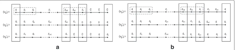
For example, we set s = 3 and define (zi)g = (zi,zi+1,zi+2). The generalized 2,1 norm z2,1 can be

treated as the generalized1norm of generalized points,

whose entry(zi)gis also a vector, and the absolute value

of each entry is treated as the2norm of(zi)g. See Fig. 1a

intuitively, where the top line is the vectorz, the

rectan-gles with dashed line are original(zi)g, and the rectangles

with solid line are the generalized points. In the case of PBC, we know that each line of Fig. 1a is translated equal.

We operate the vectorxsimilarly as the vectorz. Putting

these generalized points (rectangles with solid line in the figure) as the columns of a matrix, we can regardsz−x2₂ as the matrix Frobenius norm(zi)g

−(xi)g

2

F, where

(zi)g

is a matrix as in Fig. 1a with every line being its row ((xi)g

is similar). This is why the second equality in (14) holds.

Therefore, generally, for eachi of the last line of (14),

from the Eqs. (7) and (11), we can obtain

arg min

(zi)g(

zi)g2+ β

2s(zi)g−(xi)g 2 2=Sh2

(xi)g,β

s

,

(zi)g=max

(xi)g2− s

β, 0

₍

xi)g (xi)g2

,

(zi)g=

(zi)g

1,

(zi)g

2,. . .,

(zi)g

s

.

(15)

Similarly as Fig. 1a, for each i, the ith entry xi (or

zi) of the vector x (or z) may appear s times, so we

need to compute each zi for s times in s different

groups.

However, the results from (15) are not able to be

sat-isfied simultaneously, because the resultszi insdifferent

groups are different from (15). Moreover, for each i of

the last line in (14), the result (15) is given by that

the vector (zi)g is parallel to the vector (xi)g due to

Section 2.1.

Notice this point and ignore that(zi)g=0or(xi)g=0,

particularly fors= 4 and(zi)g = (zi−1,zi,zi+1,zi+2), the

vectorzcan be split as follows,

z= (z1, z2, z3, z4, z5, · · ·, zn−2, zn−1, zn ) = +1

4 (z1, z2, z3, 0, 0, · · ·, 0, 0,zn ) +1

4 (z1, z2, z3, z4, 0, · · ·, 0, 0, 0) +1

4 (0, z2, z3, z4, z5, · · ·, 0, 0, 0)

+ · · ·

+1

4 (z1, 0, 0, 0, 0, · · ·, zn−2, zn−1, zn ) +1

4 (z1, z2, 0, 0, 0, · · ·, 0, zn−1, zn ).

(16)

Let(zi)g = (0,· · ·, 0,zi−1,zi,zi+1,zi+2, 0,· · ·, 0)be the

expansion of (zi)g, with (z1)g = (z1,z2,z3, 0,· · ·, 0,zn), (zn−1)g = (z1, 0, 0,· · ·, 0,zn−2,zn−1,zn),(zn)g = (z1, z2, 0,· · ·, 0,zn−1,zn). Let (xi)g = (0,· · ·, 0,xi−1,xi,xi+1, xi+2, 0,· · ·, 0)be the expansion of(xi)gsimilarly as(zi)g.

Then, we have z = 1₄n_i=1(zi)g, and x = 14

n

i=1(xi)g.

Moreover, we can easily obtain that(zi)g2 = (zi)g2

and(xi)g2= (xi)g2for everyi.

On one hand, the Euler equation offm(z)(withs=4) is

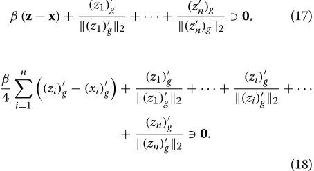
given by

β (z−x)+ (z1)

g (z1)g2

+ · · · + (zn)g (z_n)g2

0, (17)

β

4

n

i=1

(zi)g−(xi)g

+ (z1)g (z1)g2

+ · · · + (zi)g (zi)g2

+ · · ·

+ (zn) g (zn)g2

0.

(18)

From the deduction of the two-dimensional shrinkage formula (7) in Section 2.1, we know that the necessary condition of minimizing theith term of the last line in (14)

a

b

Fig. 1Vector case. Thetop lineis the vectorz, therectangles with dashed lineare original group vector(zi)g, and therectangles with solid lineare the

is that(zi)g is parallel to(xi)g. That is,(zi)g is parallel to (xi)gfor everyi. For example,

(z2)g=(z1,z2,z3,z4, 0,· · ·, 0, 0)//(x2)g=(x1,x2,x3,x4, 0,· · ·, 0, 0).

(19)

Then, we obtain (zi)g (zi)g2 =

(xi)g

(xi)g2. Therefore, (18) can

be changed to

β

4 n

i=1

(zi)g−(xi)g

+ (x1)g (x1)g2+ · · · +

(xi)g (xi)g2+ · · · +

(xn)g (xn)g2 0,

(20)

β (z−x)+ (x1)

g (x1)g2+ · · · +

(xi)g (xi)g2+ · · · +

(xn)g (xn)g2

0, (21)

zx−1_β

(x1)g (x1)g2 + · · · +

(xi)g (xi)g2+ · · · +

(xn)g (xn)g2

, (22)

for each component, we obtain

zixi−

1

β

xi (xi−2)g2

+ xi

(xi−1)g2

+ xi

(xi)g2

+ xi

(xi+1)g2

.

(23)

Therefore, when (zi)g = 0 and (xi)g = 0, we find

a minimizer of (3) on the direction that all the vec-tors (zi)g are parallel to the vectors (xi)g. In addition,

when β₄

(zi)g−(xi)g

+ (zi)g

(zi)g2 = 0, (18) holds, then

β

4 +(zi1)g2

(zi)g = (xi)g; therefore,

(zi)g (zi)g2 =

(xi)g (xi)g2

holds. Moreover, because of the strict convexity offm(z),

we know that the minimizer is unique.

On the other hand, when(zi)g = 0or (xi)g = 0, our

method may not obtain good results. When(xi)g=0, we

know that the minimizer of the subproblem min

(zi)g(

zi)g2+

β

2s(zi)g−(xi)g22is exactly that(zi)g = 0. When(xi)g =

0 and the minimizer of the subproblem min

(zi)g

(zi)g2+

β

2s(zi)g−(xi)g22is that(zi)g = 0(since the parameter

β/sis two small), our method is not able to obtain good

results. For example, that (zi)g = 0while (zi+1)g = 0

makes the element zi in z take different values in

dif-ferent subproblems. However, we can obtain an approx-imate minimizer in this case, which is that the element

zi is a simple summation of corresponding subproblems

containing zi. We will show that in the experiments of

Section 5, the approximate minimizer is also good. More-over, when we take this problem as a subproblem of the

image processing problem, we can set the parameterβto

be large enough to avoid this drawback.

In addition, from (23), we can know that the elementzi

of the minimizer can be treated as inssubproblems

inde-pendently and then we combine them. In conclusion, after some manipulations, we can get the following two general formulas.

(I)

arg min

z z2,1+ β

2z−x

2

2=ShOGS(x,β), (24)

with

ShOGS(x,β)i=zi=max

1− 1

βF(xi), 0

xi. (25)

Here, for instance, when group size s = 4, (zi)g =

(zi−1,zi,zi+1,zi+2) in z2,1 and (xi)g is defined

simi-larly as (zi)g, we have F(xi) =

1 (xi−2)g2 +

1 (xi−1)g2

+ 1

(xi)g2 +

1 (xi+1)g2

. The(xj)g2is contained inF(xi)

if and only if(xj)g2has the componentxi, and we follow

the convention(1/0) = 1 inF(xi)because(xi)g2 = 0

implies xi = 0 and the value of F(xi) is insignificant

in (25).

(II)

arg min

z z2,1+ β

2z−x

2

2=ShOGS(x,β), (26)

with

ShOGS(x,β)i=zi=G(xi)·xi. (27)

Here, symbols are the same as (I), and G(xi) =

max1_s − _β(x1

i−2)g2, 0

+ max1_s −_β(x1

i−1)g2, 0

+ max 1 s − 1

β(xi)g2, 0

+max 1 s − 1

β(xi+1)g2, 0

.

We call them Formula (I) and Formula (II) respectively

throughout this paper. Whenβis sufficiently large or

suf-ficiently small, the former two formulas are the same. For

the other values ofβ, from the experiments, we find that

Formula (II) is better approximate to the MM iteration method than Formula (I), so we list the algorithm for For-mula (II) as follows for finding the minimizer of (3). If we would use Formula (I), we can only change the final three steps, which does not change the computation cost.

We can see that Algorithm 1 only needs 2 times of

con-volution computations with time complexityn∗s, which is

just the same time complexity as one-step iteration in the MM method of [10]. Therefore, our method is much more efficient than the MM method or other variable dupli-cation methods. In Section 5, we will give the numerical experiments for comparison between our method and the

MM method. Moreover, ifs= 1, our Algorithm 1

degen-erates to the classic soft thresholding as our formula (27)

or sufficiently small, the results of our new explicit algo-rithm are almost the same as the MM method (after 20 or more iteration steps) in [10].

Algorithm 1 Direct shrinkage algorithm for the

mini-mization problem (3) Input:

Given vectorx=(x1,x2,· · ·,xn), group sizes,

parameterβ.

Compute:

1. Definition of(xi)g, for example(xi)g=xi−sl,· · ·,

xi,· · ·,xi+sr

, withsl=[s−₂1] andsr=[s₂] (sl+sr +1=s).

w= ones(1,s) = [1,1,· · ·,1].

Ifsis even, thenw=[w, 0] ands=s+1.

Letwr= fliplr(w) be flipingwover 180 degrees.

2. ComputeXn=

(x1)g2,· · ·,(xi)g2,· · ·,(xn)g2

,

by convolution ofwandx.

3. ComputeX_n =max1_s −1./(Xn·β), 0

point-wise. 4. ComputeG(xi)by correlation ofwandXn,

or by convolution ofwrandXn.

5. Computezby multiplyingxwithG(xi)point-wise.

Remarks 2.Our new explicit algorithm can be treated

as an average estimation algorithm for solving all the over-lapping group subproblem independently. In Section 5, our numerical experiments show that the results of our two formulas are almost the same as the MM method in

[10] whenβ is sufficiently large or sufficiently small and

is approximate to the MM method for otherβ. Moreover,

this point illuminates that the OGS regularizers coincide to maintain the property of the classical sparse regulariz-ers and smoothen the local regions. For instance, TV with OGS can preserve edges and simultaneously overcome staircases in our experiments and [11, 12].

For the problems (4) (See Fig. 1b intuitively) and (5), we can get similar algorithms. We omit the evolution details here and give them as in Appendix. Here, we directly give the algorithm for solving the problem (5) as follows under Formula (II).

We can also see that Algorithm 2 only needs 2 times

of convolution computations with time complexityn∗s,

which is just the same time complexity as one-step itera-tion in the MM method of [10]. Therefore, our method is much more efficient than the MM method.

3 Several extensions

3.1 Other boundary conditions

In Section 2, we gave the explicit shrinkage formulas for one class of OGS problems (3), (4), and (5). In order to

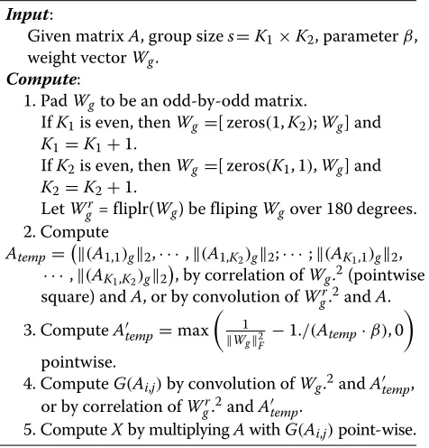
Algorithm 2 Direct shrinkage algorithm for the

mini-mization problem (4) Input:

Given matrixA, group sizes=K1×K2, parameterβ,

weight vectorWg.

Compute:

1. PadWgto be an odd-by-odd matrix.

IfK1is even, thenWg=[ zeros(1,K2);Wg] and K1=K1+1.

IfK2is even, thenWg=[ zeros(K1, 1),Wg] and K2=K2+1.

LetW_gr= fliplr(Wg) be flipingWgover 180 degrees.

2. Compute

Atemp=

(A1,1)g2,· · ·,(A1,K2)g2;· · ·;(AK1,1)g2,

· · ·,(AK1,K2)g2

, by correlation ofWg.2(pointwise

square) andA, or by convolution ofW_gr.2andA.

3. ComputeA_temp=max

1 Wg2

F −

1./(Atemp·β), 0

pointwise.

4. ComputeG(Ai,j)by convolution ofWg.2andAtemp,

or by correlation ofW_gr.2andA_temp.

5. ComputeXby multiplyingAwithG(Ai,j)point-wise.

achieve a simply deduction, we assume that PBC is used. One may confuse that whether PBC is always good for reg-ularization problems such as signal processing or image processing, since natural signals or images are often asym-metric. However, in these problems, assuming a kind of boundary condition is necessary for simplifying the prob-lem and making the computation possible [24]. There are kinds of BCs, such as zero BC (ZBC) and reflective BC. PBC is often used in optimization because it can be computed fast as above or other methods, for example, computation of matrix of block circulant with circulant blocks (BCCB) by fast Fourier transforms [20, 21, 24].

In this section, we consider other BC such as ZBC and reflective BC. For simplification, we only consider the vector case, while the results can be easily expanded to the matrix case as that in Section 2. When ZBC is used, we can expand the original vectors (or signal)

z (= (zi)ni=1) and x by two s-length vectors on the

both hands of the original vectors, which are z˜ (=

˜

z−s,· · ·,z˜−1,(˜zi)in=1,z˜n+1,· · ·,z˜n+s

= 0s,(zi)ni=1,0s

)

and x, respectively. Then, the results and algorithms in˜

Section 2 are similar as the case of PBC onz˜ andx. See˜

Fig. 2a intuitively.

Moreover, our numerical results will show that the results from a different BC are almost the same in prac-tice (see Section 5.1); and according to the definition of

weighted generalized2,1 norm, ZBC seems better than

a

b

Fig. 2The case of expanding vectors with other BCs to use the formulas under PBC.aZBC.bReflective BC

When reflective BC is assumed, the results are also the

same. We only need to extend the original vectorxtoxˆ

with reflective BC. See Fig. 2b intuitively.

3.2 Nonpositive weights and different weights in groups

In this section, we show that the weight vectorwg and

matrixWg in the former sections can contain arbitrary

sentries with arbitrary real numbers. On one hand, the

zero value can be the arbitrary entries of the weight

vec-tor or matrix. For example, the original1regularization

problem (1) can be seen as a special form of weighted

gen-eralized2,1norm regularization problems (4) withs=1

ors=3 andwg=(1, 0, 0)for the example of Fig. 1b.

On the other hand, the norm is with the property of

positive homogeneity,(−1)·wgany = wgany, where

“ · any” can be arbitrary norm such as · 1and · 2.

Therefore, for the regularization problems (4) (or (5)), the

weight vector wg (or matrixWg) is the same as|wg|(or

|Wg|), where| · |the point-wise absolute value. Therefore,

in general, our results are true, whatever the number of

entries included in the weight vectorwg and matrixWg

and whatever the real number value of these entries.

However, if the weightwg is dependent on the group

indexi, for example,wi,g ◦(zi)g =

(wi,g)1zi,(wi,g)2zi+1, (wi,g)3zi+2

, we cannot solve the relevant problems easily since our method fails. As we mentioned above, we only

focus on that the weightwgis independent on the group

indexi, that is,wi,g = wgfor alli, which means that it is

with translation invariant overlapping groups.

4 Applications in TV regularization problems with OGS

The TV regularizer was firstly introduced by Rudin et al. [25] (ROF), which is widely used in many fields, i.e., denoising and deblurring problems [20, 21, 26–31]. Sev-eral fast algorithms such as Chambelle [26] and fast TV deconvolution (FTVd) [20, 21] have been proposed. Its corresponding minimization task is

min

f fTV+ μ

2Hf−g

2

2, (28)

wherefTV:=

1≤i,j≤n

(∇f)i,j2= 1≤i,j≤n

|(∇xf)i,j|2+|(∇yf)i,j|2

(called isotropic TV, ITV), orfTV :=

1≤i,j≤n(∇

f)i,j1=

1≤i,j≤n|(∇x

f)i,j| + |(∇yf)i,j|(called anisotropic TV, ATV),

H denotes the blur matrix, and g denotes the given

observed image with blur and noise. Operator∇ :Rn2 →

R2×n2

denotes the discrete gradient operator (under PBC) which is defined by (∇f)i,j = ((∇xf)i,j,(∇yf)i,j),

with

(∇xf)i,j=

fi+1,j−fi,jif i<n,

f1,j−fn,j if i=n, (∇yf)i,j=

fi,j+1−fi,jif j<n, fi,1−fi,n if j=n,

fori,j = 1, 2,· · ·,n, wherefi,j refers to the((j−1)n+ i)th entry of the vector f (it is the (i,j)th pixel

loca-tion of then×nimage, and this notation remains valid

throughout the paper unless otherwise specified). Notice

that H is a matrix of BCCB structure when PBC are

applied [24].

Firstly, we define the ATV case with OGS under Gaus-sian noise and impulse noise respectively which is similar as [11, 12]. For the Gaussian noise case,

min

f (∇xf)W,2,1+ (∇yf)W,2,1+ μ

2Hf −g

2 2. (29)

For the impulse case,

min

f (∇xf)W,2,1+ (∇yf)W,2,1+μHf −g1. (30)

We call the former model as TV OGSL2model and the

latter model as TV OGSL1model, respectively.

Then, we defined the ITV case with OGS. For Gaussian noise and impulse noise, we only change the former two

terms of (29) and (30) respectively byAW,2,1. Here,A

is a high-dimensional matrix (or tensor) with each entry

Ai,j=((∇xf)i,j;(∇yf)i,j).

Remarks 3. In particular in this work,Acan be treated

as((∇xf);(∇yf))for simplicity in vector and matrix

com-putation, although the computation ofAW,2,1is should

be treated as pointwise withAi,j=((∇xf)i,j;(∇yf)i,j)since

the computation onAis almost all pointwise.

Moreover, we consider constrained model as listing in [11, 12, 32]. For any true digital image, its pixel value can attain only a finite number of values. Hence, it is natural to require all pixel values of the restored image to lie in a certain interval [a,b], see [32] for more details. In general, with the easy computation and the certified results in [32], we only consider all the images located on the standard

range [ 0, 1]. Therefore,we define a projection operatorP

on the set=f ∈Rn×n|0≤f ≤1,

P(f)i,j= ⎧ ⎨ ⎩

0, fi,j<0, fi,j, fi,j∈[ 0, 1] ,

1, fi,j>1.

(31)

4.1 Constrained TV OGSL2model

For the constrained model (the ATV case) (called CATVOGSL2), we have

min

u∈,vx,vy,f

(vx)W,2,1+ (vy)W,2,1+ μ

2Hf −g

2 2:

vx = ∇xf,vy= ∇yf,u=f

.

(32)

The augmented Lagrangian function [33] of (32) is

Lvx,vy,u,f;λ1,λ2,λ3= vxW,2,1−λT1(vx− ∇xf)+β1

2vx− ∇xf

2 2

+ vyW,2,1−λT2(vy− ∇yf)+β1

2vy− ∇yf

2 2

−λT

3(u−f)+

β2

2u−f

2 2+

μ

2Hf−g

2 2,

(33)

whereβ1,β2 > 0 are penalty parameters andλ1,λ2,λ3 ∈

Rn2_{are the Lagrange multipliers.}

The solving algorithm is according to the scheme of ADMM in Gabay [34], and we refer to some applica-tions in image processing which can be solved by ADMM, e.g., [35–43]. For a given vk_x,vk_y,uk,fk;λk₁,λk₂,λk₃, the

next iteration (vk+1

x ,vky+1,uk+1,fk+1;λk1+1,λ2k+1,λk3+1) is

generated as follows:

1. Fixf = fk,λ1 = λk1,λ2 = λk2,λ3 = λk3and minimize

(33) with respect tovx,vy, andu. With respect tovxandvy,

v_xk+1=arg minvxW,2,1−λk1 T

(vx−∇xfk)+β₂1vx−∇xfk22 =arg minvxW,2,1+β₂1vx− ∇xfk−λ

k

1

β1

2 2,

(34)

vk+1

y =arg minvyW,2,1−λk2 T

(vy−∇yfk)+β₂1vy−∇yfk22 =arg minvyW,2,1+ β₂1vy− ∇yfk−λ

k

2

β1

2 2.

(35)

It is obvious that problems (34) and (35) match the framework of the problem (5); thus, the minimizers of (34) and (35) can be obtained by using the formulas in Section 2.2.

With respect tou,

uk+1=arg min−λk₃T(u−fk)+ β2

2u−fk22 =arg minβ2

2u−fk−

λk

3

β2

2 2.

The minimizer is given explicitly by

uk+1=P

fk+λ k 3 β2

. (36)

2. Computefk+1_{by solving the normal equation}

(β1(∇x∗∇x+ ∇y∗∇y)+μH∗H+β2I)fk+1 = ∇∗

x(β1vkx+1−λk1)+ ∇y∗(β1vky+1−λk2)+μH∗g +β2(uk+1−λ

k

3

β2),

(37)

where “∗” denotes the conjugate transpose, see [44] for

more details. Since all the parameters are positive, the coefficient matrix in (37) are always invertible and sym-metric positive-definite. In addition,H,∇x,∇yand their

conjugate transpose have BCCB structure under PBC. We know that the computations with BCCB matrix can be very efficient by using fast Fourier transforms.

3. Update the multipliers via

⎧ ⎪ ⎨ ⎪ ⎩

λk+1

1 =λk1−γβ1(vxk+1− ∇xfk+1), λk+1

2 =λk2−γβ1(vxk+1− ∇xfk+1), λk+1

3 =λk3−γβ2(uk+1−fk+1).

Based on the discussions above, we present the ADMM algorithm for solving the convex CATVOGSL2 model (32), which is shown as Algorithm 3.

Algorithm 3CATVOGSL2 for the minimization problem

(32)

initialization:

Starting pointf0_=g,k=0,β

1,β2,γ,μ, group size K1×K2, weighted matrixWg,λ0_i =0,i=1, 2, 3.

iteration:

1. Computevk_x+1andv_yk+1according to(34)and(35). 2. Computeuk+1according to(36).

3. Computefk+1by solving(37).

4. updateλ0_i =0,i=1, 2, 3 according to(38).

5.k=k+1.

until a stopping criterion is satisfied.

Algorithm 3 is an application of ADMM for the case with two blocks of variables (vx,vy,u) and f. Thus, if

the step (1) of Algorithm 3 can be solved exactly, its convergence is guaranteed by the theory of ADMM [34, 35, 37, 43]. Although step (1) of Algorithm 3 can-not be solved exactly, we can find a convergent series to ensure the convergence as [35]. Besides, our numerical experiments verify the convergence of Algorithm 3.

Remarks 4.For the image f, we use PBC for the fast

computation. However, forvx,vy, we use ZBC. Becausevx

andvydenote the gradient of the image, ZBC seems better

for the definition of the generalized norm2,1onvxandvy

as mentioned in Section 3.1. Therefore, the two kinds of BCs for the image and its gradient are different and inde-pendent. These remain valid throughout the paper unless otherwise specified.

For the ITV case, the constrained model (CITVOGSL2) is

min

u∈,A,f

AW,2,1+μ

2Hf−g

2

2: A=(∇xf;∇yf),u=f

.

(39)

The detail will be presented in the next section for

the constrained TV OGSL1model. We call this relevant

algorithm CITVOGSL2.

4.2 Constrained TV OGSL1model

For the constrained model (the ITV case) (called CITVOGSL1), we have

min

u∈,A,f

AW,2,1+μz1:z=Hf−g,A=(∇xf;∇yf),u=f

.

(40)

The augmented Lagrangian function of (40) is

Lvx,vy,z,w,f;λ1,λ2,λ3,λ4= AW,2,1−

λT

1,λT2

A−

∇xf ∇yf

+β1 2

"" "" "A−

∇xf ∇yf

"" "" " 2

2 +μz1−λT3

z−(Hf−g) +β2

2z−(Hf−g) 2 2

−λT

4(w−f)+

β3 2w−f

2 2,

(41)

where β1,β2,β3 > 0 are penalty parameters and

λ1,λ2,λ3,λ4∈Rn

2

are the Lagrange multipliers. For a given (Ak,zk,uk,fk; λk

1,λk2,λk3,λk4), the next

iter-ation (Ak+1,zk+1,uk+1, fk+1; λ₁k+1,λk₂+1,λ₃k+1, λk₄+1) is generated as follows:

1. Fixf = fk,λ1 = λk1,λ2 = λk2,λ3 = λk3,λ4 = λk4and

minimize (41) with respect toA,z, andu. With respect to

A,

Ak+1_{=arg minA}

W,2,1−(λT1,λT2)(A−

∇xfk ∇yfk

)+β1

2

"" "" "A−

∇xfk ∇yfk

"" "" " 2 2 , Ak1+1

Ak2+1

=arg minAW,2,1+β21

"" "" " A1 A2 −

∇xfk ∇yfk

−

λk

1/β1

λk

2/β1

"" "" " 2 2 . (42)

It is obvious that problem (42) match the framework of the problem (5), thus the solution of (42) can be obtained by using the formulas in Section 2.2.

With respect toz,

zk+1=arg minμz1−λk3

T

z−(Hfk−g)+β2

2z−(Hfk−g)22 =arg minμz1+β22z−(Hfk−g)−

λk

3 β2

2 2.

The minimization with respect tozcan be given by (6)

and (9) explicitly, that is,

zk+1=sgn

#

Hfk−g+λ k 3 β2 $ ◦max #

|Hfk−g+λ k 3 β2| −

μ β2 , 0 $ . (43)

With respect tou,

uk+1=arg min−λk₄Tu−fk+ β3

2u−fk22 =arg minβ3

2u−fk−

λk

4

β3

2 2.

The minimizer is given explicitly by

uk+1=P

fk+λ k 4 β3

2. Compute fk+1 _{by solving the following normal}

equation similarly as the last section.

(β1(∇x∗∇x+ ∇y∗∇y)+β2H∗H+β3I)fk+1 = ∇∗

x(β1Ak₁+1−λk₁)+ ∇y∗(β1Ak₂+1−λk₂)+ H∗(β2zk+1−λk3)+β2H∗g+β3(uk+1− λ

k

4

β3).

(45)

3. Update the multipliers via

⎧ ⎪ ⎪ ⎪ ⎨ ⎪ ⎪ ⎪ ⎩

λk+1 1 λk+1

2 =

% λk

1 λk 2 &

−γβ1

Ak₁+1 Ak₂+1 −

% ∇xfk+1 ∇yfk+1

&

,

λk+1

3 =λk3−γβ2(zk+1−(Hfk+1−g)), λk+1

4 =λk4−γβ3(uk+1−fk+1).

(46)

Based on the discussions above, we present the ADMM algorithm for solving the convex CITVOGSL1 model (40), which is shown as Algorithm 4.

Algorithm 4CITVOGSL1 for the minimization problem

(40)

initialization:

Starting pointf0=g,k=0,β1,β2,β3,γ,μ, group size K1×K2, weighted matrixWg,λ0_i =0,i=1, 2, 3, 4.

iteration:

1. ComputeAk+1_{according to(42),}

and computezk+1according to(43). 2. Computeuk+1according to(44). 3. Computefk+1_{by solving(45).}

4. updateλ0_i =0,i=1, 2, 3, 4 according to(46).

5.k=k+1.

until a stopping criterion is satisfied.

Algorithm 4 is an application of ADMM for the case with two blocks of variables (A,z,u) andf. Thus, if step (1) of Algorithm 4 can be solved exactly, its convergence is guaranteed by the theory of ADMM [34, 35, 37, 43]. Although step (1) of Algorithm 4 cannot be solved exactly, we can find a convergent series to ensure the conver-gence as [35]. Besides, our numerical experiments verify the convergence of Algorithm 4.

For the ATV case, the constrained model

(CATVOGSL1) is

min

u∈,vx,vy,f

(vx)W,2,1+ (vy)W,2,1+μz1: z=Hf −g,vx= ∇xf,vy= ∇yf,u=f

.

(47)

The detail has been presented in the last section for

the constrained TV OGSL2model. We call this relevant

algorithm CATVOGSL1.

5 Numerical results

In this section, we present several numerical results to illustrate the performance of the proposed method. All experiments are carried out on a desktop computer using MATLAB 2010a. Our computer is equipped with an Intel Core i3-2130 CPU (3.4 GHz), 3.4 GB of RAM, and a 32-bit Windows 7 operation system.

5.1 Comparison with the MM method for one-dimensional signal denoising

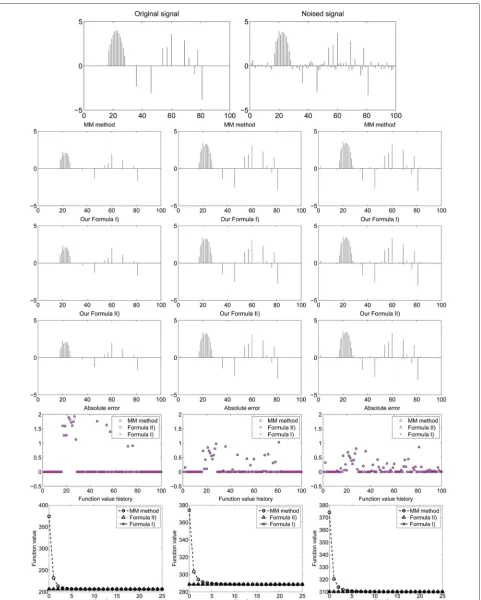
As an illustrative example, we apply our direct formulas in one-dimensional signal denoising. We only compare the results of our explicit shrinkage formulas with the most recent MM iteration method proposed in [10] as a

sim-ple examsim-ple. The one-dimensional group sparse signalz

is shown in the top left of Fig. 3. The noisy signalxin the

top right of Fig. 3 is obtained by adding independent white

Gaussian noise with standard deviationσ = 0.5 same as

[10]. The denoising model is as follows

arg min

z Fun(z)= z2,1+ β

2z−x

2

2. (48)

We test several different parametersβ(any integer from

1 to 50) for the comparison. The results of our formu-las are almost the same as the MM method for almost

theseβs. Due to the limit space, we only illustrate parts

of the results (β = 3, 10, 15) in Fig. 3. We take both our

Formulas (I) and (II) for the comparison with the MM method. From the figure, we can visually see that our results by our two kinds of formulas are almost the same

as the MM method for differentβ. Moreover, for the

prac-tical problems,β = 10, can be better than others from

the figure. This shows that our formulas are feasible, use-ful, and effective, because our method can only need the same computation cost as one-step iteration in the MM method while the MM method needs 25 iterations as [10]. That means our method is 25 times faster than the MM method. From the bottom line of Fig. 3, we can see that the MM method may take 5 iterations to be convergent, which is the reason why Liu et al. in [11] and Liu et al. in [12] only choose 5 inner iterations. However, in this case, our method is still 5 times faster than the MM method.

Remarks 5.Although this model is not the best model

for signal denoising, it shows the superiority of our method. Moreover, the authors in [10] also take similar experiments.

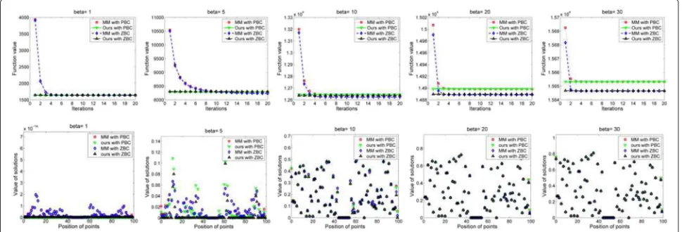
5.2 Comparison with the MM method on problem (5) In this section, we give another example by solving the matrix case problem (5) for comparison with the

MM method. Without loss of generality, we let A =

example. In particular, we set weighted matrix Wg ∈ R3×3_((W

g)i,j≡1) and list (5) again

fA(X)=min

X Fun(X)= X2,1+ β

2X−A

2 F. (49)

We use different parametersβ and use the number of

MM iteration by 20 steps. For comparison, we expand our result by explicit shrinkage formulas to length 20 (the same as the MM iteration steps). The values of the object function Fun(X) against iterations are illustrated in the top line in Fig. 4. The cross-sectional elements of the

mini-mizerAare shown in the bottom line in Fig. 4. We choose

both ZBC and PBC for our method and the MM method. It can be seen that there is only a little difference between the two kinds of BCs.

It is obvious that our method is much more efficient than the MM method since our time complexity is just the same as one-step iteration in the MM method due to the explicit shrinkage formula. From the top line in Fig. 4, we observe that the MM method is also fast because it only needs less than 20 steps (sometimes 5) to converge. The related error of the function value of two methods

is much less than 1 % for different parameters β. From

the bottom line in Fig. 4, we can see that whenβ ≤ 1

which is sufficiently small, and whenβ≥30 which is

suf-ficiently large, our result is almost the same as the final results by the MM iteration method. This shows that the results by our method are almost the same as the MM

method. When 1 < β < 30, the minimizer computed

by our method is approximate to the MM method both on the error of the function value and on the minimizer

X.

In Table 1, we show the numerical comparison of our method and the MM method on three parts, the

related error of function value (ReEfA), related error of

minimizer X (ReEX), and the mean absolute error of

X (MAEX). The three terms are defined by ReEfA =

|fAMM−fAours|

fAours , ReEX =

XMM−XoursF

XoursF , and MAEX =

mean absolute error of(XMM − Xours), where XMM and

Xours are the final solution X of the MM method and

our method, respectively. fAMM and fAours are the final

function value of MM and our method, respectively. From the table and the figure, we can see that our for-mula can almost get the same results as the MM method

whenβis sufficiently large and approximate results

simi-lar as the MM method for otherβ. This is another proof

for the feasibility of our formula.

Similarly as weighted matrix Wg ∈ R3×3((Wg)i,j ≡

1), we also tested other weighted matrix for more than

1000 times. For example, whenA = rand(100, 100)and

A(A>=0.5)=0 (orA(A<=0.5)=1) (every element is in [ 0, 1]), we find that, generally,β ≤ w_√g2

s is sufficiently

small andβ≥30·W_√g2

s is sufficiently large. These results

illustrate that the former whenWg ∈ R3×3((Wg)i,j ≡ 1)

β ≥ 30 which is sufficiently large again. However, in

practice, ifβis too large, thenA= X, and the

minimiza-tion problem (49) is meaningless. In our experiments after more than 1000 tests, we find that, when every element of

Ais in [ 0, 1], 30· W_√g2

s ≤ β ≤300· W_√g2

s is sufficiently

large but not too large to make the minimization prob-lem meaningless. In this case, that means we may tune the parameter to be better in practice. On the other hand,

when some elements of Aare not in [ 0, 1], we can first

project or stretchAinto the region [ 0, 1] and then choose

the better parameterβ. Moreover, although the

parame-ter is not chosen to be in this region, the result can also be treated as an approximate solution with small error. That means our formulas are feasible, useful, and effective.

Table 1Numerical comparison of our method and the MM method for two kinds of BCs, ZBC, and PBC

BC _β= 1 5 7 10 15 20 30 50

ZBC ReE_fA 5.9e-14 0.0055 0.0028 6.5e-4 1.4e-4 5.4e-5 1.4e-5 2.6e-6

ReEX — — 0.0207 0.0017 1.9e-4 4.7e-5 7.5e-6 7.8e-7

MAEX 3.4e-15 0.0094 0.0130 0.0067 0.0029 0.0016 6.9e-4 2.4e-4

PBC ReEfA 6.5e-14 0.0053 0.0025 4.1e-4 5.5e-5 1.1e-5 6.3e-7 1.3e-6

ReEX — — 0.0193 0.0014 1.3e-4 2.9e-5 4.3e-6 4.5e-7

MAEX 3.8e-15 0.0097 0.0130 0.0063 0.0026 0.0014 5.9e-4 2.1e-4

ReE offA(X)denotes the related error of final function value fun(X). ReE ofXdenotes related error of minimizerX. MAE ofXdenotes the mean absolute error ofX

5.3 Comparison with TV methods and TV with OGS with inner iteration MM methods for image deblurring and denoising

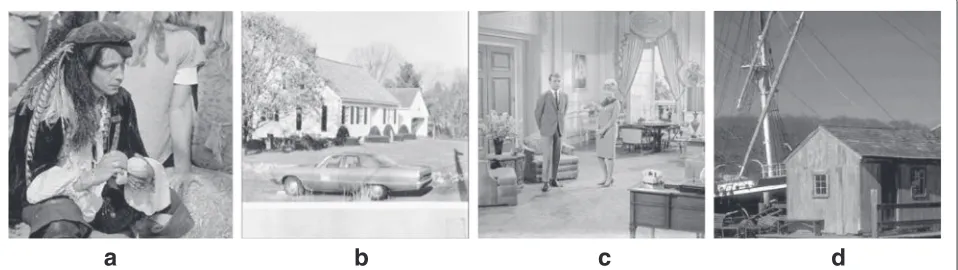
In this section, we compare all our algorithms with other methods. All the test images are shown in Fig. 5, one

1024×1024 image as (a) Man and three 512×512 images

as (b) Car, (c) Parlor, and (d) Housepole.

The quality of the restoration results is measured quan-titatively by using the peak signal-to-noise ratio (PSNR) in decibel (dB) and the relative error (ReE):

PSNR=10 log₁₀ n

2_Max2 I

f − ¯f2₂, ReE=

f − ¯f2 ¯f2 ,

where f¯ andf denote the original and restored images,

respectively, and MaxIrepresents the maximum possible

pixel value of the image. In our experiments, MaxI=1.

The stopping criterion used in our work is set to be as other methods

|Fk+1_−Fk_| |Fk_| <10

−5_{, (50)}

whereFk_{is the objective function value of the respective}

model in thekth iteration.

We compare our methods with some other methods, such as Chan et al.’s TV method proposed in [32], Liu et al.’s method proposed in [11], and Liu et al.’s method proposed in [12]. Both the latter two methods [11, 12] are with inner iteration MM methods for OGS TV problems, where the number of the inner iterations is set 5 by them. In particular, for a fair comparison, we set weighted matrix

Wg ∈ R3×3((Wg)i,j ≡ 1) in all the experiments of our

methods as in [11, 12].

5.3.1 Experiments for the constrained TV OGSL2model In this section, we compare our methods (CATVOGSL2 and CITVOGSL2) with some other methods, such as Chan et al.’s method proposed in [32] (Algorithm 1 in [32] for the constrained TV-L2 model) and Liu et al.’s method proposed in [11].

We set the penalty parameters β1 = 35, β2 =

20, for the ATV case, β1 = 100, β2 = 20 for the

ITV case and relax parameter γ = 1.618. The blur

kernels are generated by MATLAB built-in function (i)fspecial(’average’,9)for 9×9 average blur. We generate all blurring effects using the MATLAB built-in

functionimfilter(I,psf, ’circular’,’conv’)

under PBC with “I” as the original image and “psf” as

the blur kernel. We first generated the blurred images operating on images (a)–(c) by the former Gaussian blurs

a

b

c

d

Table 2Numerical comparison of Chan [32], Liu [11], CATVOGSL2, and CITVOGSL2 for images (a)–(c) in Fig. 5

Images (a) Man (b) Car (c) Parlor

Method _μ Itr PSNR Time ReE Itr PSNR Time ReE Itr PSNR Time ReE

Chan [32] 0.5 15 30.34 6.02 0.0730 11 31.13 2.00 0.0426 12 31.70 2.01 0.0511

Liu [11] 1 12 30.60 9.06 0.0708 12 31.68 3.93 0.0386 13 32.46 4.21 0.0464

CAOL2 1 7 30.62 3.37 0.0711 9 31.68 1.76 0.0399 7 32.40 1.34 0.0472

CIOL2 1 8 30.59 3.70 0.0716 11 31.60 2.04 0.0403 8 32.03 1.61 0.0492

PSNRdB,Times,Itriterations,μregularization parameter (×105_{),CAOL2CATVOGSL2,CIOL2CITVOGSL2}

and further corrupted by zero mean Gaussian noise with

BSNR=40. The BSNR is given by

BSNR=10 log₁₀ variance ofg

variance ofη.

where g and η are the observed image and the noise,

respectively.

The numerical results of the three methods are shown in Table 2. We have tuned the parameters for all the meth-ods as in Table 2. From Table 2, we can see that PSNR and ReE of our methods (both ATV and ITV cases) are almost

same as [11], which applied MM inner iterations to solve the subproblems (34) and (35) (only for the ATV case). However, each outer iteration of our methods is nearly twice faster than [11] from the experiments. The time of each outer iteration of our methods is almost the same as the traditional TV method in [32]. In Fig. 6, we display the restored “Parlor” images from different algorithms. We can see that OGS TV regularizers can get clearer edges on the “desk” of the image than TV regularizer.

Now, we compute the complexity of each step of our methods and Liu et al.’s method [11]. Firstly, we know that

the complexity of all the methods is 512×512×18×4

(4 times nlog₂n) except the OGS subproblems. Then,

for the OGS subproblems, the MM method in [11] with

five-step inner iteration, the complexity is 512×512×

90×2 (2 subproblems). The complexity of our methods is

512×512×18×2 in CATVOGSL2 and 512×512×18

in CITVOGSL2. Therefore, the total complexity of [11]

is 5122× 252, the total complexity of CATVOGSL2 is

5122×108, and the total complexity of CITVOGSL2 is

5122×90. That means each step of our methods is more

than double faster than the inner iteration method in [11]. In the next section, the common computation parts of our methods and the inner iteration method are much more, and then our methods are only nearly double faster.

Remarks 6.We do not list the results of image (d)

because they are almost the same as images (b) and (c).

Moreover, whenβ1 < 30 which is not sufficiently large,

the numerical results are also good while we did not list them. This shows that the approximate part of our shrink-age formula is also good, and that when the inner step in [11, 12] is chosen to be 5, the numerical experiments are convergent although they did not find a convergence control sequence. In addition, in our experiments, we find that the results of the ATV case are better than the ITV case, which is a little different from the classic TV meth-ods. Moreover, we find that if the parameters of [11] are

chosen to be the same as ours, the solutions of our method and their method are always the same on PSNR and visual presentation while our method may save more time (it remains valid for [12]).

5.3.2 Experiments for the constrained TV OGSL1model In this section, we compare our methods (CATVOGSL1 and CITVOGSL1) with some other methods, such as Chan et al.’s method proposed in [32] (Algorithm 2 in [32] for the constrained TV-L1 model) and Liu et al.’s method proposed in [12].

Similarly as the last section, we set the penalty

parame-tersβ1= 80,β2= 2000,β3 =1, for the ATV case,β1=

80,β2=2000,β3=1, for the ITV case and relax

param-eterγ = 1.618. The blur kernel is generated by

MAT-LAB built-in functionfspecial(’gaussian’,7,5)

for 7× 7 Gaussian blur with standard deviation 5. We

first generated the blurred images operating on images (b)–(d) by the former Gaussian blur and further cor-rupted them by salt-and-pepper noise from 30 to 40 %. We generate all noise effects by MATLAB built-in func-tionimnoise(Bl,’salt & pepper’,level)with

“Bl” the blurred image and fix the same random matrix

for different methods.

The numerical results by the three methods are shown in Table 3. We have tuned the parameters manually to give the best PSNR improvement for Chan [32] as in Table 3 for

Table 3Numerical comparison of Chan [32], Liu [12], CATVOGSL1, and CITVOGSL1 for images (a)–(d) in Fig. 5

Is N Chan [32] Liu [12]

L μ/Itr PSNR Time ReE Itr PSNR Time ReE

(a) 30 25/130 29.59 61.57 0.0796 35 30.92 30.23 0.0683

40 18/ 99 28.85 46.41 0.0866 37 30.11 31.54 0.0749

(b) 30 25/128 29.71 22.90 0.0501 35 31.81 12.93 0.0393

40 20/ 98 28.59 17.80 0.0570 40 30.70 14.99 0.0447

(c) 30 26/138 30.21 25.65 0.0607 35 32.15 12.84 0.0485

40 22/105 29.10 19.27 0.0689 37 31.04 13.67 0.0551

(d) 30 26/127 30.41 23.17 0.0975 36 32.47 13.15 0.0769

40 20/ 95 29.44 17.43 0.1091 39 31.43 14.27 0.0867

CATVOGSL1 CITVOGSL1

(a) 30 32 31.17 17.97 0.0663 41 31.34 21.56 0.0651

40 32 30.10 18.03 0.0751 37 30.06 19.95 0.0754

(b) 30 26 31.77 5.97 0.0395 29 31.75 6.26 0.0396

40 26 30.47 6.12 0.0459 29 30.22 6.38 0.0472

(c) 30 25 32.30 5.82 0.0477 30 32.08 6.75 0.0489

40 26 31.01 5.76 0.0553 27 30.50 6.19 0.0587

(d) 30 25 32.54 5.68 0.0764 29 32.51 6.75 0.0766

40 28 31.35 6.40 0.0875 32 31.06 7.33 0.0905

different images. For Liu [12], we choose the given

param-etersμdefault as 100, 80 for 30 and 40 %, respectively. For

our method CATVOGSL1, we setμas 180, 140 for 30 and

40 %, respectively. For our method CITVOGSL1, we set

μas 140, 100 for 30 and 40 %, respectively. In the

exper-iments, we find that the parameters of our methods are robust and have wide range to choose. Therefore, we set

the sameμfor different images.

From Table 3, we can also see that PSNR and ReE of our methods (both ATV and ITV cases) are almost the same as Liu [12], which applied MM inner iterations to solve the subproblems (34) and (35) (only for the ATV case). How-ever, each outer iteration of our methods is nearly twice faster than Liu [12] from the experiments. The time of each outer iteration of our methods is almost the same as the traditional TV method in Chan [32]. Moreover, we can also see that sometimes ATV is better than ITV and sometimes on the contrary for OGS TV. Finally, in Fig. 7, we display the degraded image, the original image, and the restored images for 30 % level of noise on image (d) by the four methods. From the figure, we can see that both our

methods and Liu [12] can get better edges (handrail and window) than Chan [32].

6 Conclusions

In this paper, we propose the explicit shrinkage formulas for one class of OGS regularization problems with trans-lation invariant overlapping groups. These formulas can be extended to several other regularization OGS prob-lems as a subproblem in many fields. In this work, we apply our results in OGS TV regularization problems— deblurring and denoising problems. Furthermore, we also extend the image deblurring problems with OGS ATV in [11, 12] to both ATV and ITV cases. Since the formulas are very simple, these results can be easily extended to many other applications such as multichannel deconvolu-tion and compress sensing, which we will consider in the future. In addition, in the experiments, we only choose all

the entries of the weight matrixWgequal to 1. We will test

for other weights in the future on more experiments in order to choose the better or best weights for some other applications.