doi:10.5194/ascmo-2-1-2016
© Author(s) 2016. CC Attribution 3.0 License.
Comparison of hidden and observed regime-switching
autoregressive models for (
u, v
)-components of wind
fields in the northeastern Atlantic
Julie Bessac1,2, Pierre Ailliot3, Julien Cattiaux4, and Valerie Monbet1,5
1Institut de Recherche Mathématiques de Rennes, UMR 6625, Université de Rennes 1, Rennes, France 2Mathematics and Computer Science Division, Argonne National Laboratory, Argonne, IL, USA 3Laboratoire de Mathématiques de Bretagne Atlantique, UMR 6205, Université de Brest, Brest, France
4CNRM-GAME, UMR 3589, CNRS/Météo France, Toulouse, France 5INRIA Rennes, ASPI, Rennes, France
Correspondence to: Julie Bessac ([email protected])
Received: 18 August 2015 – Revised: 23 December 2015 – Accepted: 10 February 2016 – Published: 29 February 2016
Abstract. Several multi-site stochastic generators of zonal and meridional components of wind are proposed in this paper. A regime-switching framework is introduced to account for the alternation of intensity and variability that is observed in wind conditions due to the existence of different weather types. This modeling blocks time series into periods in which the series is described by a single model. The regime-switching is modeled by a discrete variable that can be introduced as a latent (or hidden) variable or as an observed variable. In the latter case a clustering algorithm is used before fitting the model to extract the regime. Conditional on the regimes, the observed wind conditions are assumed to evolve as a linear Gaussian vector autoregressive (VAR) model. Various questions are explored, such as the modeling of the regime in a multi-site context, the extraction of relevant clusterings from extra variables or from the local wind data, and the link between weather types extracted from wind data and large-scale weather regimes derived from a descriptor of the atmospheric circulation. We also discuss the relative advantages of hidden and observed regime-switching models. For artificial stochastic generation of wind sequences, we show that the proposed models reproduce the average space–time motions of wind conditions, and we highlight the advantage of regime-switching models in reproducing the alternation of intensity and variability in wind conditions.
1 Introduction
In this section, we present the context of our work and then the data used to compare the proposed Markov-switching au-toregressive models.
Stochastic weather generators have been used to generate artificial sequences of small-scale meteorological data with statistical properties similar to the data set used for cali-bration. Various wind condition generators at a single site have been proposed in the literature; see Brown et al. (1984), Flecher et al. (2010), and Ailliot and Monbet (2012). How-ever, few models have been introduced in a multi-site con-text (Haslett and Raftery, 1989; Bessac et al., 2015). Arti-ficial sequences of wind conditions provided by stochastic
weather generators enable assessment risks in impact stud-ies; see, for instance, Hofmann and Sperstad (2013). Here we propose a multi-site generator for Cartesian components of surface wind. As far as we know, only a few models have been proposed to simulate time series of Cartesian coordi-nates of wind{ut, vt}(Hering et al., 2015; Hering and
Gen-ton, 2010; Ailliot et al., 2006; Wikle et al., 2001; Fuentes et al., 2005). Except in Hering et al. (2015), these models are designed for short-term wind prediction and not for the generation of artificial conditions of{ut, vt}. Consequently
they are not focused on reproducing the same statistics we are interested in, namely, the marginal distribution of{ut, vt}
is proposed. The proposed Markov-switching vector autore-gressive model enables reproduction of many spatial and temporal features; however, complex dependencies between intensity and direction remain hard to model.
In the northeastern Atlantic, the spatiotemporal dynam-ics of the wind field is complex. This area is under the in-fluence of an unstable atmospheric jet stream whose large-scale fluctuations induce local alternations between periods with high wind intensity and strong temporal variability, and less intense and variable periods. Scientists have pro-posed describing the North Atlantic atmospheric dynamics through a finite number of preferred states, namely, weather regimes or weather types (Vautard, 1990). However, intro-ducing regime-switching in the modeling of local wind, as we propose in this paper, enables us to better reproduce the spatiotemporal characteristics observed in the wind data. In practice, describing a time series by regimes involves a par-titioning into time periods in which the series is homoge-neous and can be described by a single model. In this pa-per, we propose various vector autoregressive (VAR) models with regime-switching. One of the challenges is to achieve a regime-switching that is physically consistent and that en-ables appropriate describing of the local observation by a VAR model. To this end, we introduce several frameworks of regime-switching and compare them in terms of simula-tion of wind data.
Depending on the availability of good descriptors of the current weather state, regime-switching can be introduced with either observed or latent regimes. Regimes are said to be observed when they are identified a priori, before the model-ing of the local dynamics. In this case, clustermodel-ing methods are run on adequate variables to obtain relevant regimes: either the local variables or extra variables characterizing the large-scale weather situation, such as descriptors of the large-large-scale atmospheric circulation (Bardossy and Plate, 1992; Wilson et al., 1992) or variables enabling the separation into dry and wet states (Richardson, 1981; Flecher et al., 2010). For wind models, the wind direction can be considered since it is a good descriptor of synoptic conditions. In Gneiting et al. (2006), the wind direction is used both to extract regimes and to parameterize of the predictive distribution. In this paper, we propose a priori clusterings based on both large-scale and local variables.
When the regimes are said to be latent, they are intro-duced as a hidden variable in the model. This framework is more complex from a statistical point of view and the con-ditional distribution of wind given that the regime has to be simple and tractable. Hidden Markov models (HMMs) have been widely used for meteorological data (Zucchini and Gut-torp, 1991; Hughes et al., 1999; Thompson et al., 2007). Hidden Markov-switching autoregressive (MS-AR) models are a generalization of HMMs allowing temporal dynamics within the regimes (Hamilton, 1989). Models with regime-switching improve the modeling of wind intensity time se-ries with classical autoregressive–moving-average (ARMA)
models; see Ailliot and Monbet (2012), where the wind speed is modeled at one site. Here we propose a hidden MS-AR model and compare it with several models with observed regime-switching.
To the best of our knowledge, no comparison between ob-served and latent regime-switching has been proposed in the field of stochastic generators of wind conditions. In Pinson et al. (2008), a comparison is presented in terms of wind prediction between models with hidden regimes and models driven by observed regimes. In this work, we compare both kinds of models in a simulation framework.
In the multi-site context, the regime can either be common to all sites (i.e., scalar; see Ailliot et al., 2009) or introduced as a site-specific regime (Wilks, 1998; Kleiber et al., 2012; Khalili et al., 2007; Thompson et al., 2007), which enables one to account for a wide range of space–time dependencies. However, a site-specific regime appears to be computation-ally challenging (Wilks, 1998). We will show that the choice of a regional regime is reasonable when a homogeneous area is selected.
The paper is organized as follows. MS-AR models are in-troduced in Sect. 3, and their inference is described in cases of both observed and latent regime-switching. The question of a regional regime is addressed in Sect. 4. In Sect. 5, we in-troduce and discuss different sets of a priori regimes obtained by clustering. In Sects. 7 and 8, respectively, we discuss the advantages of the proposed models and highlight the differ-ences between observed and latent regime-switching models.
2 Wind data
The data under study are zonal (west–east) and merid-ional (north–south) surface wind components {ut, vt} at
10 m a.s.l. (above sea level) extracted from the ERA-Interim data set produced by the European Centre for Medium-Range Weather Forecasts (ECMWF). It can be freely downloaded from the url http://apps.ecmwf.int/datasets/data/ interim-full-daily/ and used for scientific purposes.
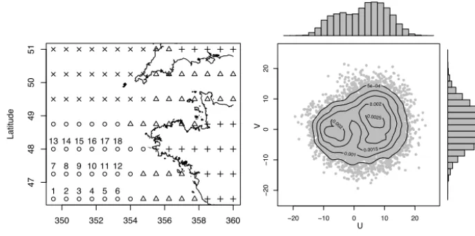
350 352 354 356 358 360 47 48 49 50 51 Longitude Latitude
1 2 3 4 5 6 7 8 9 10 11 12 13 14 15 16 17 18
−20 −10 0 10 20
− 20 − 10 0 1 0 2 0
5e−04
0.001 0.0015 0.002 0.002 0.0025 U V
Figure 1.Left: spatial hierarchical clustering of the moving variance associated with wind speed with four clusters (symbols). Right: joint and marginal distribution of{ut, vt}at the central location 10; contour lines of the estimated joint density.
which is described more precisely in Sect. 7. This process is a good descriptor of the temporal characteristics of wind time series (see Fig. 4), and it is computed as the standard de-viation of wind speed over nine consecutive time steps (i.e., 2 days). The dendogram associated with the clustering sug-gests the use of four clusters that are depicted in Fig. 1. These four clusters are likely to be divided into an inland cluster (+), an intermediate cluster between ocean and land (4), a cluster corresponding to flows that propagate into the Bay of Biscay (◦), and a cluster for flows that propagate toward northern Europe (×).
Components{ut}and{vt}show a complex relationship, as
partially reflected by the joint distribution of{ut, vt}(Fig. 1).
The margin of{ut}reveals two separate modes, whereas that
of{vt}does not exhibit a clear bimodality. The contour lines
show that the density is low around the point (0,0). It in-dicates that the transitions between the two modes of each component are not realized through a vanishing of the field, but rather through a rotation of the field. The following trans-formation is used on both components {ut}and {vt}. This
transformation withα >1 facilitates the modeling of the bi-modality:
(
eut= U
α
t cos(8t),
evt= U
α
t sin(8t),
(1)
where {Ut}and{8t}, respectively, denote wind speed and
wind direction. In practice,αis chosen empirically equal to 1.5. This transformation has proven helpful in modeling the distribution of{ut, vt}in Ailliot et al. (2015).
3 Markov-switching vector autoregressive models
In this section, we introduce the proposed models and discuss their parameter estimation in cases of both observed and la-tent regimes.
3.1 The models
In this paper, we consider the following class of models. Let St be a discrete Markov chain with values in{1, . . ., M}
de-scribing the current weather type as a function of timet. Con-ditional on the weather type, the observed wind conditions are modeled as a vector autoregressive model. Given the cur-rent value ofSt, the observationYt is written as
Yt=A(0St)+A(1St)Yt−1+A(2St)Yt−2+. . .+A(pSt)Yt−p
+(6(St))−1/2t. (2)
Y∈R2K represents the observed power-transformed wind
components {ut, vt} at the K locations, given by the
sys-tem (Eq. 1). For i∈ {1, . . ., M}, A(0i) is a 2K-dimensional vector, A(1i), . . .,Ap(i),6(i) are 2K×2K matrices, and
is a Gaussian white noise of dimension 2K. Conditional independencies between S and Y are displayed on the following directed acyclic graph (DAG) for p=1 (see Durand, 2003, for additional information about DAGs).
mation is used on both components{ut}and{vt}. This transformation withα >1facilitates the modeling of the bimodality:
115
˜
ut= Utαcos(Φt) ˜
vt= Utαsin(Φt),
(1)
where{Ut}and{Φt}respectively denote wind speed and wind direction. In practice,αis chosen empirically equal to1.5. This transformation has proven helpful in modeling the distribution of {ut, vt}in (Ailliot, Bessac, Monbet, and Pene, 2015).
2 Markov-switching vector autoregressive models
120
In this section, we introduce the proposed models and discuss their parameter estimation in cases of
both observed and latent regimes.
2.1 The models
In this paper, we consider the following class of models. LetStbe a discrete Markov chain with values in{1, ..., M}describing the current weather type as a function of timet. Conditionally to the
125
weather type, the observed wind conditions are modeled as a vector autoregressive model. Given the
current value ofSt, the observationYtis written as
Yt=A(0St)+A (St)
1 Yt−1+A2(St)Yt−2+...+Ap(St)Yt−p+ (Σ(St))−1/2t. (2)
Y ∈R2K represents the observed power-transformed wind components{u
t, vt}at theKlocations, given by the system (1). For i∈ {1, ..., M},A(0i) is a2K-dimensional vector,A(1i), ...,A(pi),Σ(i) 130
are2K×2K-matrices, andis a Gaussian white noise of dimension2K. Conditional independen-cies betweenS andY are displayed on the following directed acyclic graph (DAG) forp= 1(see (Durand, 2003) for additional information about DAGs):
··· //
St−1 //
St //
St+1 //
···
··· //Yt−1 //Yt //Yt+1 //···
In this model, the regime S can be latent or observed; both cases are discussed, respectively, in
135
Sections 3 and 4. The parameter estimation of the model can be performed by maximum likelihood
but in a different way in each framework.
For both kind of models, covariates can be included. The easiest way is to include them in the
intercept parameter A0 or in transitions between regimes. Transitions between regimes can be
parametrized with a covariate (when regimes are latent, a parameterization with an extra
covari-140
ate is given in (Hughes and Guttorp, 1994) and with the studied variable in (Ailliot, Bessac, Monbet,
5
In this model, the regimeS can be latent or observed; both cases are discussed, respectively, in Sects. 4 and 5. The pa-rameter estimation of the model can be performed by maxi-mum likelihood but in a different way in each framework.
For both kinds of models, covariates can be included. The easiest way is to include them in the intercept parameter A0 or in transitions between regimes. Transitions between
are defined a priori). In the context of multi-site models, the choice of the covariate of non-homogeneous transitions is delicate. We do not discuss this topic here and consider only homogeneous transition models.
To avoid over-parameterization of the conditional models, we first work with a reduced data set. In the following, all the proposed models will be fitted on the subset of sites (1, 6, 10, 13, 18), the extension to a wider region being left for future studies.
3.2 Estimation by maximum likelihood
First, let us suppose that the complete set of observa-tions (y1, . . .yT, s1, . . . sT) is available, which is the case in
Sect. 5. Assume thats0,y−1, andy0are observed. Then the
complete log-likelihood, associated with an autoregressive orderp=2 (we choosep=2 according to a previous work – Ailliot et al., 2015), is written as
log(L(θ;y1, . . .yT, s1, . . . sT|y−1,y0, s0))
=log(L(θ(Y);y1T|y−1,y0, s0T))
+log(L(θ(S);s1T|y−1,y0, s0)), (3)
whereθ=(θ(S),θ(Y)).θ(Y)corresponds to the parameters of the VAR models, θ(S)=5=(πi,j)i,j=1,···,M the transition
matrix 5 of the Markov chain S, and yT
1 =(y1, . . . ,yT).
Let us denote ni,j the number of occurrences of the event
{(St, St+1)=(i, j)} for t∈ {1, . . . , T−1}, ni,.=PMj=1ni,j
andni=ni,.+δ{sT=i}, whereδis the Kronecker symbol, the
total number of occurrences of the regimei:
log(L(θ(Y);y1, . . .,yT|y−1,y0, s0T))
=
T
X
t=1
log(p(yt|yt−1,yt−2, st))
=
M
X
i=1
X
t∈{t|st=i}
log(p(yt|yt−1,yt−2, st))
=
M
X
i=1
ni(−
d
2log(2π)− 1
2log(det(6
(i)))
− X
t∈{t|st=i} 1 2e
0
t(6
(i))−1e
t,
whereet=(yt−A
(i) 0 −A
(i)
1 yt−1−A (i) 2 yt−2).
For eachi∈ {1, . . . , M}, each function
θ(Y,i) → ni(−
d
2log(2π)− 1
2log(det(6
(i)))
− X
t∈{t|st=i} 1 2e
0
t(6
(i))−1e
t
can be maximized separately, where θ(Y,i)= (A(0i),A(1i),A2(i),6(i)). The optimal estimates of A1(i)and A(2i)
are computed by writing the VAR(2) model as VAR(1): for allt∈ {t|st=i},
Yt
Yt−1
=
A(1i) A(2i) IdK 0
Yt−1
Yt−2
+ t 0 ,
where IdKis theK×K-identity matrix. Let us write
A(i)=
A(1i) A(2i) IdK 0
and
Zt =
Yt
Yt−1
;
expressions ofAˆ(1i)andAˆ(2i)are extracted from the estimate
ˆ
A(i)= X
t∈{t|st=i} ZtZ0t−1
X
t∈{t|st=i}
Zt−1Z0t−1
−1
. (4)
The other optimal estimates are
ˆ
A(0i)=(IdK− ˆA(1i)− ˆA (i) 2 )µˆ
(i), (5)
whereµˆ(i)= 1 ni
X
t∈{t|st=i}
yt is the empirical mean ofYin
regimeiand
ˆ 6(i)= 1
ni
X
t∈{t|st=i} ˆ
eteˆ0t. (6)
ˆ
6(i) is the empirical variance of the empirical residuals de-fined aseˆt=(yt− ˆA
(i) 0 − ˆA
(i)
1 yt−1− ˆA (i) 2 yt−2).
Concerning the Markov chainS,
log(L(θ(S);s1, . . . , sT|y−1,y0, s0))=
M
X
i,j=1
ni,jlog(πi,j),
the associated maximum likelihood estimator is
ˆ πi,j =
ni,j
ni,.
.
When observations only of processYare available and the realizations ofS are not given a priori, as in Sect. 4, one in-ference method is to use the expectation–maximization (EM) algorithm, which is commonly run to estimate the parame-ters of models with latent variables by maximum likelihood. SinceSis not observed, the EM algorithm aims at maximiz-ing the incomplete log-likelihood function based on the ob-servationsY:
θ→Eθ(log(L(θ;Y1, . . . ,YT, S1, . . . , ST))|YT−1
=yT−1, S0=s0).
The EM algorithm cycles through two steps: the expec-tation step and the maximization step (Wu, 1983; Demp-ster et al., 1977). The E step is performed through forward– backward recursions (see Hamilton, 1990 for hidden MS-AR models) that enable one to compute the smoothing probabil-itiesP(St|YT−1=yT−1, S0=s0). At the M step, optimal
ex-pressions of parameters ofθ(Y), given in Eqs. (4), (5), and (6), are used. In each regime i, however, each observationyt is weighted by the probabilityP(St=i|YT−1=yT−1, S0=s0),
for instance,
ˆ
µ(i)= 1
PT
t=1P(St=i|YT−1=yT−1, S0=s0)
T
X
t=1
P(St=i|YT−1=y
T
−1, S0=s0)yt. (7)
The transition matrix is estimated from quantities P({St=
i, St+1=j}|YT−1=yT−1, S0=s0) that are derived at the E
step.
In this paper, we use AP-MS-VARC to denote the a
pri-ori regime-switching model associated with the clustering C, and we use H-MS-VAR to denote the hidden regime-switching model.
4 Regime definition in a multi-site context
When the current weather state is not estimated a priori, it is introduced as a latent variable. Hidden regime-switching models have been used in various fields; see Zucchini and MacDonald (2009) for a wide range of applications of hid-den Markov models. In a previous work (Ailliot et al., 2015) a single-site model for {ut, vt}was proposed; the proposed
hidden Markov-switching autoregressive model reveals good qualities to describe both marginal and joint distributions of {ut, vt}as well as the temporal dynamics of the wind at one
location. In this paper we propose an extension of this model, when the process{ut, vt}is multi-site. In a multi-site context,
the regime can be site-specific or common to all stations. Here, the assumption of a common regional regime is investigated, and we show that this assumption is accept-able when the considered area is homogeneous. The ho-mogeneous single-site MS-AR model introduced in Ailliot et al. (2015) for{ut, vt}withM=3 regimes and an
autore-gressive order p=2 has been fitted at each site. The most likely regimes associated with the data are extracted from the estimation procedure of H-MS-VAR models described in the previous section. At each time, the regime corresponds to arg maxj∈{1,···,M}P(St=j|YT−1=y
T
−1, S0=s0); see
Zuc-chini and MacDonald (2009). In order to properly compare the regimes, they are ordered according to the increasing value of the determinant of the matrix 6(i). The intuition for sorting regimes according the determinant of6(i)is that we expect the innovations to be more volatile, and conse-quently6(i)to have greater eigenvalues, in cyclonic weather
regimes. Conversely, we expect to observe innovations more persistent in time in calm weather regimes; this is associated with smaller eigenvalues of6(i). The spatiotemporal coher-ence of the regimes of each of the 18 sites is checked and reveals a strong homogeneity that motivates the use of a re-gional regime in this area.
The sequences of regimes are compared in Fig. 2; time se-ries of a posteriori regimes and wind speed are depicted. The last two regimes are less coherent from one site to another. This effect is partly explained by the fact that these regimes are less persistent in time, especially the third one (see Ta-ble 1).
Moreover, we can notice an eastward propagation in wind events, the darkest regimes often being observed at western stations (station 1) prior to eastern sites (10 and 18). The bot-tom panel of Fig. 2, which depicts the sequences of regimes associated with the model fitted on the set of all locations with a regime common to all locations, reveals that this re-gional regime is coherent with the local ones, although it is less persistent. Indeed, when fitting the model to several sta-tions, the regime has to embed some spatial heterogeneity that is likely to decrease the temporal persistence.
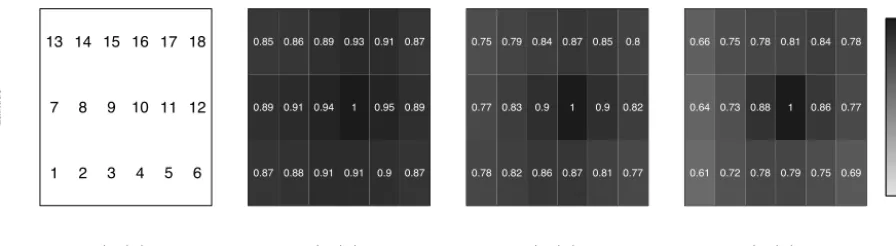
In Fig. 3, probabilities of occurrence of a given regime conditional on the simultaneous occurrence of the same regime at site 10 are depicted for all sites. In each picture, conditional probabilities should be compared with the refer-ence value given at location 10, which is 1 by construction. The first regime has the best spatial coherence, and the third regime, which is the least persistent regime, is less coherent spatially. The ranges of values of these probabilities indicate a satisfying consistency between the regimes across sites.
At each site, the physical interpretation of each regime is similar. Indeed, the first regime corresponds mainly to anti-cyclonic conditions with easterly winds and a slowly varying intensity (the variance of the innovation of the AR model is lower than in the two other regimes, and the first AR coeffi-cient is larger; see Table 1).
The two other regimes correspond to cyclonic conditions with westerly winds and a higher temporal variability in the intensity (see Fig. 4). These two regimes are discrim-inated mainly by the temporal variability, which is higher in the third regime. Moreover, the wind direction, not de-picted here, slightly differs: from southwesterlies in the sec-ond regime to northwesterlies in the third regime.
Longitude
Latitude
1 2 3 4 5 6
7 8 9 10 11 12
13 14 15 16 17 18
Longitude
0.87 0.88 0.91 0.91 0.9 0.87
0.89 0.91 0.94 1 0.95 0.89
0.85 0.86 0.89 0.93 0.91 0.87
Longitude
0.78 0.82 0.86 0.87 0.81 0.77
0.77 0.83 0.9 1 0.9 0.82
0.75 0.79 0.84 0.87 0.85 0.8
Longitude
0.0 0.2 0.4 0.6 0.8 1.0
0.61 0.72 0.78 0.79 0.75 0.69
0.64 0.73 0.88 1 0.86 0.77
0.66 0.75 0.78 0.81 0.84 0.78
Figure 3.Leftmost panel: matrix with the number of the station is printed; then, from left to right, conditional probabilities of occurrence of regimei=1,2,3 at all sites conditional on the simultaneous occurrence of the same regime at site 10; in each pixel, the value of the conditional probability is plotted.
Coefficients of the autoregressive process Y in each regime and the transition matrix at each site are compara-ble and spatially coherent (see Tacompara-ble 1). Other criteria such as the average field of{ut, vt}in each regime and the
distri-bution of{8t}in each regime were also explored and suggest
similarities between regimes at all locations.
The assumption of a regional regime seems appropriate in the considered area and is thus kept for the modeling of the multi-site wind in the following.
5 Observed regime-switching autoregressive models
Conversely to the previous section, one may derive the regimes separately from the fitting of the conditional model. For such a priori regime-switching models, the derivation of observed regimes can be done with appropriate cluster-ing methods. We seek weather states that are distinct from one other and in which the data are homogeneous. Cluster-ing can be run either on the local variables under study or on extra variables: the former leads to weather states that are more appropriate to the local data, while the latter can pro-vide more meteorologically consistent regimes, for example, with more information about the large-scale situation. In this subsection, we propose three clusterings, which differ by the clustering method and/or by the variables used to derive the a priori regimes.
5.1 Derivation of observed regimes from extra variables: CZ500
As a first clustering, we use a classification into four large-scale weather regimes that is commonly used in climate studies to characterize the wintertime atmospheric dynamics over the North Atlantic/European sector (Michelangeli et al., 1995; Cassou, 2008; Najac, 2008). These regimes can be de-scribed as follows.
– The positive phase of the North Atlantic Oscillation (hereafter NAO+), characterized by a strengthening of
both the Azores High and the Islandic Low, which rein-forces the westerlies.
– The negative phase of the NAO (NAO−), its symmetri-cal counterpart
– The Scandinavian blocking (BL), characterized by a strong anticyclone over northern Europe able to totally block the westerly flow over western Europe
– The Atlantic Ridge (AR), characterized by a strong west–east pressure dipole bringing polar air masses over western Europe
At the local scale of our area of study, these regimes are, respectively, associated with strong southwesterly flows (NAO+), weak westerly flows (NAO−), stable southerly or easterly flows (BL), and northerly flows (AR).
Table 1.Parameter values obtained when fitting a H-MS-VAR at the different sites: diagonal of the transition matrix5, coefficients of the autoregressive model in each regime, and logarithm of the determinant of6(i).
Diagonal of5 AR coefficients (A(1i)(1,1),A1(i)(2,2)) log(det(6(i)))
Site/regime R1 R2 R3 R1 R2 R3 R1 R2 R3
Site 1 0.93 0.83 0.64 (1.27, 1.16) (1.15, 1.3) (0.62, 0.63) 5.62 8.87 11.96 Site 6 0.92 0.83 0.71 (1.27, 1.02) (1.2, 1.28) (0.61, 0.72) 5.55 8.59 11.79 Site 10 0.93 0.84 0.74 (1.25, 1.19) (1.17, 1.27) (0.74, 0.71) 5.55 8.67 11.79 Site 13 0.93 0.81 0.64 (1.22, 1.24) (1.17, 1.25) (0.65, 0.65) 5.77 9 11.96 Site 18 0.93 0.83 0.73 (1.26, 1.12) (1.17, 1.25) (0.67, 0.68) 5.72 8.73 11.83
0
5
10
15
20
25
Moving mean
0
5
10
15
20
25
Moving mean
0
5
10
15
20
25
Moving mean
02468
Moving standard deviation
02468
Moving standard deviation
02468
Moving standard deviation
R1 R2 R3
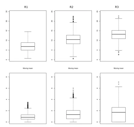
Figure 4.Top panel: moving mean of wind speed computed on 2-day intervals (nine time steps) for each regime of the H-MS-VAR model
5.2 Derivation of observed regimes from the local variables: CEOF(u,v)and CDiff(u,v)
To derive observed regimes from local wind variables, one can first use a k-means clustering procedure similar to the one used for CZ500. However, while CZ500provides
persis-tent regimes in which the conditional model satisfyingly de-scribes{ut, vt}, local regimes resulting from such ak-means
clustering are not persistent enough to reliably estimate the conditional VAR model. Consequently, in this subsection, we perform the local clustering via a hidden Markov model with Gaussian probability of emission.
The hidden structure of the Markov chain provides more stable regimes than with ak-means clustering. It corresponds to an H-MS-VAR model with VAR models of order p=0. The EM algorithm is used to process the clustering, and the number of regimes is chosen to be 3. This number provides the most physically relevant local regimes; a greater num-ber of regimes indeed leads to less discriminative regimes in terms of local wind conditions (not shown).
Then two sets of descriptors of the data (i.e., local vari-ables) are proposed. The first partition, denoted CEOF(u,v),
is obtained by clustering the time series associated with the first two EOFs of the anomalies of {ut, vt}, which explain
94% of the total variance. The second partition involves de-scriptors of the conditional distribution ofp(Yt|Yt−1), in
or-der to find a clustering that may be better adapted to the de-scription of the conditional distribution by an autoregressive model. A simplified way to describe the dynamics is to con-sider the bivariate process{ut−ut−1, vt−vt−1}. This set of
variables enables construction of regimes that discriminate well the temporal variability of the process{ut, vt}. Let us
denote this second local clustering as CDiff(u,v).
6 Analysis of the proposed clusterings
The proposed clusterings are compared through various anal-yses. We seek a clustering that is physically meaningful and appropriate in terms of conditional autoregressive models. For a proper comparison, for all clusterings, we decide to order regimes from the more persistent to the less persistent. This is done according to the determinant of the matrix6(i).
6.1 First visual comparison
Sequences of regimes from the proposed clusterings are shown in Fig. 5. The top panel shows that CZ500 has very
persistent regimes. This result is expected because it de-scribes the alternation between the preferred states of the large-scale atmospheric dynamics, whose typical timescale is a few days. One can see that the less volatile wind con-ditions are associated with the BL and AR phases, whereas the most variable wind conditions occur during the two NAO phases; see Fig. 10. The three bottom panels correspond to local clusterings. For all of them, the first regime is
associ-ated with the less volatile conditions with weakest intensity, whereas the second and third regimes are generally associ-ated with moderate and high intensities of wind. However, the behavior of the regime-switching differs from one clus-tering to another, probably because of the different choice of descriptors ({ut, vt}vs.{ut−ut−1, vt−vt−1}) and/or methods
(observed vs. latent) used in the clustering. The bottom panel of Fig. 2 shows that the second regime is a precursor to the third one (which is confirmed by the transition probabilities between regimes), and that this second regime is associated most of the time with rises in wind speed intensity.
In Fig. 6, the average fields corresponding to each regime of the four clusterings are plotted. The top row highlights the difficulty of discriminating local wind features when us-ing regimes defined from a large-scale circulation variable. While the AR and NAO+regimes of CZ500 are associated
with strong local wind signatures (as described in Sect. 5.1), the BL and NAO−regimes have a weaker discriminatory power in the local wind data. This issue was also observed in Najac (2008).
Since different descriptors are used, CDiff(u,v) and
CEOF(u,v)lead to very different results. CEOF(u,v)leads to the
most physically consistent regimes: a northeasterly regime, a northwesterly one, and a southwesterly one, which are flows corresponding to several of the large-scale weather regimes. The last two regimes are associated with stronger intensities. From the derivation of this clustering, one naturally finds regimes that correspond to the main mean patterns of vari-ability of the fields.
The regimes of CDiff(u,v)have less persistence, which
com-plicates their meteorological interpretation. The first regime corresponds to periods of weak wind intensities. The last two regimes are southwesterly regimes with a different in-tensity from one to the other. The averaged fields of the regimes extracted from H-MS-VAR are similar to the ones of CDiff(u,v) despite some punctual discrepancies in their time
series (Fig. 5). The first regime of these two clusterings seems associated with blocking situations.
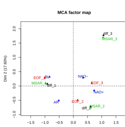
To compare the associations between the different classifi-cations, a multiple correspondence analysis is made between the four categorical variables that represent each classifica-tion. This analysis can be viewed as an analog of a principal component analysis for categorical variables where the as-sociations between the variables are measured with the Chi-squared distance. The regimes of each classification are pro-jected on the first two components and displayed in Fig. 7. These two axes enable one to account for 44 % of the vari-ance, which is not low for such an analysis. The other axes are not considered because they do not bring enough use-ful information. Note that this analysis does not account for the temporal dependence in each classification. The overall structure tends to associate the three classifications CEOF(u,v),
CDiff(u,v), and H-MS-VAR, except for the third regime of
CEOF(u,v). The classifications CDiff(u,v)and H-MS-VAR are
Figure 5.Time series of wind speed in January 2012 and a priori regimes extracted from the proposed methods above. The darker is the grey; the smaller is the determinant of6(i). From top to bottom: CZ500, CEOF(u,v), CDiff(u,v), and regimes from the fitting of the H-MS-VAR
model.
mainly occur at the same time, and this coincides with Fig. 5. The first axis contrasts time-persistent regimes with less per-sistent ones. Regime BL is close to regimes R1 of CEOF(u,v),
CDiff(u,v), and H-MS-VAR; this is also seen in Table 3 and
is in agreement with the average fields of these regimes dis-played in Fig. 6. The second axis contrasts regimes R2 of H-MS-VAR and CDiff(u,v)with regimes R3, which is also a
contrast between persistent and less persistent regimes. Most of these similarities between the regimes are also seen in Table 2 through the logarithm of the covariance of the in-novations and the percentage of time spent in each regime. Regime AR from CZ500 seems more difficult to associate
Figure 6.Average fields of{ut, vt}in each regime of the clusterings, from top to bottom: CZ500, CEOF(u,v), CDiff(u,v), and from the fitting
of H-MS-VAR on the set of five locations.
with weather regime NAO+, which coincides with Table 3 and Fig. 6.
6.2 Quantitative analyzing
Quantitative criteria are considered in order to complete this analysis. The optimal value of the complete log-likelihood
of the model is generally a good measure of the statistical relevance of a model. The complete log-likelihood, given in Eq. (3), evaluated at the maximum likelihood estimator of ˆ
Table 2.Npis the number of parameters. Values are computed from models fitted on{ut, vt}at the five locations (1, 6, 10, 13, 18).
BIC log-L log-L Np log(det(6(i))) % of time spent
Model ofS ofY R1 R2 R3 R4 R1 R2 R3 R4
Unconditional VAR 542 640 – −269 825 265 36.4 – – – – – – –
AP-MS-VARCZ500 542 730 −1510 −263 808 1072 29.8 30.3 39 38.1 0.27 0.18 0.2 0.34
AP-MS-VARCEOF(u,v) 545 730 −2331 −266 015 801 28.9 33.3 38.9 – 0.31 0.42 0.27 – AP-MS-VARCDiff(u,v) 520 759 −4762 −251 099 801 20.2 34.1 48.1 – 0.44 0.41 0.15 –
H-MS-VAR 459 458 – −229 616 801 18.4 32.1 48.4 – 0.43 0.41 0.16 –
−1.5 −1.0 −0.5 0.0 0.5 1.0 1.5
−1.0
−0.5
0.0
0.5
1.0
1.5
2.0
MCA factor map
Dim 1 (26.34%)
Dim 2 (17.60%)
diff_1
diff_2
diff_3
EOF_1
EOF_2 EOF_3 MSAR_1
MSAR_2 MSAR_3
AR
BL NAO−
NAO+
Figure 7.First plan of the multiple correspondence analysis made of the four classifications. Each regime of the four classifications is depicted.
sum of the following two terms:
log(L(θˆ(Y);yT1|s1T))= −T dlog(2π)
2 −
T d 2
−
M
X
i=1
nilog(det(6ˆ(i)))
and
log(L(θˆ(S);s1, . . . , sT))= M
X
i,j=1
ni,jlog
ni,j
ni,.
.
Note that the first term is a function of the total time spent in each regime and the associated determinant of covariance matrix of innovation (note that the one-step-ahead error of the forecast is linked to this quantity). The longer the time spent in a regime with a weak determinant of covariance of innovation, the greater the log-likelihood (see Table 2). The maximal log-likelihood of θ(S) is equal to the opposite of the conditional entropy of St given St−1. The conditional
entropy is classically used as a quality measure of cluster-ing. In prediction, the weaker the entropy, the stronger the predictability ofSt givenSt−1. More generally one tends to
minimize this measure. Because of the range of values of the log-likelihood ofθ(Y), the value of that ofθ(S)has a low contribution to the complete log-likelihood. If the complete log-likelihood is used to select models, the persistence of the Markov chain has a low impact. BIC indexes are also given in Table 2, where BIC= −2 log L+Nplog(Nobs), with L the
likelihood of the model, Np the number of parameters and
Nobsthe number of observations. The BIC index enables one
to consider a compromise between a model with a high like-lihood and its parsimony. Note that one should not compare BIC indexes of a priori and latent regime-switching models. However, the BIC indexes of these two classes of models can be compared with that of the unconditional VAR model, since it is a particular case.
The clustering CDiff(u,v) provides the greatest value of
complete log-likelihood. The lower value of log-likelihood ofS, with shorter persistence in the different regimes com-pared with the other models, is compensated for by a larger value of log-likelihood of Y and thus a longer time spent in regimes with low variances of innovation. The three pro-posed AP-MS-VAR models lead to a satisfying description of the marginal and joint distributions and space–time covari-ances (not shown). The model AP-MS-VARCDiff(u,v), which
exhibits the best likelihood, performs the most accurately among the AP-MS-VAR models to reproduce the moving av-erage and moving variance processes; see Sect. 7. Besides, in terms of BIC indexes, the smallest value among the AP-MS-VAR models is that of AP-MS-AP-MS-VARCDiff(u,v), and it is also
greater than that of the VAR model. In the following, the VAR model with shifts defined by CDiff(u,v)is kept for
fur-ther comparisons with the H-MS-VAR model in simulation; see Sect. 7. We choose this model although it is not the most physically meaningful because it leads to better results ac-cording to our criterion.
6.3 Link between large-scale weather regimes and local ones
Table 3.Joint probability of occurrence of the three local regimes identified by the proposed models in rows and the four large-scale regimes in columns.
CEOF(u,v) CDiff(u,v) H-MS-VAR
BL AR NAO− NAO+ Total BL AR NAO− NAO+ Total BL AR NAO− NAO+ Total
R1 0.17 0.06 0.08 0.01 0.32 0.15 0.10 0.07 0.13 0.45 0.13 0.09 0.07 0.14 0.43
R2 0.04 0.10 0.05 0.08 0.27 0.09 0.06 0.09 0.16 0.40 0.10 0.06 0.09 0.15 0.41
R3 0.07 0.02 0.07 0.26 0.42 0.03 0.02 0.04 0.06 0.15 0.04 0.02 0.05 0.06 0.16
Total 0.28 0.18 0.20 0.35 1 0.27 0.18 0.20 0.35 1 0.27 0.17 0.21 0.35 1
−20 −10 0 10 20
−
20
−
10
0
1
0
2
0
5e−04
0.001 0.001
0.0015
0.002
0.0025
U
V
0 5 10 15
0.0
0.2
0.4
0.6
0.8
1.0
Time (day)
A
utocorrelation of v
data VAR AP Hid
0 5 10 15
0.0
0.2
0.4
0.6
0.8
1.0
Time (day)
A
utocorrelation of u
data VAR AP Hid
Figure 8.Left: joint and marginal distributions of simulated data at site 10 from the model H-MS-VAR. Central and right panels: autocorre-lation functions of{ut}and{vt}at site 10 for the reference data, and simulated data from the VAR(2), AP-MS-VARCDiff(u,v), and H-MS-VAR
models.
the hidden MS-VAR. To this end, we compute the joint prob-ability of occurrence of large-scale regimes (CZ500) and local
regimes (successively CEOF(u,v), CDiff(u,v), and H-MS-VAR;
Table 3).
For the three clusterings, the local regimes seem to appear in preferential large-scale weather regimes. The strongest link with CZ500is found for CEOF(u,v): the first regime
coin-cides mainly with BL, the second one with AR, and the third one with NAO+. These results are not surprising because regimes of CEOF(u,v) are also easier to interpret physically.
However, the association is not systematic: for instance, the second regime is observed not only during AR conditions, but also during NAO+conditions. Note that NAO− condi-tions split rather equiprobably among the three local regimes. The regimes of H-MS-VAR and CDiff(u,v) are more
dif-ficult to link with large-scale regimes. The fact that they are less persistent than the CEOF(u,v)ones may explain why
their joint occurrences with CZ500 are weaker. As
previ-ously said, H-MS-VAR regimes are driven mainly by the conditional autoregressive model in the sense of the likeli-hood, which results in a more difficult physical interpreta-tion. Some links can nevertheless be made: for both H-MS-VAR and CDiff(u,v), the second regime coincides mainly with
NAO+, and to a lesser extent the first regime is connected to BL.
7 Comparison in simulation of the multi-site wind models
In this section, we compare models VAR(2),
AP-MS-VARCDiff(u,v), and H-MS-VAR in terms of
re-producing the various scales of the spatiotemporal wind variability. We focus on the alternation between periods with different temporal variability of wind conditions, and we highlight the benefit of using appropriate regime-switching in reproducing such an alternation. N=100 sequences of the length of the data are generated with the fitted models, and several statistics are computed on these data.
First, marginal statistics at the central site 10 are investi-gated (see Fig. 8). Comparing Fig. 1 and Fig. 8, one can no-tice that the distribution of{ut}is well reproduced by model
H-MS-VAR, while the{vt}one is less accurately described.
Results in Ailliot et al. (2015) are slightly more satisfying because of non-homogeneous transitions between regimes. The description of this distribution by AP-MS-VARCDiff(u,v)is
also satisfying and is not shown here. Concerning the tempo-ral dependence, the regime-switching models are most able to accurately reproduce the autocorrelation functions of both {ut}and{vt}. All the models tend to behave similarly in
re-producing the correlation of{ut}. However, the VAR model
−5 0 5 0 100 200 300 Distance (km)
−5 0 5
0
100
200
300
−5 0 5
0
100
200
300
−5 0 5
0
100
200
300
−5 0 5
0 100 200 300 0.2 0.4 0.6 0.8 1.0
−5 0 5
0
100
200
300
−5 0 5
0 100 200 300 0.2 0.4 0.6 0.8 1.0 U V
−5 0 5
0
100
200
300
Distance (km)
Figure 9.Top: correlation of between{ut}at site 1 and{ut}at the other locations (sorted according to increasing distance) at various time
lags. Bottom: similar quantities for{vt}. From the top panel to the bottom one: data and simulation from VAR(2), from AP-MS-VARCDiff(u,v),
and from H-MS-VAR.
5 10 15 20
51 0 1 5 Moving mean M ov ing stan d ar d d ev iat ion 0.005 0.01 0.015 0.02
5 10 15 20
51 0 1 5 Moving mean 0.005 0.01 0.0150.02 0.025 0.03
5 10 15 20
51 0 1 5 Moving mean 0.005 0.01 0.015 0.02
5 10 15 20
51 0 1 5 Moving mean 0.005 0.01 0.015 0.02
Figure 10.Moving standard deviation of the value{Ut}against its moving mean at location 10. From left to right: data and simulation from
the VAR(2), AP-MS-VARCDiff(u,v), and H-MS-VAR.
5 days, and the regime-switching models improve the de-scription of this dependence.
The space–time correlation function of the multivariate process{ut, vt}and its simulated replicates reveals that both
models reproduce satisfyingly the general shape of this func-tion and especially the non-separable and anisotropic pat-terns; see Fig. 9. The non-separability reflected in the asym-metry around the vertical axis at lag 0 is captured by the pro-posed models.
To study patterns at an instantaneous timescale, we fo-cus on the ability of the models to reproduce the alternation of temporal variability. Indeed, the alternation of different weather states induces an alternation in the intensity and tem-poral variability of wind. In Fig. 10, the moving standard de-viation of wind speed around its moving mean at the central site 10 is depicted as a function of its moving mean. Observa-tions reveal a higher variability when the intensity is high, al-though a high variability may also be associated with weaker values when the moving window overlaps the transition time.
Models with regime-switching enable the reproduction of more temporal variability associated with moderate and high intensity of wind, which is not captured by an unconditional VAR model. For instance, the regime-switching models re-produce high variability around 5 and 10 m s−1, which
corre-sponds to transitions between weather states. This is ensured by the alternation, driven by a Markov chain, of periods as-sociated with different parameters of the conditional model.
Similar diagnostics to Fig. 4 indicate that the distribu-tions of the moving standard deviation and the moving mean within each simulated regime of the CDiff(u,v)and of
8 Discussions and perspectives
In Sect. 4, we compare site-specific regimes to common re-gional regimes. We conclude according to mainly qualitative criteria that for this data set the use of a regime common to all locations is reasonable. To go one step further, one would settle some likelihood-ratio test, to quantify more precisely to what extent the assumption of a regional regime against a site-specific regime is acceptable.
In this paper we have introduced an observed and latent regime-switching framework, and we have shown that both types of regime-switching models have various advantages. Models with observed switchings may account for relevant regimes that correspond to characteristic meteorological con-ditions in Europe. The choice of the clustering method and of the descriptors of the data is crucial, as discussed in Sect. 5.2, where ak-means clustering led to irrelevant regimes in terms of estimation of the associated conditional model.
The hidden regime-switching framework seems to over-come this insufficiency by providing regimes that are driven by the conditional distribution and therefore adapted to the estimation. When considering hidden regime-switching models, however, the estimation procedure may become challenging when sophisticated marginal models are consid-ered. The extracted regimes are driven mainly by the local data and the proposed conditional distribution, and conse-quently they might have less physical interpretation than do regimes derived from other clusterings. Nevertheless, in this study we saw that for the proposed model and studied data set, the associated regimes were not physically inconsistent. Moreover, the use of hidden regime-switching models saves effort in choosing an appropriate observed a priori clustering. Concerning the proposed observed regime-switching models, there seems to be a compromise between physically interpretable regimes and a good description of the condi-tional model by a VAR, as highlighted in Sect. 5 when com-paring the AP-MS-VARCDiff(u,v) and AP-MS-VARCEOF(u,v)
models. Indeed, we have chosen AP-MS-VARCDiff(u,v)
be-cause it provides the best BIC index despite the fact that CDiff(u,v)has less physical interpretation. This highlights the
difficulty in finding relevant regimes that are adapted to the description of the data by conditional vector autoregres-sive models. The proposed hidden regime-switching model seems to respond to this compromise by providing more in-terpretable regimes than the ones of CDiff(u,v)and a similar
description of temporal patterns. The improvement of BIC from the AP-MS-VARCDiff(u,v) with respect to the
uncondi-tional VAR is 4 %, whereas the improvement from the H-MS-VAR is 15.3 %.
Future work may involve investigating reduced parameter-izations of the autoregressive coefficients and of the matrices of covariance of innovations, thus helping to adapt the model to a larger data set. Indeed, the number of parameters is al-ready high with the small data set under consideration, and attempts to use parametric shapes for parameters reveal that
a huge effort will be needed to extract consistent results. Fur-thermore, when looking at the autoregressive matrices, one sees generally privileged predictors according to the regimes, a situation that motivates the use of constraint matrices in each regime.
Acknowledgements. The submitted paper has been created
by UChicago Argonne, LLC, Operator of Argonne National Laboratory (“Argonne”). Argonne, a US Department of Energy Office of Science laboratory, is operated under contract no. DE-AC02-06CH11357.
Edited by: W. Kleiber
Reviewed by: one anonymous referee
References
Ailliot, P. and Monbet, V.: Markov-switching autoregressive models for wind time series, Environ. Modell. Softw., 30, 92–101, 2012. Ailliot, P., Monbet, V., and Prevosto, M.: An autoregressive model with time-varying coefficients for wind fields, Environmetrics, 17, 107–117, 2006.
Ailliot, P., Thompson, C., and Thomson, P.: Space time modeling of precipitation using a hidden Markov model and censored Gaus-sian distributions, J. Roy. Stat. Soc. C-App., 58, 405–426, 2009. Ailliot, P., Bessac, J., Monbet, V., and Pene, F.: Non-homogeneous hidden Markov-switching models for wind time series, J. Stat. Plan. Infer., 160, 75–88, 2015.
Bardossy, A. and Plate, E. J.: Space-time model for daily rainfall using atmospheric circulation patterns, Water Resour. Res., 28, 1247–1259, 1992.
Bessac, J., Ailliot, P., and Monbet, V.: Gaussian linear state-space model for wind fields in the North-East Atlantic, Environmetrics, 26, 29–38, 2015.
Brown, B. G., Katz, R. W., and Murphy, A. H.: Time series models to simulate and forecast wind speed and wind power, J. Clim. Appl. Meteorol., 23, 1184–1195, 1984.
Cassou, C.: Intraseasonal interaction between the Madden–Julian oscillation and the North Atlantic oscillation, Nature, 455, 523– 527, 2008.
Cattiaux, J., Douville, H., and Peings, Y.: European temperatures in CMIP5: origins of present-day biases and future uncertainties, Clim. Dynam., 41, 2889–2907, doi:10.1007/s00382-013-1731-y, 2013.
Dempster, A. P., Laird, N. M., and Rubin, D. B.: Maximum likeli-hood from incomplete data via the EM algorithm, J. Roy. Stat. Soc. B, 39, 1–38, 1977.
Durand, J.-B.: Modèles à structure cachée: inférence, estimation, sélection de modèles et applications, PhD thesis, Université Joseph-Fourier-Grenoble I, 2003.
Flecher, C., Naveau, P., Allard, D., and Brisson, N.: A stochastic daily weather generator for skewed data, Water Resour. Res., 46, W07519, doi:10.1029/2009WR008098, 2010.
Gneiting, T., Larson, K., Westrick, K., Genton, M. G., and Aldrich, E.: Calibrated probabilistic forecasting at the stateline wind en-ergy center: The regime-switching space–time method, J. Am. Stat. Assoc., 101, 968–979, 2006.
Hamilton, J. D.: A new approach to the economic analysis of non-stationary time series and the business cycle, Econometrica, 57, 357–384, 1989.
Hamilton, J. D.: Analysis of time series subject to changes in regime, J. Econometrics, 45, 39–70, 1990.
Haslett, J. and Raftery, A. E.: Space-time modelling with long-memory dependence: Assessing Ireland’s wind power resource, Applied Statistics, 38, 1–50, 1989.
Hering, A. S. and Genton, M. G.: Powering up with space-time wind forecasting, J. Am. Stat. Assoc., 105, 92–104, 2010.
Hering, A. S., Kazor, K., and Kleiber, W.: A Markov-switching vec-tor auvec-toregressive stochastic wind generavec-tor for multiple spatial and temporal scales, Resources, 4, 70–92, 2015.
Hofmann, M. and Sperstad, I. B.: NOWIcob–A tool for reducing the maintenance costs of offshore wind farms, Energy Procedia, 35, 177–186, 2013.
Hughes, J. P. and Guttorp, P.: A class of stochastic models for relating synoptic atmospheric patterns to local hydrologic phe-nomenon, Water Resour. Res., 30, 1535–1546, 1994.
Hughes, J. P., Guttorp, P., and Charles, S. P.: A non-homogeneous hidden Markov model for precipitation occurrence, J. Roy. Stat. Soc. C-App., 48, 15–30, 1999.
Khalili, M., Leconte, R., and Brissette, F.: Stochastic multisite gen-eration of daily precipitation data using spatial autocorrelation, J. Hydrometeorol., 8, 396–412, 2007.
Kleiber, W., Katz, R. W., and Rajagopalan, B.: Daily spa-tiotemporal precipitation simulation using latent and trans-formed Gaussian processes, Water Resour. Res., 48, W01523, doi:10.1029/2011WR011105, 2012.
Michelangeli, P. A., Vautard, R., and Legras, B.: Weather regimes: recurrence and quasi stationarity, J. Atmos. Sci., 52, 1237–1256, 1995.
Najac, J.: Impacts du changement climatique sur le potentiel éolien en France: une étude de régionalisation, PhD thesis, Université Paul Sabatier-Toulouse III, 2008.
Pinson, P., Christensen, L. E. A., Madsen, H., Sörensen, P. E., Dono-van, M. H., and Jensen, L. E.: Regime-switching modelling of the fluctuations of offshore wind generation, J. Wind Eng. Ind. Aerod., 96, 2327–2347, 2008.
Richardson, C. W.: Stochastic simulation of daily precipitation, temperature, and solar radiation, Water Resour. Res., 17, 182– 190, 1981.
Thompson, C. S., Thomson, P. J., and Zheng, X.: Fitting a multisite daily rainfall model to New Zealand data, J. Hydrol., 340, 25–39, 2007.
Vautard, R.: Multiple weather regimes over the North Atlantic: Analysis of precursors and successors, Mon. Weather Rev., 118, 2056–2081, 1990.
Vrac, M., Stein, M., and Hayhoe, K.: Statistical downscaling of pre-cipitation through nonhomogeneous stochastic weather typing, Clim. Res., 34, 169–184, 2007.
Wikle, C. K., Milliff, R. F., Nychka, D., and Berliner, L. M.: Spa-tiotemporal hierarchical Bayesian modeling tropical ocean sur-face winds, J. Am. Stat. Assoc., 96, 382–397, 2001.
Wilks, D. S.: Multisite generalization of a daily stochastic precipi-tation generation model, J. Hydrol., 210, 178–191, 1998. Wilson, L. L., Lettenmaier, D. P., and Skyllingstad, E.: A
hierarchi-cal stochastic model of large-shierarchi-cale atmospheric circulation pat-terns and multiple station daily precipitation, J. Geophys. Res.-Atmos., 97, 2791–2809, 1992.
Wu, C. F. J.: On the convergence properties of the EM algorithm, Ann. Stat., 11, 95–103, 1983.
Zucchini, W. and Guttorp, P.: A hidden Markov model for space-time precipitation, Water Resour. Res., 27, 1917–1923, 1991. Zucchini, W. and MacDonald, I.: Hidden Markov models for time