http://www.sciencepublishinggroup.com/j/ijmfs doi: 10.11648/j.ijmfs.20190502.11
ISSN: 2575-4939 (Print); ISSN: 2575-4947 (Online)
Optimization of Portfolio Stock Selection with Meta Goal
Programming
Eka Swastika Alwi Putri, Habibis Saleh, Moh Danil Hendry Gamal
*Department of Mathematics, University of Riau, Pekanbaru, Indonesia
Email address:
*
Corresponding author
To cite this article:
Eka Swastika Alwi Putri, Habibis Saleh, Moh Danil Hendry Gamal. Optimization of Portfolio Stock Selection with Meta Goal Programming.
International Journal of Management and Fuzzy Systems. Vol. 5, No. 2, 2019, pp. 33-39. doi: 10.11648/j.ijmfs.20190502.11
Received: May 31, 2019; Accepted: July 11, 2019; Published: July 30, 2019
Abstract:
This article discusses the optimization of portfolio stock selection using the Meta Goal Programming (MGP) model. The optimization problem of stock portfolio selection with the MGP model is solved by combining the weight of trust in each type of MGP and comparing it with the Goal Programming (GP) portfolio. The final result is in the form of the selection of five stocks which are designated as optimal portfolios. This new MGP portfolio produces a higher return value and a lower standard MGP portfolio deviation compared to the GP portfolio.Keywords:
Goal Programming, Meta Goal Programming, Optimization, Portofolio, Stock1. Introduction
A portfolio is a strategy carried out by the investor or decision maker to minimize the risk of his/her investment. The uncertainty the level of return and risk of each stock in the capital market requires investors to be more careful in devising their portfolios. Proper decision making in choosing a combination of portfolio stocks results in obtaining the optimal portfolio desired by the decision maker.
Selection of stock combinations is carried out by considering various criteria, among other things, large funds invested, the return value of each stock, beta values and standard deviations which are risk parameters. These many criteria make investors require a dcision method incoporating this criteria. A suitable method used to solve this problems is known as Goal Programming (GP).
Bahloul and Abid [2] develop a decision-making approach by combining the Analytic Hierarchy Process (AHP) with Goal Programming (GP). The AHP method is used to determine the appropriate international portfolio equity based on seven international investment barriers consisting of investment costs, investor behavior, geographical distance, transaction costs, expropriation risk, financial market size, and restrictions on capital flows. In their study, the GP model is used to minimize deviations from the weight of the AHP,
maximum return, and minimum portfolio variance.
Babaei et al. [1] investigate stocks that form an optimal portfolio by taking into account five criteria. They discuss the problem of decision making with multiple objectives that considers the weight of each decision maker’s preferences. Their proposed approach is closer to the decision maker’s way of thinking. Kucucbay and Araz [8] introduced a solution method known as Linear Physical Programming (LPP). According to Them, LPP can be used to solve portfolio optimization problems. LPP uses a level of satisfaction such as something that is desired, tolerated, undesirable, very undesirable, or unacceptable with certain goals such as expectations to gain weight and achieve optimal results.
Uria et al. [12] in 2001 resolve an issue of stock portfolio selection using the Fuzzy Goal Programming method. In their work, they consider three criteria that affect the results obtained in a portfolio, including returns, risks, and liquidity. They assume that the objectives and constraints on this portfolio selection problem are fuzzy, so the approach that can be used in obtaining the solution is by using the Fuzzy Goal Programming method.
decision makers in obtaining solutions to an optimization problem based on their own knowledge and preferences. They conclude that this programming provided a more flexible decision for decision-makers compared to GP.
Lawrence et al. [9] have used the MGP model to solve problems in a joint asset or known as the mutual fund where there are assets in the form of stocks and bonds. They conclude that the MGP model improves the relationship between decisionmakers and the model. This is done by entering decision makers’ preferences into the model to produce satisfying final results. Yazdi et al. [16] conducted an optimal stock portfolio selection using meta goal programming carried out on the Tehran stock exchange. The proposed method aims to maximize returns and liquidity, and minimize risks. The final result of the research of Yazdi et al. [16] shows that with the meta goal programming all existing goals can be fulfilled. Continuation of this study, Yazdi et al. [15] resolved the problem of portfolio selection by utilizing meta goal programming and extended lexicographic goal programming. Then they compare the results from portfolios obtained with meta goal programming and extended lexicographic goal programming.
Yazdi et al. [16] suggested for further research to add weight to each additional goal of the meta goal programming, therefore in this article the author discusses multicriteria decision making on the issue of portfolio stock optimization with the meta goal programming model and combines the weight of trust in each type of MGP, so that decision makers can choose and ensure a combination of weights according to the decision maker’s wishes. In that way, it is expected to provide other alternatives to solve the problems of investors or decision-makers in choosing the best stocks from the many existing stocks. In this study, authors take as many as sixteen-top stock in LQ45 index, based on the level of liqudity. The final results of this problem are obtained by using the LINGO 16 application.
2. Selection of Portfolio Stocks in the
LQ45 Index
Investing assets in stock portfolios is necessary to be careful for investors to choose a combination of stocks that can provide the lowest risk with certain results. Parties who have a very important role in choosing stocks in the portfolio are decision makers or investors. To get a return that is as expected, investors need to form an efficient portfolio. A portfolio is said to be efficient if it produces a certain level of profit with the lowest risk, or certain risk with the highest level of profit.
A portfolio is called optimal if it has a return value of realization, variance, and beta portfolio according to the wishes of investors. Return realization is the average of the realized return of every single asset in the portfolio. Mathematically it can be written as follows:
1 n p i i
i
R w R
=
=
∑
(1)where wi is the weight of asset-i, and Ri returns of asset-i.
Return of portfolio expectations is the weighted average of each single asset in the portfolio, stated as follows:
1
( ) ( )
n
p i i
i
E R w E R
=
=
∑
(2)where wi is the weight of the ith asset and E (Ri) expected
return on ith asset.
One of the risk parameters of a portfolio is a standard deviation, the general form of a portfolio standard deviation can be written as.
2 (Rp) E R( p E R( p)
σ = − (3)
where σ(R )p is the symbol of standard deviation of the
portfolio.
In addition, another risk parameter is the portfolio beta. In general, beta is defined as the covariance of stock returns with market returns. Mathematically the general form of portfolio beta can be written as.
2 iM i
iM
σ β
σ
= (4)
where βi is the beta value of the i-stock, σiM covariance return
of stock i to the market return M and σ2M the variance of market return M.
Return and risk are two things that have an impact on the progress of an investment portfolio. Every stock has a different level of return and risk. Therefore, investors need to carry out a policy that can minimize risk and maximize return on investment. Due to number of considerations that must be considered, requires investors or decision makers need to be careful to decide which stocks will be included in the investment portfolio.
Some of these considerations include the proportion of the right funds for each stock in a portfolio, the size of the expected return value of each stock, the risk of each stock and so on. The number of assets in the capital market makes
decision-makers difficult to learn methods that can maximize
the selection of the best assets that must be chosen, so that their portfolios produce the maximum possible profit.
This study consider several important factors for the success of a stock portfolio such as the weight of funds to be invested, rate of return, standard deviation, and beta stocks of every stock that will be examined. It is assumed that the decision makers choose 16 out of 45 stocks in the LQ45 index having the highest level of liquidity.
3. Selection of Portfolio Stock with the
Meta Goal Programming Model
3.1. Meta Goal Programming (MGP)
MGP is a combination method of GP that evaluates the deviation of each objective function to briefly inform decision makers of the overall status of decisions [7]. MGP is a refinement of the GP model against the degree of achievement for goal decisions based on a combination of lexicography, weighted and min-max models. According to Uria et al. [14], MGP consists of 3 types as follows.
i. MGP type 1
MGP type 1 is an aggregate optimization of undesirable goal deviations not better than the permitted target value Q1.
The wishes of the decision maker can be written in the following equation constraints:
1 1
s i i
i i
d w Q
t
−
≤
∑
(5)where wi is the weighting factor that expressed the relative importance of weight between all unwanted deviation considerations and in consideration of the undesirable deviation normalized by dividing the value by the appropriate target. According to Lin [10], this ratio can verbally explain the percentage of incompatibility of the decision objectives.
ii. MGP type 2
Type 2 MGP is an optimization for maximum undesired goal deviations and no better than the permitted target value of Q2 so that the opinion of the decision maker is written in
the following equation constraints:
2
0, 1, 2,...,
max
0
i
i i
i
i i
i
n
w D for i s
n
t
w Q
N
D
− ≤ =
≤ ⇔
≤
(6)
where Ni being the normalization factor that corresponds to
the ith goal, D is denoted as the maximum percentage of the
weight deviation and the target value for type 2 MGP is expressed by Q2. Type 2 of MGP present decision makers’
choice in deciding the degree of fulfillment of each of the objectives considered must be fully fulfilled or only better than before.
iii.MGP type 3
MGP type 3 is an optimization of the percentage of goals that are not achieved and cannot exceed certain limits of the target value of Q3. The wishes of the decision maker can be
written in the following equation constraints:
0,
1, 2,...,
i i i
n
−
M y
≤
i
=
s
(7)1 3,
s i i
y Q s
= ≤
∑
(8)
where yi a binary variable and the Mi number changes which
is quite large and cannot be achieved by ni. Consequently, the
value of ∑ in the optimal solution measures the number
of goals that have not been fully achieved.
The MGP model is a refinement model of Goal Programming. The MGP model is an advanced stage of Goal Programming that identifies deviations from the GP model by adding constraints presented in the 3 types of MGP. If the optimal solution is obtained with GP, the MGP starts with the assumption that the decision maker does not agree with the optimal solution presented in the Goal Programming.
In this study it is assumed that the decision maker gives a level of aspiration (trust) to the final value of the achievement function presented in 3 types of MGP as discussed earlier so that a form of the MGP model is obtained. The selection of the MGP model in solving the problem of portfolio stock selection is aimed at obtaining a decision that is in accordance with the opinion of the decision maker.
3.2. Application of Stock Selection with MGP Model
Meta Goal Programming (MGP) is a continuation model of Goal Programming (GP) where the basis for making MGP model is decision maker dissatisfaction with the final results obtained from GP models. So, to design an optimization model for portfolio stock selection with the MGP model, it is done by first solving the problem using the GP model. The steps of forming a GP model are.
a)Determine the Decision Variable
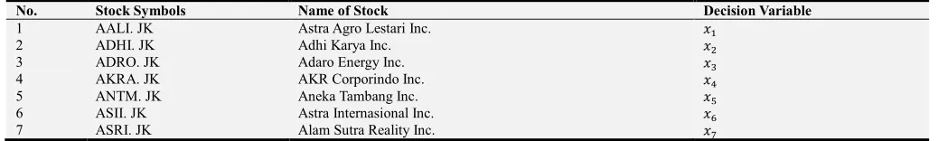
The first step in forming a model and decision making in the optimization of portfolio stock selection is to make a notation to represent the name of the stock to be examined, as shown in Table 1.
Table 1. Decision Variable for 16 Stock.
No. Stock Symbols Name of Stock Decision Variable
1 AALI. JK Astra Agro Lestari Inc.
2 ADHI. JK Adhi Karya Inc.
3 ADRO. JK Adaro Energy Inc.
4 AKRA. JK AKR Corporindo Inc.
5 ANTM. JK Aneka Tambang Inc.
6 ASII. JK Astra Internasional Inc.
No. Stock Symbols Name of Stock Decision Variable
8 BBCA. JK Bank Central Asia Inc.
9 BBNI. JK Bank Negara Indonesia Inc.
10 BBRI. JK Bank Rakyat Indonesia Inc.
11 BBTN. JK Bank Tabungan Indonesia Inc.
12 BMRI. JK Bank Mandiri Inc.
13 BSDE. JK Bumi Serpong Damai Inc.
14 BUMI. JK BUMI Resources Inc.
15 CPIN. JK Charoen Pokphand Indonesia Inc.
16 ELSA. JK Elnusa Inc.
b)Identifying Goal Constraints (Goal)
As for some of the objectives (investor) constraints that investors want to form a portfolio as follows:
Goal 1: Funds invested are only limited to Q.
Goal 2: Minimize the weight of the proportion of funds for each stock with the upper limit of Dm.
Goal 3: Maximize the expected return of realization of the portfolio with the lower limit of Em.
Goal 4: Minimize beta from a portfolio with an upper limit of Bm.
Goal 5: Minimize the standard deviation of the portfolio with the upper limit Sm.
c)Identifying Additional MGP Constraint
Starting from the assumption that investors are dissatisfied with the output produced with GP, the process of selecting portfolio stocks is continued by using a settlement method called MGP. The next section will discuss the selection of portfolio stocks with the Meta Goal Programming (MGP) model. Based on the knowledge of an investor added additional constraints as follows: Percentage of maximum deviation from all main objectives no more than the set limit (0.060), Percentage of maximum deviation from each main goal is not more than the set limit (0.71), and Minimum eight of nineteen fulfilled goals. In this study, the authors made a combination of each weight of three MGP types including: Combination A (ξ1,ξ2,ξ3) = (0,0,1), Combination B (ξ1,ξ2,ξ3)
=(0,1,0), dan Combination C (ξ1,ξ2,ξ3) = (1,0,0).
d)Formulation of the Portfolio Stock Selection Model
with Meta Goal Programming
Guided by various formulations that have been previously set, a general form of portfolio stock selection with the MGP model is obtained as follows.
1 1 2 2 3 3
min=ξ µ ξ µ ξ µ, , (9) Subject to
;
16 1Q
x
i i≤
∑
= (10)+ − = ; (11)
(
)
;
16 1 m s s i ii
x
n
p
E
R
E
+
−
=
∑
= (12);
16 1 m s s i ii
x
+
n
−
p
=
B
∑
=
β
(13);
19 19 16 1 m i ii
x
+
n
−
p
=
S
∑
=
σ
(14)∑
∈=
=
−
+
) 1 (;
...,
,
1
;
1 ) 1 ( ) 1 ( ) 1 ( k S i k k k i ii
Q
k
r
t
n
w
λ
µ
(15)2
0; 1,..., ;
i
i l
i
n
w D l r
t − ≤ = (16)
;
...,
,
1
;
2 ) 2 ( ) 2(
Q
l
r
D
l+
λ
l−
µ
l=
l=
(17);
,
...
,
1
;
;
0
i
S
(3)r
r
3y
M
d
M
i≤
i−
i i≤
∈
r=
−
(18);
...,
,
1
;
3 ) 3 ( ) 3 ( ) 3 ( ) 3 (r
r
Q
S
card
y
l r r r S ir
+
−
=
=
∑
∈
λ
µ
(19)
{ }
(3)3
0,1 , , 1,...,
i r
y ∈ i∈S r= r (20)
, 0, 1, 2,...,19 s s
n p ≥ s= (21)
≥ 0, (22)
(1) (1) (2) (2) (3) (3)
1 2 3
, , , , r , r , , , 0
k k l l
λ µ λ µ λ µ ξ ξ ξ ≥ (23)
The objective function equation that minimizes deviations from the additional purpose of 3 types of MGP with µ1 for
MGP type 1 deviation, µ2 MGP deviation type 2 and µ3 MGP
deviation type 3. Equation (5) the main constraint function which states the optimization of the limit of the number of funds invested Q. Constraints Equation (11) is an objective constraint which states that investors want the proportion of funds for each stock to be no more than the Dm limit.
Equation constraint (12) is an obstacle that states investors want to maximize return expectations with the lower limit of Em. Equation (13) states that investors want to minimize the
beta value of stocks with an upper limit of Bm. Equation (14)
expresses the willingness of investors to minimize the standard deviation of their portfolio and set the upper limit of
Sm. The constraint of equation (15) is a type 1 MGP
constraint which optimizes the percentage number of undesired deviation variables and not more or equal to Q1.
The constraints of equation (16) and equation (17) state that the maximum percentage deviation will not be more or equal to the limit of Q2. Equation constraints (18) and equation (19)
achieved that will not be more or equal to Q3. Equation
constraints (20) show binary variables with a value of 0.1 which means the goal is reached {yi = 0} and the goal is not
reached {yi = 1}. The constraint of equation (21) states that
ni, pi is greater or equal to zero which is a positive and negative deviation from the goal. Equation constraints (22) state the decision variable which is the set of real numbers. Equation constraints (23) state a decision variable that is greater or equal to zero. Based on the above model a
portfolio stock selection model has formed with the MGP method.
e)Application of the Portfolio Stock Selection with Meta Goal Programming Model
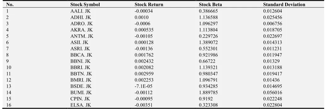
Before applying the stock selection model with LGP, it is necessary to look for the expected return, Beta, and Standard Deviation values of 16 stock samples whose values are listed in Tabel 2.
Table 2. Stock Return, Stock Beta, and Standard Deviation.
No. Stock Symbol Stock Return Stock Beta Standard Deviation
1 AALI. JK -0.00034 0.386665 0.012604
2 ADHI. JK 0.0010 1.136588 0.025456
3 ADRO. JK -0.0006 1.096297 0.006756
4 AKRA. JK 0.000535 1.113804 0.018705
5 ANTM. JK -0.00105 0.229726 0.022697
6 ASII. JK 0.000128 1.389072 0.014313
7 ASRI. JK -0.00136 0.552301 0.011231
8 BBCA. JK 0.001762 0.921986 0.011947
9 BBNI. JK 0.002432 0.66722 0.01329
10 BBRI. JK 0.002082 1.139321 0.013188
11 BBTN. JK 0.002959 0.980347 0.019417
12 BMRI. JK 0.002253 1.096791 0.01436
13 BSDE. JK -7.1E-05 0.934285 0.014695
14 BUMI. JK -0.00112 1.889785 0.056016
15 CPIN. JK -0.00095 0.9192 0.022248
16 ELSA. JK -0.00351 0.323308 0.022804
Furthermore, based on the data shown in Table 2 proportions or investment weights of each of the 16 stocks
are examined using the MGP model. The Portfolio Selection Model with MGP is as follows:
1 1 2 3 4
5 6 7 8
9 10 11 12
13 14
min
( /0.0625) + (
/0.0625) + ( /0.0625) + (
/0.0625)
+ ( /0.0625)+(
/0.0625) + (
/0.0625) + ( /0.0625)
( /0.0625) + (
/0.0625) +(
/0.0625) + (
/0.0625)
(
/0.0625) + (
/0.0625
p
p
p
p
p
p
p
p
p
p
p
p
p
p
ξ
=
+
+
15 1617 18 19
2
3 1 2 3 4 5 6
7 8 9 10 11 1
) + (
/0.0625) +(
/0.0625)
+ (
/0.0007) + (
/1.2369) + (
/0.0060))
( )
(( /19) + ( /19) + ( /19) + ( /19) + ( /19) + ( /19)
+ ( /19) ( /19) + ( /19) + (
/19) + (
/19) + (
p
p
n
p
p
D
y
y
y
y
y
y
y
y
y
y
y
y
ξ
ξ
+
+
+
213 14 15 16 17 18
19
/19)
+ (
/19) +(
/19) + (
/19) + (
/19) + (
/19) + (
/19)
+ (
/19))
y
y
y
y
y
y
y
Subject to: Hard Constraint:
16
1
1
xi
i
≤
∑
=
Good Constraint:
1 2 3
4 5 6
7 8 9
10 11 12
( 0.000343466 )+(0.00098215 )+( 0.000603158 )
+(0.000535347 )+( 0.001054838 ) +(0.000127793 )
+( 0.001361071 )+(0.001762194 )+(0.002431908 )
+(0.002081892
)+(0.002958968
)+(0.002252881
)
+(
x
x
x
x
x
x
x
x
x
x
x
x
− −
− −
13 14 15
16 17 17
0.0000708747
)+( 0.001115671
) + ( 0.000951334
)
+ ( 0.003509327
) +
= 0.0007
x
x
x
x
n
p
− − −
− −
1 2 3
4 5 6
7 8 9
10 11 12
(0.386664887 )+(1.136588167
)+(1.096297443 )
+(1.113803709
)+(0.229725682 ) +(1.389071981
)
+(0.552300873
+(0.921986123
+(0.667219559
)
+(1.139321486
) + (0.980346765
) + (1.096791423
)
+
x
x
x
x
x
x
x
x
x
x
x
x
13 14 15
16 18 18
(0.934285024
) + (1.889785047
) + (0.919200071
)
+ (0.323308474
) +
n
p
= 1.2369
x
x
x
x
−
1 2 3
4 5 6
7 8 9
10 11 12
(0.012603669 )+(0.025455703 )+(0.006756125 ) +(0.018704625 )+(0.02269734 ) +(0.014312663 ) +(0.011230785 )+(0.011946646 )+(0.013290345 ) +(0.013187807 ) + (0.019417071 ) + (0.014359896 )
+
x
x
x
x
x
x
x
x
x
x
x
x
13 14 15
16 19 19
(0.014695148 ) + (0.056016132 ) + (0.022248215 ) + (0.022804005 ) + n p = 0.0060
x
x
x
x
−s (0.0625 ) 0; = 1,2,...,16
p − D ≤ s
17 (0.0007 ) 0
n − D ≤
18 (1.2369 ) 0
n − D ≤
19 (0.0060 ) 0
n − D ≤
0.625 ps 0.625yj 0; s 1 2, ,...,16; j = , ,...,1 2 16
− ≤ − ≤ =
17 17
0.625 n 0.007y 0
− ≤ − ≤
18 18
0.625 p 12.369y 0
− ≤ − ≤
19 19
0.625 p 0.06y 0
− ≤ − ≤
1 2 3 4
5 6 7 8
9 10 11 12
13 14 15 16
/0.0625) + ( /0.0625) + ( /0.0625) + ( /0.0625)
+ ( /0.0625) + ( /0.0625) +( /0.0625)+( /0.0625)
+( /0.0625)+( /0.0625)+( /0.0625)+( /0.0625)
+( /0.0625)+( /0.0625)+( /0.0625)+(
(p p p p
p p p p
p p p p
p p p p
17 18 19 1 1
/0.0625)
+(n /0.0007)+(p /1.2369) + (p /0.0060) + λ −µ =0.060
2 2
+ 0 71
D λ −µ = .
16
1
3 3
+ = 8/19
19
j j
y
λ µ
= −
∑
{ }
0,1j
y ∈
, 0, 1, 2,...,19 s s
n p ≥ s=
≥ 0, = 1, … , 16
(1) (1) (2) (2) (3) (3)
1 2 3
, , , , r , r , , , 0
k k l l
λ µ λ µ λ µ ξ ξ ξ ≥
The results of portfolio stock optimization are obtained by using LINGO16 software. Optimization yields the optimal solution in the form of the selection of 5 stocks from 16 stocks that meet the predetermined criteria. The selected stocks will then be formed into an optimal portfolio.
4. Results and Discussion
The results of the selection of portfolio stocks with the MGP model obtained with LINGO 16 are presented in Table 3.
Table 3. Result of Optimization with Meta Goal Programming Model.
Stock Symbols Name of Stock Decision Variable Proportion
BBCA. JK Bank Central Asia Inc. 0.0625
BBNI. JK Bank Negara Indonesia Inc, 0.0625
BBRI. JK Bank Rakyat Indonesia Inc. 0.0625
BBTN. JK Bank Tabungan Indonesia Inc. 0.0625
Tabel 3 shows the results of the optimization in the form of five selected stocks and their respective weights. Variation A (ξ1,ξ2,ξ3) = (0,0,1) was chosen in this optimization, meaning
that the decision maker should prioritize the additional constraints of type 3 MGP in order to obtain an optimal portfolio. The following is presented in Table 4 a comparison of the calculation of returns, beta, and standard deviations for the stock market and new portfolios formed with the MGP model.
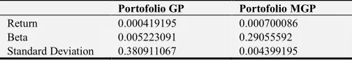
Table 4. Return, Beta, and Standard Deviation Portofolio with Meta Goal Programming.
Portofolio GP Portofolio MGP
Return 0.000419195 0.000700086
Beta 0.005223091 0.29055592
Standard Deviation 0.380911067 0.004399195
Based on (1), (2), and (3) the stock weights listed in Table 3 are used to obtain the return value, stock beta and portfolio standard deviation seen in Table 4. In Table 4 it can be seen that the return value obtained from the MGP model has a difference of 0.028 percent higher than GP portfolio return, the beta value obtained by MGP is also 29 percent higher than the beta value obtained by GP.
5. Conclusion
Based on the objectives set by investors, namely optimizing the proportion of investment funds up to 6.25 percent, maximizing the Return Portfolio, minimizing beta and standard deviation of the portfolio by utilizing the MGP model, five stocks will be formed into the optimal portfolio. These stocks include Bank Central Asia Inc., Bank Negara Indonesia Inc., Bank Rakyat Indonesia Inc., Savings Bank Indonesia Inc., And Bank Mandiri Inc.
Based on the results seen in Table 4 above, the selection of portfolio stocks using the MGP model managed to obtain a return value of 0.0007, this value is higher than the return value obtained from GP which is 0.000419195. The standard deviation obtained in the MGP portfolio of 0.29055592 is also lower than the GP standard deviation of 0.005223091. The difference in the beta value of GP stocks with MGP is 0.376511872. It can be concluded that the issue of stock selection with the MGP model produces a portfolio with a lower return value and standard deviation from the GP portfolio.
References
[1] H. Babaei, M. Tootooni, K. Shahanaghi and A. Bakhsha, Lexicographic goal programming approach for portofolio optimization, Journal of Industrial Engineering International, 9 (2009), 63-75.
[2] S. Bahloul and F. Abid, A combined analytic hierarchy process and goal programming approach to international portfolio selection in the presence of investment barriers, International Journal Multicriteria Decision Making, 3 (2013), 1-20. [3] L. J. Bain and M. Engelhardt, Introduction to Probability and
Mathematical Statistics, Duxbury, Pasific Grove, 1992. [4] A. K. Bhargava, S. R. Singh and D. Bansal, Production
planning using fuzzy meta goal programming model, Indian Journal of Science and Technology, 8 (2015), 34-42.
[5] J. P. Ignizio, Introduction to Linear Goal Programming, Sage Publication, California, 1985.
[6] D. Jones and M. Tamiz, A review of goal programming and its applications, Annals of Operations Research, 58 (1995), 39-53.
[7] D. Jones and M. Tamiz, Practical goal programming, Springer, London, 2010.
[8] F. Kucukbay and C. Araz, A comparison of fuzzy goal programming and linear physical programming, An International Journal of Optimization and Control, 6 (2016), 121-128.
[9] K. D. Lawrence, D. R. Pai and S. M. Lawrence, A multi criteria meta goal programming model based in morningstar sector grouping, Applications of Management Science, 17 (2015), 19-25.
[10] H. W. Lin, S. V. Nagalingam and G. C. I. Lin, Manufacturing decision-support using interactive meta goal programming, Australian Research, 2007, 331-341.
[11] H. Markowitz, Portofolio selection, The Journal of Finance, 7 (1952), 77-91.
[12] A. M. Parra, A. B. Terol and M. V. R. Uria, A fuzzy goal programming approach to portofolio selection, European Journal of Operational Research, 133 (2001), 287-297. [13] H. Sakhari and M. Sabuohi, Application meta goal
programming in agriculture case study Neyshabour city, Journal of Agricultural Economics and Development, 26 (2012), 17.
[14] M. V. R. Uria, R. Caballero, F. Ruiz, and C. Romero, Meta goal programming, European Journal of Operational Research, 2002, 422-429.
[15] M. R. T. Yazdi, S. Fallahpour, dan M. A. Moghaddam, Portfolio Selection using Meta Goal Programming and Extended Lexicographic Goal Programming, ResearchGate Journal of Financial Research, 2017, 591-612.