1 2 3 4 5 6 7 8 9 10 11 12 13 14 15 16 17 18 19 20 21 22 23 24 25 26 27 28 29 30 31 32 33 34 35 36 37 38 39 40 41 42 43 44 45 46 47 48 49 50 51 52 53 54 55 56 57 58
Electricity consumption probability density forecasting method based on
LASSO-Quantile Regression Neural Network
Yaoyao Hea,b,∗, Yang Qina,b, Shuo Wangc, Xu Wangd, Chao Wangd aSchool of Management, Hefei University of Technology,Hefei 230009, China
bKey Laboratory of Process Optimization and Intelligent Decision-Making (Hefei University of Technology), Ministry of Education, Hefei 230009, China
cSchool of Computing and Digital Technology Birmingham City University Millennium Point, Curzon Street, Birmingham, B4 7XG, England, UK
d China Institute of Water Resources and Hydropower Research, Beijing 100048, China
Abstract
The electricity consumption forecasting is a challenging task, because the predictive accuracy is easily
affected by multiple external factors, such as society, economics, environment, as well as the renewable
en-ergy, including hydro power, wind power and solar power. Particularly, in the smart grid with large amount
of data, how to extract valuable information of those external factors timely is the key to the success of
electricity consumption forecasting. A method of probability density forecasting based on Least Absolute
Shrinkage and Selection Operator-Quantile Regression Neural Network (LASSO-QRNN) is proposed in this
paper. First, important features are extracted from external factors affecting the electricity consumption
forecasting by LASSO regression. Then, the LASSO-QRNN model is constructed to predict annual
elec-tricity consumption. The results of elecelec-tricity consumption forecasting under different quantiles in the next
several years are evaluated. Besides, we introduce kernel density estimation into our LASSO-QRNN model,
which can give a probability distribution instead of a single-valued prediction. The prediction accuracy is
evaluated through the empirical analyses from the Guangdong province dataset in China and the California
dataset in the United States. The simulation results demonstrate that the proposed method provides better
performance for electricity consumption forecasting, in comparison with existing quantile regression neural
network (QRNN), back-propagation of errors neural network (BP), radial basis function neural network
(RBF) methods, quantile regression (QR) and nonlinear quantile regression (NLQR). LASSO-QRNN can
not only better learn the high-dimensional data in electricity consumption forecasting, but also provide more
precise results.
Keywords: LASSO Quantile Regression Neural Network, probability density forecasting, electricity
consumption forecasting, uncertainty analysis, high dimensional data
2 3 4 5 6 7 8 9 10 11 12 13 14 15 16 17 18 19 20 21 22 23 24 25 26 27 28 29 30 31 32 33 34 35 36 37 38 39 40 41 42 43 44 45 46 47 48 49 50 51 52 53 54 55 56 57 58 59
1. Introduction
Electricity consumption around the world is rising rapidly, due to the ever-increasing population, value
pursuit for better living standards and attention to large-scale industrialization, which leads to the positive
economic growth rates [1]. Medium and long term electricity consumption forecasting is essential to energy
investment planning [2]. For example, in response to the excessive consumption of electricity, huge quantities
of fossil fuel were used to generate electricity at the end of the 20th century, which caused the depletion of
fossil fuel resources. Since the beginning of the 21st century, renewable energy sources (such as hydro, solar,
wind) have been increasingly utilized to generate electricity. Compared with traditional fossil fuels, the wind,
solar and hydro power generations have the advantages of large development potential, non-pollution and
recyclability. They established a better and cleaner energy structure. However, on account of the uncertainty
and complementarity of hydro, wind and solar power, electricity consumption forecasting becomes utterly
important, but challenging. An accurate forecasting can promote the effective use of renewable energy.
Moreover, precise electricity consumption forecasting can guide government strategies for future energy
usage and development.
Most commonly used methods for electricity consumption forecasting include regression models [3], time
series models [4], the fuzzy theory [5], neural networks [6], Bayesian networks [7], hybrid method [8] and so
on. Regression analysis and time series models are the most acclaimed modeling techniques in electricity
consumption forecasting [9]. With the rapid development of modern artificial intelligence methods, artificial
neural network and population evolutionary algorithm are introduced into electricity forecasting [10].
Gra-diti G et al. [11] demonstrated that statistical machine learning approaches provided more accurate power
predictions. In terms of prediction output, existing methods of electricity consumption forecasting can be
divided into deterministic point prediction and probabilistic forecasting based on uncertainty analysis [12].
An exact point prediction cannot reflect the fluctuation of electricity consumption. In reality, real electricity
consumption and the load growth are influenced by various factors, including economic development,
in-dustrial structure, income level of residents, climate, geographical environment, national policy (electricity
price) etc. All of these factors interact and influence each other. Furthermore, the integration of
informati-zation and industrialiinformati-zation in power industry promotes the rapid growth of power data, resulting in a large
number of data with extensive sources, diverse features, huge volume and fast growth. It makes electricity
consumption forecasting increasingly complicated [13].
To deal with the uncertainty in electricity consumption, a new Kullback-Liebler (K-L) divergence based
similarity measure strategy was designed by Shao et al. [14] to forecast the electricity demand in China
considering the significant impact factors of the electricity consumption, showing better accuracy. Amina
∗Corresponding author. School of Management, Hefei University of Technology,Hefei 230009, China
Email addresses: [email protected](Yaoyao Hea,b,∗),[email protected](Yang Qina,b),[email protected] (Shuo Wangc),[email protected](Xu Wangd),[email protected](Chao Wangd)
2 3 4 5 6 7 8 9 10 11 12 13 14 15 16 17 18 19 20 21 22 23 24 25 26 27 28 29 30 31 32 33 34 35 36 37 38 39 40 41 42 43 44 45 46 47 48 49 50 51 52 53 54 55 56 57 58
et al. [15] implemented a novel fuzzy wavelet neural network model for electricity consumption forecasting
in the power system of the Greek Island of Crete, which provided significantly better results. In [16], a
small-sample adaptive hybrid model (AHM) based on trend extrapolation method was proposed to forecast
electricity consumption in China from 1991 to 2014, which showed robustness to stochastic changes and
obtained more precise forecasting results. Al-Ghandoor et al. [17] presented an empirical model based on
multivariate linear regression of time series for the Jordanian industrial sector, which identified the main
influential factors of electricity consumption. Van der Meer et.al reviewed the probabilistic forecasting of
photovoltaic power production and electricity consumption [18] and proposed a probabilistic forecasting
method using Gaussian processes [19]. Vincenzo Bianco et al. [20] developed a long-term forecasting model
considering the influence of economic and demographic variables on the annual electricity consumption in
Italy from 1970 to 2007. It utilized the linear regression to build different models to reduce the uncertainty
of forecasting, and showed consistency with the official projections.
As a kind of probabilistic forecasting method [21], probability density forecasting method not only can
get the future electricity consumption variation interval under the corresponding confidence interval, but
also depict the full probability distributions of the future electricity consumption. It can provide more
insights into the distribution of electricity consumption, which can help power system decision-makers to
make effective decisions for the power system to avoid the large error and economic losses. However, owing to
the complexity and uncertainty of external influence factors, existing probability density forecasting methods
are difficult to characterize the uncertainty of electricity consumption [22].
In order to achieve accurate prediction of electricity consumption in large data environments, extracting
the feature from the external factors has become a key problem. The dimension of explanatory variables will
increase remarkably, if all influential factors are considered without selection. Identifying the most related
factors for training the model can improve predictive performance and reduce computational cost [23].
Traditional variable selection methods, such as forward stepwise, backward stepwise, ridge regression, may
suffer from the co-linearity problem, if there are too many tedious independent variables in high-dimensional
situations. So, it is likely to lose some important factors in the process of feature selection, greatly reducing
the explanatory power of the model. To tackle this issue, Tibshirani [24] proposed the Least Absolute
Shrinkage and Selection Operator (LASSO) algorithm, which was further extended by Hastie, Tibshirani
and Friedman [25]. By constructing a penalty function to acquire a refined model, the algorithm can compress
the coefficients of variables and make some regression coefficients set exactly to zero, so as to achieve the aim
of variable selection [26]. The LASSO is computationally practicable for high-dimensional data, reducing
amounts of computation greatly. For example, Florian et al. [27] proposed an accurate method of wind power
forecasting combined with LASSO, greatly reducing the computation time under the condition of the vast
parameter space. Huebner et al. [28] utilized LASSO regression for variable selection from different types
2 3 4 5 6 7 8 9 10 11 12 13 14 15 16 17 18 19 20 21 22 23 24 25 26 27 28 29 30 31 32 33 34 35 36 37 38 39 40 41 42 43 44 45 46 47 48 49 50 51 52 53 54 55 56 57 58 59
recognize the patients at high risk of disease progression using the LASSO method from the high-dimensional
microarray data. In the paper, we first present a novel method, namely LASSO-quantile regression neural
network (LASSO-QRNN), to combine the LASSO regression with the quantile regression neural network
(QRNN).
QRNN model was put forward by Taylor [30], which is a nonparametric nonlinear method combing the
neural network with the quantile regression. Dadabada et al. [31] used the particle swarm algorithm to
opti-mize the QRNN for predicting the volatility of financial time series. Cannon [32] applied the QRNN method
to the precipitation downscaling task, considering the characteristics of prediction with mixed
discrete-continuous variables. Xu et al. [33] proposed a composite quantile regression neural network (CQRNN)
model to solve underlying nonlinear problems among variables. He et al. [34] utilized the quantile regression
neural network method to implement the probability density forecasting of wind power, which validly
quan-tified the indeterminacy of wind power generation. These empirical studies show the superiority of QRNN
method. Not only can it reveal the entire conditional distribution of response variables, but also deal with
complex nonlinear problems. In this paper, we will make use of the superior performance of QRNN for
electricity consumption forecasting. It can produce the detailed conditional quantiles of the consumption
values, and more accurate predictions.
Motivated by the existing research, we propose a new learning method to predict electricity consumption,
which combines LASSO and QRNN. The details will be given in the next section. LASSO can produce
high-quality features and reduce data dimensions effectively. QRNN is used to build the model, which estimates
the probability density function of the consumption value. To the best our knowledge, this is the first work
that uses and combines LASSO and QRNN for electricity consumption prediction. We verify our method on
two real-world datasets from Guangdong province in China and California in U.S. The probability density
forecasting results from the LASSO-QRNN method are compared to the results without considering the
external factors and the results without variable selection considering the external factors. Comparisons
with the state of the art further exhibit that the LASSO-QRNN method is able to improve the forecasting
accuracy of the electricity consumption significantly and minimize the uncertainty in electricity consumption.
The main contributions of this article include: 1) LASSO dimension reduction technique is applied
to reduce the uncertainty of annual electricity consumption associated with social and economic factors.
2) At different quantiles, LASSO-QRNN produces the probability distribution of electricity consumption
in details. More smooth probability density curves can be obtained, which provides more insights into
electricity consumption. 3) Two criteria are utilized to evaluate the performance of LASSO-QRNN, namely,
mean absolute percentage errors (MAPE) and relative mean squared error (RMSE). 4) The superiority of
the method is proven through the experiment on two real-world data sets, Guangdong province in China
and California in U.S. We study and compare three different settings: without considering external factors,
considering external factors without variable selection and considering external factors with LASSO-QRNN
2 3 4 5 6 7 8 9 10 11 12 13 14 15 16 17 18 19 20 21 22 23 24 25 26 27 28 29 30 31 32 33 34 35 36 37 38 39 40 41 42 43 44 45 46 47 48 49 50 51 52 53 54 55 56 57 58
method. Our results indicate that the proposed LASSO-QRNN method provides informative prediction
than QRNN. Meanwhile, it achieves better accuracy than radial basis function neural network (RBF) [35],
back-propagation of errors neural network (BP) [36], quantile regression (QR) [37] and nonlinear quantile
regression (NLQR) [38]. In conclusion, the main novelty of the proposed method consists in effectively
reducing data dimensions and nondeterminacy in the forecasting process to improve prediction precision
considering the external and internal factors.
The subsequent sections are organized as follows. Section 2 introduces the correlation theories including
the mechanism of LASSO regression and the mathematical formulation of QRNN. Section 3 proposes the
LASSO-QRNN method for electricity consumption. The simulation studies are conducted to evaluate the
performance of LASSO-QRNN in Section 4. Finally, conclusions are given in Section 5.
2. Correlation theory
2.1. LASSO regression
With the advent of the big data era, how to extract useful information from data has been paid close
attention by scholar. One of the most effective approaches is statistical modeling technology. In order to
reduce model deviation at the beginning of modeling, researchers usually consider adding as many
indepen-dent variables as possible. However, in the actual modeling process, the subset of indepenindepen-dent variables are
chosen in order to improve the prediction accuracy. It is called the variable selection. Variable selection is
an all-important step in the process of statistical modeling [39].
The LASSO method is a contraction estimation method, which can effectively deal with complex
high-dimensional data problems [40].
A multivariate linear regression model that satisfies the classical hypothesis is shown below.
Y =Xβ+ε (1)
whereεi ∼i.i.dN(0, σ2)means that each residual term is independent and has the same distribution with normal distribution. The response variables satisfy the condition Y ∼ N(Xβ, σ2I) , in which I is the
identity matrix. By optimizing the objective function Eq(2), the ordinary least squares estimation result
obtained isβˆols= (X′X)−1X′Y .
min
β
1
2∥Y −Xβ∥
2
2 (2)
Suppose the row and the column from the design matrix are respectively recorded as sand k. If s < k,
2 3 4 5 6 7 8 9 10 11 12 13 14 15 16 17 18 19 20 21 22 23 24 25 26 27 28 29 30 31 32 33 34 35 36 37 38 39 40 41 42 43 44 45 46 47 48 49 50 51 52 53 54 55 56 57 58 59
Tibshirani [24] added L1 penalty to the end of the Eq(2) as follows.
min
β
1
2∥Y −Xβ∥
2 2+
λ
2 ∥β∥1 (3)
whereλis penalty parameter that is positive correlated with punishment intensity,∥β∥1is 1-norm satisfying
∥β∥1=|β1|+|β2|+· · ·+|βk|. In the formula, the first item is the loss function, which measures the fitting effect of the regression model on the data. And the second item is the penalty function, which condenses
some nonsignificant coefficients into 0. By optimizing the Eq(3), the regression coefficient vector estimation
ˆ
βlasso can be obtained, which is called LASSO regression. There is an equivalent constraint form that corresponds to the Eq(3) as follows.
min
β
1
2∥Y −Xβ∥
2 2
s.t. ∥β∥1≤C
(4)
where C is the constraint parameter corresponding to λ, which is negative correlation with punishment
intensity. The optimal solution can be obtained by Eq(3) and Eq(4). Because the penalty function is a
first order function with absolute value, it cannot be solved by the calculus method. It requires highly
complicated numerical calculation to solve the regression equation. Efron et al. [41] proposed least angle
regression (LARS) algorithm to solve the planning problem. By using LARS algorithm to solve LASSO
regression efficiently, LASSO algorithm is highly regarded by the academic community.
2.2. Quantile regression Neural network (QRNN)
Koenker and Bassett presented a method of quantile regression (QR). Compared with the traditional
mean regression, QR can more accurately describe the influence of the conditional distribution shape and the
variation range of the dependent variables for independent variables. However, this method only learns the
linear relationship between the response variables and the input variables under different quantiles, which
is not appropriate for the nonlinear relationship in most practical data [42]. Therefore, Taylor put forward
a nonlinear QR method based on neural networks. The expression is shown as follows.
Qyi(τ|xi) =f(xi, Ti(τ), Ui(τ)), i= 1,2, ..., n (5)
f(xi, Ti(τ), Ui(τ)) =g2{ K
∑
k=1
ui,k(τ)g1[
J
∑
j=1
ti,j,k(τ)xi]} (6)
where τ ∈ (0,1) is able to generate different quantiles, Ti = {ti,j,k}j=1,2,···,J;k=1,2,···,K represents the estimated weight matrix between the input layer and the hidden layer,Ui={ui,k}k=1,2,···,K represents the connection weight vector between the hidden layer and the output layer. g1(·)is expressed as an activation
2 3 4 5 6 7 8 9 10 11 12 13 14 15 16 17 18 19 20 21 22 23 24 25 26 27 28 29 30 31 32 33 34 35 36 37 38 39 40 41 42 43 44 45 46 47 48 49 50 51 52 53 54 55 56 57 58
function of the hidden layer using the hyperbolic tangent sigmoid functiong1(v) =1+1e−v.g2(·)is the output
layer function, which is represented by a general linear model. f(xi, Ti(τ), Ui(τ)) is a nonlinear function that is composition of weight vectorsTiand Ui.
The parameter estimation values ofT(τ) ={T1, T2,···, Tn}, U(τ) ={U1, U2,···, Un}in the QRNN model can be acquired by a programming problem as follows.
H(T(τ), U(τ)) = min
n
∑
i=1
ρτ[(yi(τ)−f(xi, Ti(τ), Ui(τ))] +s1
∑
i,j,k
t2i,j,k+s2
∑
i,k
u2i,k (7)
where nis the number of the sample, ρτ is loss function defined as following Eq(8). s1 and s2 are model penalty parameters, which effectively prevent the model from overfitting to improve the accuracy of
predic-tion. The optimal estimate value ofT(τ)andU(τ)can be obtained by optimizing Eq(7), which are recorded
as Tˆ(τ) and Uˆ(τ). With bringing the two values into Eq(5), the conditional quantiles of the response
variables are obtained.
ρτ(u) =
τ u
(τ−1)u
, u≥0
, u <0
(8)
3. Electricity consumption probability density forecasting method based on LASSO-QRNN
3.1. LASSO-QRNN model
It is known that electricity consumption forecasting is disturbed by diverse external factors and these
factors influence the accuracy of forecasting greatly. How to identify significant factors that influence the
electricity consumption becomes important. Based on LASSO-QRNN method, the paper mainly explores
the influence of historical load and external factors on the electricity consumption forecasting.
The estimate value of the parameters can be obtained by solving the programming problem in Eq(7).
However, when the influence factors in the model are voluminous considering the influence of historical load
and external factors on electricity consumption forecasting, the variable selection method ought to be used
to improve the prediction accuracy. The LASSO regression method is used in this paper, which is based on
the original objective function of QRNN and adds theL1 penalty. The model is shown as follows.
min
n
∑
i=1
ρτ[(yi(τ)−f(xi, Ti(τ), Ui(τ))] +s1
∑
i,j,k
t2i,j,k+s2∑
i,k
u2i,k+λ(∥T(τ)∥1+∥U(τ)∥1) (9)
whereλ is penalty parameter that is positive correlation with punishment intensity,∥T(τ)∥1 and ∥U(τ)∥1
are 1-norm. In the formula, the first item is the loss function, which measures the fitting effect of the QRNN
model on the data. The second item is the penalty function, which can compress nonsignificant coefficients
into zero. Then, the process of variable selection is achieved. In order to solve the LASSO-QRNN model,
2 3 4 5 6 7 8 9 10 11 12 13 14 15 16 17 18 19 20 21 22 23 24 25 26 27 28 29 30 31 32 33 34 35 36 37 38 39 40 41 42 43 44 45 46 47 48 49 50 51 52 53 54 55 56 57 58 59
min
n
∑
i=1
ρτ[(yi(τ)−f(xi, Ti(τ), Ui(τ))] +s1 ∑
i,j,k
t2i,j,k+s2 ∑
i,k
u2i,k
s.t. ∥T(τ)∥1+∥U(τ)∥1≤C
(10)
in whichC is the constraint parameter corresponding toλ. The smaller the value ofC is, the stronger the
effect of compressing the coefficients into zero is. Furthermore, the programming problem can be solved
by using LARS algorithm proposed by Efron, so as to obtain the parameter estimates of the model and
the conditional quantile of the electricity consumption. The LASSO-QRNN model not only produces the
distribution of electricity consumption values in different quantiles, but also selects more explanatory factors
to reduce the data dimension. In conclusion, the LASSO-QRNN method optimizes the prediction model,
which lays the foundation for the follow-up prediction work.
3.2. Probability density forecasting method based on LASSO-QRNN with kernel density estimation
Kernel density estimation (KDE) method is a nonparametric method for estimating probability density
functions [43], fitting observations to simulate a true probability distribution by a smooth spike function.
According to the above research, the conditional quantile of electricity consumption in different quantiles
can be obtained, which is represented as Zi =Qyi(τ|xi). The conditional quantile Zi is utilized as the input values of the kernel function. In addition, by choosing appropriate bandwidth for probability density
prediction, the probability density functions of electricity consumption are obtained eventually. Supposing
that Z1, Z2, . . . , Zn are the independent identically distributed random samples, the probability density function at any one point is denoted asf. The formula is shown as follows.
ˆ
fh(x) =
1
n
n
∑
i=1
Kh(x−Zi) =
1
nh
n
∑
i=1
K(x−Zi
h ) (11)
wherehis the bandwidth that is a smoothing parameter requiring self-actuated setting,nis the sample size,
andK(·)is regarded as a non-negative kernel function. Among different kernel functions, such as gaussian, rectangular, triangular, epanechnikov, biweight, cosine and optcosine, this paper chooses epanechnikov and
gaussian, because the predicted results are more precise compared with the other kernel functions through
contrast experiments. The function expressions are respectively shown as follows.
K(u) =3 4(1−u
2)
s.t. |u| ≤1
(12)
K(u) = √1 2πe
−1 2u
2
(13)
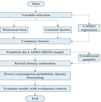
The flow chart of electricity consumption probability density forecasting method based on LASSO-QRNN
in this paper is shown in Fig.1.
2 3 4 5 6 7 8 9 10 11 12 13 14 15 16 17 18 19 20 21 22 23 24 25 26 27 28 29 30 31 32 33 34 35 36 37 38 39 40 41 42 43 44 45 46 47 48 49 50 51 52 53 54 55 56 57 58
Start
Historical load
Compress factors
Establish the LASSO-QRNN model
Kernel density estimation
Power consumption probability density forecasting
Evaluate results with evaluation criteria
Conditional quantile
End
Variable selection
LASSO regression External factors
2 3 4 5 6 7 8 9 10 11 12 13 14 15 16 17 18 19 20 21 22 23 24 25 26 27 28 29 30 31 32 33 34 35 36 37 38 39 40 41 42 43 44 45 46 47 48 49 50 51 52 53 54 55 56 57 58 59
4. Experimental Analysis
4.1. Evaluation criteria
In this section, we compare LASSO-QRNN with two other situations to show the benefit of introducing
LASSO in our method. 1) the QRNN without considering external factors; 2) the QRNN considering
external factors without variable selection. Then, LASSO-QRNN is also compared with other
state-of-the-art approaches in electricity consumption forecasting, including RBF, BP, QR and NLQR. To verify the
effectiveness of our method, the paper employs the following evaluation criteria:
The mean absolute percentage errors (MAPE) is used for error analysis to point prediction results.
MAPE is defined as follows.
M AP E= 1
n
n
∑
i=1 yi−yˆi
yi
(14)
in which n indicates the total number of years for electricity consumption to be predicted, yi and yˆi respectively represent the actual and predicted values of electricity consumption at time i.
The relative mean square errors (RMSE) is used to reflect the deviation degree of the predicted value to
the actual value. RMSE is defined as follows.
RM SE=
n
∑
i=1
(yi−yˆi)2
n
∑
i=1 yi2
(15)
4.2. Case study 1: Guangdong province in China
The first case is from Guangdong province of China. The experimental data are available from Guangdong
Statistical Yearbook published in 2017 [44]. As a dominating electricity consumption province in China,
the electricity consumption in Guangdong province can reach the sum of the surrounding provinces and
cities [45]. In terms of electricity consumption structure and energy efficiency, the proportion of coal in
fuel sources has declined, and the proportion of high-quality energy (including hydro, solar, wind, etc) in
consumption has increased. In recent years, accompanied by the economic development and the adjustment
of industrial structure, the electricity consumption in Guangdong province has achieved sustainable growth,
which is shown in Fig. 2. Hence, it is important to predict electricity consumption accurately.
In this case study, the historical electricity consumption and external factors from the past four years
are used as input data to forecast the annual electricity consumption. Suppose Yt= (yt−1, yt−2, . . . , yt−c) indicates the historical load of the lag c, in which c represents the maximum lag phase of the electricity
consumption sequence ytto be predicted. The sequence of external influence factors is expressed as Xt=
(X1
2 3 4 5 6 7 8 9 10 11 12 13 14 15 16 17 18 19 20 21 22 23 24 25 26 27 28 29 30 31 32 33 34 35 36 37 38 39 40 41 42 43 44 45 46 47 48 49 50 51 52 53 54 55 56 57 58
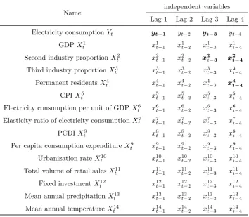
Table 1: The statement of independent variables for Guangdong province data
Name independent variables Lag 1 Lag 2 Lag 3 Lag 4
Electricity consumptionYt yt−1 yt−2 yt−3 yt−4
GDP X1
t x1t−1 x1t−2 x1t−3 x1t−4
Second industry proportionX2
t x2t−1 x2t−2 x2t−3 x2t−4
Third industry proportion X3
t x3t−1 x3t−2 x3t−3 x3t−4
Permanent residentsX4
t x4t−1 x4t−2 x4t−3 x4t−4
CPIX5
t x5t−1 x5t−2 x5t−3 x5t−4
Electricity consumption per unit of GDPXt6 x6t−1 x6t−2 x6t−3 x6t−4
Elasticity ratio of electricity consumptionXt7 x7t−1 x7t−2 x7t−3 x7t−4
PCDIXt8 x8t−1 x8t−2 x8t−3 x8t−4
Per capita consumption expenditure X9
t x9t−1 x9t−2 x9t−3 x9t−4
Urbanization rateX10
t x10t−1 x10t−2 x10t−3 x10t−4
Total volume of retail salesX11
t x11t−1 x11t−2 x11t−3 x11t−4
Fixed investmentX12
t x12t−1 x12t−2 x12t−3 x12t−4
Mean annual precipitationX13
t x13t−1 x13t−2 x13t−3 x13t−4
Mean annual temperatureX14
t x14t−1 x14t−2 x14t−3 x14t−4
factor Xd
t satisfies the conditionXtd= (xdt−1, xdt−2, . . . , xdt−q). In the case, mis set to 14. In addition, both
cand qare equal to 4. There are 60independent variables in total, as shown in Table.1. LASSO regression
is used to select the most influential factors of electricity consumption. The selected factors are historical
load with a lag of 1 and 3 periods, second industry proportion with a lag of 3 and 4 periods and permanent
residents with a lag of 4 periods, as shown in boldface text of Table.1. The procedure chart of compressing
factors is shown in Fig. 3. The dotted line indicates the trajectory of the factor selection process. The
abscissa indicates the constraint coefficientC, and the ordinate indicates the regression coefficientβ. The
two coefficients correspond to the parameters in Eq(4). From the output of LASSO, we can see that the
electricity consumption in Guangdong province closely correlates with the historical electricity consumption,
the secondary industry proportion and the permanent residents. The description of the pertinent literature
further reflects this result [46]. During 1995-2016, with the development of the city, the number of permanent
residents in Guangdong province is growing and the second industry has achieved great development, which
leads to the growth of electricity consumption.
The annual total electricity consumption and extracted factors from 1995 to 2016 are selected as
2 3 4 5 6 7 8 9 10 11 12 13 14 15 16 17 18 19 20 21 22 23 24 25 26 27 28 29 30 31 32 33 34 35 36 37 38 39 40 41 42 43 44 45 46 47 48 49 50 51 52 53 54 55 56 57 58 59
1995 2000 2005 2010 2015
100
200
300
400
500
Time/year
Electr
icity consumption/T
wh
Figure 2: The electricity consumption in Guangdong Province from 1995 to 2016
*
*
* *
*
*
**
***
*
*
**
*****
*
**
*
*
*
**
0.0
0.2
0.4
0.6
0.8
1.0
0.000
0.010
0.020
St
and
ard
iz
ed C
oeffici
ents
*
*
* *
*
*
*
*
**
*
*
***************
*
*
*
* *
*
* **
***
*
****************
*
*
* *
*
*
**
*****
***************
*
*
* *
*
* **
***
*
***
*****
*
**
*
*
*
**
*
*
* *
*
* **
**
*
*
*
**
*****
*
**
*
*
*
**
*
*
* *
*
* **
**
*
*
*
**
*****
*
**
*
*
*
**
*
*
* *
*
* **
**
*
*
*
**
*****
*
**
*
*
*
**
*
*
* *
*
*
**
**
*
*
***********
*
*
*
**
*
*
* *
*
* **
***
*
***
*****
*
**
*
*
*
**
*
*
* *
*
* **
***
*
***
*****
*
**
*
*
*
**
*
*
* *
*
* **
***
*
***
*****
*
**
*
*
*
*
*
*
*
* *
*
* **
***
*
***
*****
*
**
*
*
*
**
*
*
* *
*
* **
***
*
***
*****
*
**
*
*
*
**
*
*
* *
*
* **
***
*
*
******
*
*
*
*
*
*
*
**
*
*
* *
*
* **
***
*
***
*****
*
**
*
*
*
*
*
*
*
* *
*
* **
***
*
**
*
*****
*
**
*
*
*
**
LASSO
32
15
17
0
1
2
4
13
Figure 3: The procedure chart of compressing factors (Guangdong)
2 3 4 5 6 7 8 9 10 11 12 13 14 15 16 17 18 19 20 21 22 23 24 25 26 27 28 29 30 31 32 33 34 35 36 37 38 39 40 41 42 43 44 45 46 47 48 49 50 51 52 53 54 55 56 57 58
factors from 1995 to 2010. Through rolling forecasting method, the historical electricity consumption and
influence factors in previous four years are considered as input variables to forecast the annual electricity
consumption. The electricity consumption values for a total of 12 years from 1999 to 2010 are the expected
output values. In other words, a total of 12 groups of samples are selected to train the LASSO-QRNN
model, then we can further determine the optimal structure of the neural network. According to the
opti-mal structure, the electricity consumption values from 2011 to 2016 are predicted. Without considering the
external factors, the input layer of the neural network structure is 4 nodes, the hidden layer is 1 node, and
the output layer is 1 node. Considering external influence factors without variable selection, the nodes of
input layer, hidden layer and output layer are 60, 1, 1, respectively. When the LASSO regression is used for
variable selection considering external influence factors, the input structure of the neural network structure
is 5 nodes, the hidden layer is 1 node, and the output layer is 1 node. The neural network training number
is set to 100. And the penalty parameter is set to 2, which denotes thats1 ands2 are equal to 2 in Eq(7).
Through the trained neural network structure, consecutive quantiles under different quantiles from 2011 to
2016 are obtained, which have been restored from normalization. This paper selects the quantile range from
0.01 to 0.99, and the interval is 0.05. Then the predicted electricity consumption quantile is used as the
input variable of epanechnikov kernel function. Combined with the kernel density estimation method, the
annual probability density curve from 2011 to 2016 is obtained.
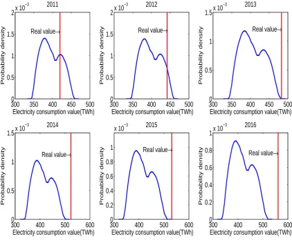
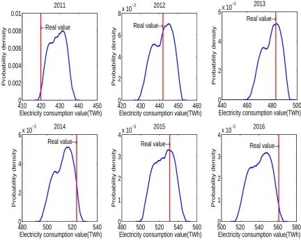
Fig. 4 shows the probability density curve from 2011 to 2016 without considering the external factors. We
compare it with the one with factor selection, as shown in Fig. 5. In Figs. 4 and 5, the value of the abscissa
corresponding to the red vertical line represents the actual value of the annual electricity consumption in
Guangdong province of China. The following conclusions can be drawn: Without considering the external
factors, the true values almost deviate from the highest probability point of the probability density curve.
Most of the true values appear at the end of the probability density curve, and the predicted values are far
from the true values. However, in consideration of external factors with variable selection, the true values
are almost in the vicinity of the highest probability point in the probability density curve. There is almost
no case in the tail of the probability density curve. The probability density forecasting method based on
LASSO-QRNN can produce better probability density curve of predicted values closer to the true values.
To show the effect of variable selection in our method, we compare three situations as we introduced
earlier: QRNN without considering external factors, QRNN considering external factors without variable
selection and LASSO-QRNN considering external factors, as shown in the Table. 2. According to the Table. 2,
the MRPE and RMSE of the predicted values considering the external factors are smaller than those without
considering the external factors in the mode and median. Moreover, considering the external factors, the
MRPE and RMSE of the predicted values with variable selection are smaller than those without variable
selection in the mode and median. It can be concluded that the predicted results using the LASSO-QRNN
2 3 4 5 6 7 8 9 10 11 12 13 14 15 16 17 18 19 20 21 22 23 24 25 26 27 28 29 30 31 32 33 34 35 36 37 38 39 40 41 42 43 44 45 46 47 48 49 50 51 52 53 54 55 56 57 58 59
3000 350 400 450 500 0.5
1 1.5
2x 10
−3 2011
Electricity consumption value(TWh)
Probability density
Real value→
3000 350 400 450 500 0.5
1 1.5
2x 10
−3 2012
Electricity consumption value(TWh)
Probability density
Real value→
3000 350 400 450 500 0.5
1 1.5x 10
−3 2013
Electricity consumption value(TWh)
Probability density
Real value→
3000 400 500 600 0.5
1 1.5x 10
−3 2014
Electricity consumption value(TWh)
Probability density
Real value→
3000 400 500 600 0.2
0.4 0.6 0.8 1
x 10−3 2015
Electricity consumption value(TWh)
Probability density
Real value→
3000 400 500 600 0.2
0.4 0.6 0.8
1x 10
−3 2016
Electricity consumption value(TWh)
Probability density
Real value→
Figure 4: Probability density curve without considering the external factors in Guangdong province of
China
2 3 4 5 6 7 8 9 10 11 12 13 14 15 16 17 18 19 20 21 22 23 24 25 26 27 28 29 30 31 32 33 34 35 36 37 38 39 40 41 42 43 44 45 46 47 48 49 50 51 52 53 54 55 56 57 58
4100 420 430 440 450 0.002
0.004 0.006 0.008 0.01
2011
Electricity consumption value(TWh)
Probability density
←Real value
4200 430 440 450 460 2
4 6 8x 10
−3 2012
Electricity consumption value(TWh)
Probability density
Real value→
4400 460 480 500 2
4 6x 10
−3 2013
Electricity consumption value(TWh)
Probability density
Real value→
4800 500 520 540 2
4 6x 10
−3 2014
Electricity consumption value(TWh)
Probability density
Real value→
4800 500 520 540 560 1
2 3 4x 10
−3 2015
Electricity consumption value(TWh)
Probability density
Real value→
5000 520 540 560 580 1
2 3 4x 10
−3 2016
Electricity consumption value(TWh)
Probability density
Real value→
Figure 5: Probability density curve considering the external factors (LASSO) in Guangdong province of
2 3 4 5 6 7 8 9 10 11 12 13 14 15 16 17 18 19 20 21 22 23 24 25 26 27 28 29 30 31 32 33 34 35 36 37 38 39 40 41 42 43 44 45 46 47 48 49 50 51 52 53 54 55 56 57 58 59
Table 2: Prediction errors in three situations of Guangdong province data
Evaluation criteria Without considering external factors (QRNN)
Considering external factors
QRNN LASSO-QRNN
MRPE(%) Median 15.41 8.60 1.83
Mode 21.21 5.25 1.21
RMSE(%) Median 3.22 1.10 0.05
Mode 5.63 0.50 0.02
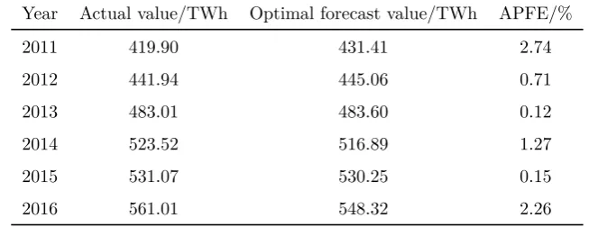
Table 3: Forecasting results of Guangdong province data based on LASSO-QRNN
Year Actual value/TWh Optimal forecast value/TWh APFE/%
2011 419.90 431.41 2.74
2012 441.94 445.06 0.71
2013 483.01 483.60 0.12
2014 523.52 516.89 1.27
2015 531.07 530.25 0.15
2016 561.01 548.32 2.26
considering the external factors. The predicted results of the mode is slightly better than the median and
the MRPE are 1.21 % and 1.83 %, respectively. In the big data environment with smart grid, this shows
that probability density forecasting of electricity consumption ought to fully consider the external influential
factors to achieve the purpose of optimal prediction model from the perspective of high dimensional data
analysis.
Based on the probability density forecasting method of LASSO-QRNN, we present the optimal point
predictions and absolute percentage forecast errors (APFE) of annual electricity consumption from 2011
to 2016, as shown in Table. 3. In consideration of external factors, the MAPE of the probability density
forecasting based on LASSO-QRNN is 1.21%. The minimum APFE of the probability density prediction
is 0.12 %. It can be concluded from Table. 3 that the probability density forecasting method based on
LASSO-QRNN can obtain more accurate prediction results, which are close to the actual value.
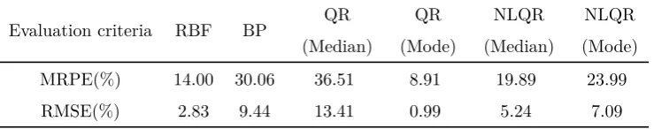
More details on the state of the art are provided to better illustrate the advantages of LASSO-QRNN
method. The paper compares the prediction error obtained from LASSO-QRNN with the error obtained by
RBF [35], BP [36], QR [37] and NLQR [38] in Table. 4. LASSO-QRNN method shows significantly better
performance, reducing the indeterminacy of electricity consumption forecasting.
2 3 4 5 6 7 8 9 10 11 12 13 14 15 16 17 18 19 20 21 22 23 24 25 26 27 28 29 30 31 32 33 34 35 36 37 38 39 40 41 42 43 44 45 46 47 48 49 50 51 52 53 54 55 56 57 58
Table 4: Prediction errors of state-of-the-art methods for Guangdong province data
Evaluation criteria RBF BP QR (Median)
QR
(Mode)
NLQR
(Median)
NLQR
(Mode)
MRPE(%) 14.00 30.06 36.51 8.91 19.89 23.99
RMSE(%) 2.83 9.44 13.41 0.99 5.24 7.09
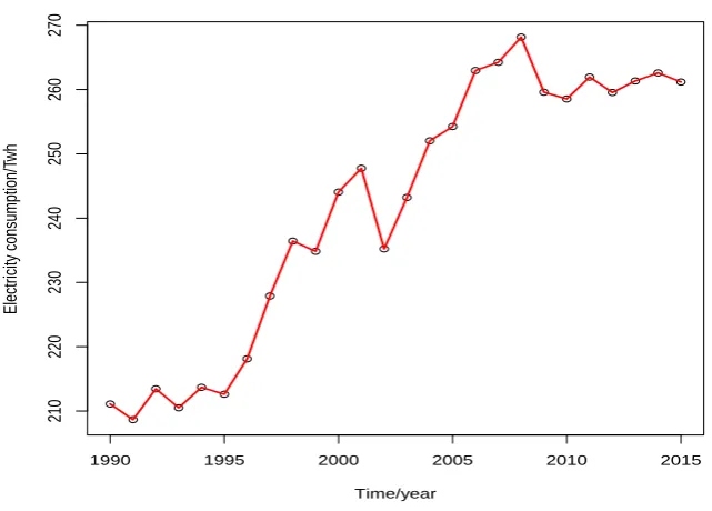
4.3. Case study 2: California in U.S.
The second case is from California in U.S. The experimental data are available from U.S. Energy
Infor-mation Administration website [47], which contains annual historical retail sales (consumption) of electricity
and external factors including total energy, average electricity price, number of electricity consumers and
so on. California’s electricity generation, transmission and distribution network are a management system
with a wide range and complexity [48]. Its fuel sources include higher percentages of natural gas, hydro, and
non-hydro renewables, and lower percentages of coal, petroleum, and nuclear [49]. Until 2003, the level of
electricity consumption in California ranked the second among the 50 states. The electricity consumption
in California from 1990 to 2015 is presented in Fig. 6. It shows a declining period after the peak value of
electricity consumption in 2008, which increases the difficulty and challenge tremendously for forecasting
the electricity consumption. In [50], the statewide annual electricity consumption prediction was
pre-sented during the period 2008-2018, assuming average temperatures. It is worth noting that the electricity
consumption in California used in this paper is different from that in this literature.
According to the above observations, the uniform rolling forecast approach is employed to forecast the
annual electricity consumption in California, and the number of external factorsmis set to 8. In addition,
both c and q are equal to 4. As can be seen in Table.4, there are 36 independent variables in total.
In this case, the LASSO regression is also adopted to select the most appropriate variables for electricity
consumption forecasting. The procedure chart of compressing factors is shown in Fig. 7. The selected factors
are total energy with a lag of 1 ,2 and 4 periods, average electricity price with a lag of 1 and 4 periods,
and number of electricity customers with a lag of 2 and 3 periods, as shown in bold section of Table. 5. As
similar as [51], it appears that economic growth and the fluctuation of electricity price are the main factors
correlated with electricity consumption. Similarly to the previous case study, LASSO regression alleviates
high-dimensional data problems through the selection process of key factors, which is of great significance
in reality.
The electricity consumption and influence factors from 1990 to 2009 are used as the training sample.
Similar to the Guangdong province case, the rolling forecasting method is also adopted to process data. The
electricity consumption values for a total of 16 years from 1994 to 2009 are the expected output values. As
2 3 4 5 6 7 8 9 10 11 12 13 14 15 16 17 18 19 20 21 22 23 24 25 26 27 28 29 30 31 32 33 34 35 36 37 38 39 40 41 42 43 44 45 46 47 48 49 50 51 52 53 54 55 56 57 58 59
Table 5: The statement of independent variables for California data
Name independent variables Lag 1 Lag 2 Lag 3 Lag 4
Electricity consumptionYt yt−1 yt−2 yt−3 yt−4
Personal incomeX1
t x1t−1 x1t−2 x1t−3 x1t−4
Population X2
t x2t−1 x2t−2 x2t−3 x2t−4
Per capita personal income X3
t x3t−1 x3t−2 x3t−3 x3t−4
Personal consumption expendituresX4
t x4t−1 x4t−2 x4t−3 x4t−4
GDP X5
t x5t−1 x5t−2 x5t−3 x5t−4
Total energyXt6 x6t−1 x6t−2 x6t−3 x6t−4
Average electricity priceXt7 x7t−1 x
7
t−2 x7t−3 x7t−4
Number of electricity customersXt8 x8t−1 x8t−2 x 8
t−3 x
8
t−4
1990 1995 2000 2005 2010 2015
210
220
230
240
250
260
270
Time/year
Electr
icity consumption/T
wh
Figure 6: The electricity consumption of California from 1990 to 2015
2 3 4 5 6 7 8 9 10 11 12 13 14 15 16 17 18 19 20 21 22 23 24 25 26 27 28 29 30 31 32 33 34 35 36 37 38 39 40 41 42 43 44 45 46 47 48 49 50 51 52 53 54 55 56 57 58
****
**
*
*
*
*
*
***
* ******
*****
* *
*
*
**
**
*
**
*
*
*
***
*
*
*
*
*
* *
0.0
0.2
0.4
0.6
0.8
1.0
−
0.01
0.0
1
0.03
Standardiz
ed Coefficients
****
**
*
*
*
*
*
***
*
****
*******
* *
*
*
**
**
***********
*
*
*
* *
****
**
*
*
*
*
*
***
* ******
***
**
* *
*
*
**
**
***
*
*
*
***
*
*
*
*
*
* *
****
**
*
*
*
*
*
***
* ******
***
**
* *
*
*
**
*
*
*
*
*
*
*
*
***
*
*
*
*
*
*
*
****
**
*
*
*
*
*
***
* ******
***
**
* *
*
*
*
*
**
*
**
*
*
*
***
*
*
*
*
*
*
*
****
**
*
*
*
*
*
***
* ******
***
**
* *
*
*
**
**
***
*
*
*
***
*
*
*
*
*
* *
****
**
*
*
*
*
*
***
* ******
***
**
* *
*
*
**
**
*
**
*
*
*
***
*
*
*
*
*
* *
****
**
*
*
*
*
*
***
* ******
***
**
* *
*
*
**
**
*
**
*
*
*
***
*
*
*
*
*
* *
****
**
*
*
*
*
*
***
* ******
***
**
*
*
*
*
**
*
*
*
*
*
*
*
*
***
*
*
*
*
*
* *
*
*
**
*
*
*
*
*
*
*
***
* *
**
***
***
*
*
*
*
*
*
*
*
**
*
**
*
*
*
**
*
*
*
*
*
*
*
*
****
**
*
*
*
*
*
**
*
* *********
**
* *
*
*
**
**
***
*
*
*
***
*
*
*
*
*
* *
****
**
*
*
*
*
*
***
* ***********
* *
*
*
**
**
***
*
*
*
***
*
*
*
*
*
* *
****
**
*
*
*
*
*
***
* *
*****
***
**
* *
*
*
**
**
*
**
*
*
*
***
*
*
*
*
*
* *
**
**
**
*
*
*
*
*
***
* ***********
* **
*
**
**
***
*
*
*
***
*
*
*
*
*
* *
****
**
*
*
*
*
*
**** ***********
* *
*
*
**
**
***
*
*
*
***
*
*
*
*
*
* *
****
**
*
*
*
*
*
***
* ******
*****
* *
*
*
**
**
***
*
*
*
***
*
*
*
*
*
* *
****
**
*
*
*
*
*
***
* ******
***
**
* *
*
*
**
**
***
*
*
*
***
*
*
*
*
*
* *
****
**
*
*
*
*
*
***
* ******
***
**
* *
*
*
**
**
***
*
*
*
***
*
*
*
*
*
* *
****
**
*
*
*
*
*
***
* ***********
* *
*
*
**
**
***
*
*
*
***
*
*
*
*
*
* *
****
*
*
*
*
*
*
*
***
* ******
***
**
* *
*
*
**
**
***
*
*
*
***
*
*
*
*
*
* *
****
**
*
*
*
*
*
***
* ******
***
**
* *
*
*
**
**
***
*
*
*
***
*
*
*
*
*
* *
LASSO
13
4
17
24
0
8
17
26
31
45
Figure 7: The procedure chart of compressing factors (California)
neural network for obtaining the optimal structure. From 2010 to 2015, a total of six years of electricity
consumption forecasting is implemented. Without considering the external factors, the input layer of the
neural network is 4 nodes. Considering external influence factors without variable selection, the node number
of input layer is 36. When LASSO regression is used for variable selection considering external influence
factors, the input structure of the neural network is 7 nodes. In all three settings, the hidden layer is 2
nodes, and the output layer is 1 node. The neural network training number is set to 10, and the penalty
parameter is set to 5. Then the predicted electricity consumption quantile is considered as the input variable
of Gaussian kernel function, which have been inversely normalized. Through the trained neural network
structure and kernel density estimate algorithm, the results of probability density forecasting under different
quantiles for any year from 2010 to 2015 are obtained.
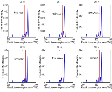
From the above, the probability density curve of consecutive quantiles can be obtained from 2010 to 2015.
Fig. 8 shows the probability density curve from 2010 to 2015 without considering the external factors. Similar
to the previous case study, it is compare with the results considering external factors with variable selection,
as shown in Fig. 9. In Figs. 8 and 9, the value of the abscissa corresponding to the red vertical line indicates
the actual value of the annual electricity consumption in California, USA.We obtain the following findings:
Without considering the external factors, the true values almost deviate from the highest probability point of
2 3 4 5 6 7 8 9 10 11 12 13 14 15 16 17 18 19 20 21 22 23 24 25 26 27 28 29 30 31 32 33 34 35 36 37 38 39 40 41 42 43 44 45 46 47 48 49 50 51 52 53 54 55 56 57 58 59
Nevertheless, the true values are almost all in the vicinity of the highest probability point in the probability
density curve considering the external factors. Therefore it is easy to find that the LASSO-QRNN method
can acquire consecutive and slippy the probability density curves. It means that the predicted values are
more likely to get close to the true values. The probability density curve can not only provide more detailed
information for electricity consumption forecasting, but also open up new ideas and methods for electricity
consumption forecasting.
200
0
250
300
0.005
0.01
0.015
0.02
0.025
2010
Electricity consumption value(TWh)
Probability density
Real value
→
200
0
250
300
0.005
0.01
0.015
0.02
0.025
2011
Electricity consumption value(TWh)
Probability density
Real value
→
200
0
250
300
0.01
0.02
0.03
2012
Electricity consumption value(TWh)
Probability density
Real value
→
200
0
250
300
0.01
0.02
0.03
0.04
2013
Electricity consumption value(TWh)
Probability density
Real value
→
200
0
250
300
0.01
0.02
0.03
0.04
2014
Electricity consumption value(TWh)
Probability density
Real value
→
200
0
250
300
0.01
0.02
0.03
0.04
2015
Electricity consumption value(TWh)
Probability density
Real value
→
Figure 8: Probability density curve without considering the external factors in California of U.S
In order to illustrate the effectiveness of this method, as similar as the case above-mentioned, the
pre-diction error of the three situations are also compared in Table. 6. According to the experimental results
in Table. 6, the MRPE and RMSE of the predicted results considering the external factors are less than
the predicted results without considering the external factors in the median. It can be concluded that the
predicted results using the LASSO-QRNN method for variable selection are better than the predicted results
2 3 4 5 6 7 8 9 10 11 12 13 14 15 16 17 18 19 20 21 22 23 24 25 26 27 28 29 30 31 32 33 34 35 36 37 38 39 40 41 42 43 44 45 46 47 48 49 50 51 52 53 54 55 56 57 58
220
0
240
260
280
300
2
4
6
8
x 10
−3
2010
Electricity consumption value(TWh)
Probability density
Real value
→
220
0
240
260
280
300
2
4
6
8
x 10
−3
2011
Electricity consumption value(TWh)
Probability density
Real value
→
220
0
240
260
280
2
4
6
8
x 10
−3
2012
Electricity consumption value(TWh)
Probability density
Real value
→
220
0
240
260
280
2
4
6
8
x 10
−3
2013
Electricity consumption value(TWh)
Probability density
Real value
→
220
0
240
260
280
2
4
6
8
x 10
−3
2014
Electricity consumption value(TWh)
Probability density
Real value
→
220
0
240
260
280
2
4
6
8
x 10
−3
2015
Electricity consumption value(TWh)
Probability density
Real value
→
2 3 4 5 6 7 8 9 10 11 12 13 14 15 16 17 18 19 20 21 22 23 24 25 26 27 28 29 30 31 32 33 34 35 36 37 38 39 40 41 42 43 44 45 46 47 48 49 50 51 52 53 54 55 56 57 58 59
Table 6: Prediction errors in three situations of California data
Evaluation criteria Without considering external factors (QRNN)
Considering external factors
QRNN LASSO-QRNN
MRPE(%) Median 7.44 2.09 1.29
Mode 3.12 3.89 2.04
RMSE(%) Median 0.56 0.05 0.02
Mode 0.10 0.16 0.05
Table 7: Forecasting results of California data based on LASSO-QRNN
Year Actual value/TWh Optimal forecast value/TWh APFE/%
2010 258.33 259.76 0.48
2011 261.94 258.45 1.33
2012 259.54 257.31 0.86
2013 261.33 256.72 1.77
2014 262.59 257.07 2.10
2015 261.17 258.07 1.19
without variable selection and without considering the external factors. The predicted results of the median
is slightly better than the mode and the MRPE are 1.29% and 2.04%, respectively. This demonstrates
that the electricity consumption probability density forecasting method based on LASSO-QRNN is able to
lessen the nondeterminacy caused by external factors for improving the prediction precision of electricity
consumption, thus avoiding larger prediction errors and economic losses.
The forecasting results considering external factors based on LASSO-QRNN are shown in Table. 7, which
includes actual values, optimal point forecasts and the APFE of electricity consumption in California during
the period of 2010-2015. From Table. 7, it can be seen that the MAPE of the probability density forecasting
based on LASSO-QRNN is 1.29%. In addition, the minimum APFE of the probability density prediction
is 0.48%. Consequently, it can be concluded that the probability density forecasting method based on
LASSO-QRNN can obtain high-precision prediction results.
Similar to the case of Guangdong province data, the prediction error obtained by LASSO-QRNN is also
compared with that of BP, RBF, QR and NLQR as shown in Table. 8. The prediction accuracy of BP, RBF,
QR and NLQR is lower than that of LASSO-QRNN for California data, which justifies the superiority of
the proposed method.
2 3 4 5 6 7 8 9 10 11 12 13 14 15 16 17 18 19 20 21 22 23 24 25 26 27 28 29 30 31 32 33 34 35 36 37 38 39 40 41 42 43 44 45 46 47 48 49 50 51 52 53 54 55 56 57 58
Table 8: Prediction errors of state-of-the-art methods for California data
Evaluation criteria RBF BP QR (Median)
QR
(Mode)
NLQR
(Median)
NLQR
(Mode)
MRPE(%) 6.28 7.05 7.06 3.87 2.02 2.08
RMSE(%) 0.40 0.50 0.50 0.16 0.04 0.05
5. Conclusions
Aiming at the electricity consumption forecasting, this paper proposes a probability density forecasting
method – LASSO-QRNN. Firstly, the method selects the most informative features from external factors by
using LASSO. It reduces data dimensions effectively without hurting predictive performance Secondly, the
QRNN method produces overall probability distribution of the electricity consumption at different quantiles
in details, which is valuable information for managing electricity consumption. The performance of
LASSO-QRNN is analyzed on two real-world datasets from Guangdong province of China and California of U.S.
Our main findings are:
By taking into account the external factors, the MRPE and RMSE of the probability density forecasting
results using LASSO-QRNN method are smaller than those without considering the external factors in terms
of the median and mode. With respect to the probability density prediction curve, the true values are almost
all in the vicinity of the highest probability point in the probability density curve considering the external
factors. However, the probability of the true value appearing in the tail is significantly increased if the
external factors are not considered. Derived from the probability density curve, the MRPE considering the
external factors is limited within 2% by using LASSO-QRNN method. Furthermore, the comparative
analy-sis with QRNN, RBF, BP, QR and NLQR displays that our method provides a more accurate prediction and
reduces the uncertainty of electricity consumption forecasting in power systems. From the simulation results,
the most relevant factors affecting electricity consumption in different regions are significantly discrepant.
The historical electricity consumption, second industry proportion and permanent residents are selected as
the feature to train the model in the data of Guangdong province, while total energy, average electricity
price and number of electricity customers are selected to train the model for the U.S. data. The sequence
diagram of Guangdong province data (Fig.2) is monotonically increasing other than the California data,
which verifies that the electricity consumption of California (Fig.6) is more intractable to achieve accurate
prediction than Guangdong data for the aggravation of instability. In summary, LASSO-QRNN is capable
of important features and learning from high-dimensional data effectively. It produces more informative
2 3 4 5 6 7 8 9 10 11 12 13 14 15 16 17 18 19 20 21 22 23 24 25 26 27 28 29 30 31 32 33 34 35 36 37 38 39 40 41 42 43 44 45 46 47 48 49 50 51 52 53 54 55 56 57 58 59
ACKNOWLEDGEMENT
This paper is funded by the National Natural Science Foundation (No.71771073,71401049,U1765201),
the CRSRI Open Research Program (Program SN CKWV2017525/KY) and the Open Research Fund of
State Key Laboratory of simulation and Regulation of Water Cycle in River Basin (China Institute of Water
Resources and Hydropower Research) (Grant NO IWHR-SKL-201605).
References
[1] Pao HT. Forecasting energy consumption in taiwan using hybrid nonlinear models. Energy 2009;34(10):1438–144611. [2] Kaytez F, Taplamacioglu MC, Cam E, Hardalac F. Forecasting electricity consumption: A comparison of regression
analysis, neural networks and least squares support vector machines. International Journal of Electrical Power & Energy Systems 2015;67(67):431–8.
[3] Ming M, Niu D. Annual electricity consumption analysis and forecasting of china based on few observations methods. Energy Conversion & Management 2011;52(2):953–7.
[4] Sadownik R, Barbosa EP. Short-term forecasting of industrial electricity consumption in brazil. Journal of Forecasting 1999;18(3):215–24.
[5] Torrini FC, Souza RC, Oliveira FLC, Pessanha JFM. Long term electricity consumption forecast in brazil: A fuzzy logic approach. Socio-Economic Planning Sciences 2016;54:18–27.
[6] Azadeh A, Ghaderi SF, Sohrabkhani S. Annual electricity consumption forecasting by neural network in high energy consuming industrial sectors. Energy Conversion & Management 2008;49(8):2272–8.
[7] Bassamzadeh N, Ghanem R. Multiscale stochastic prediction of electricity demand in smart grids using bayesian networks. Applied energy 2017;193:369–80.
[8] Fan S, Chen L. Short-term load forecasting based on an adaptive hybrid method. IEEE Transactions on Power Systems 2006;21(1):392–401.
[9] Abdel-Aal RE, Al-Garni AZ. Forecasting monthly electric energy consumption in eastern saudi arabia using univariate time-series analysis. Energy 1997;22(22):1059–69.
[10] Taylor JW. Triple seasonal methods for short-term electricity demand forecasting. European Journal of Operational Research 2010;204(1):139–52.
[11] Graditi G, Ferlito S, Adinolfi G. Comparison of photovoltaic plant power production prediction methods using a large measured dataset. Renew