Primate Biol., 4, 143–151, 2017 https://doi.org/10.5194/pb-4-143-2017
© Author(s) 2017. This work is distributed under the Creative Commons Attribution 3.0 License.
ar
ticle
Estimation of baboon daily travel distances by means of
point sampling – the magnitude of underestimation
Holger Sennhenn-Reulen1,2, Langhalima Diedhiou3, Matthias Klapproth1, and Dietmar Zinner1
1Cognitive Ethology Laboratory, German Primate Center, Leibniz-Institute for Primate Research,
Kellnerweg 4, 37077 Göttingen, Germany
2Leibniz ScienceCampus “Primate Cognition”, German Primate Center/Leibniz Institute for Primate Research,
Kellnerweg 4, 37077 Göttingen, Germany
3Direction Parc National du Niokolo-Koba, Tambacounda, Senegal
Correspondence to:Dietmar Zinner (dzinner@gwdg.de)
Received: 28 March 2017 – Revised: 29 May 2017 – Accepted: 2 June 2017 – Published: 10 July 2017
Abstract. Daily travel distance (DTD), the distance an animal moves over the course of the day, is an important metric in movement ecology. It provides data with which to test hypotheses related to energetics and behaviour, e.g. impact of group size or food distribution on DTDs. The automated tracking of movements by applying GPS technology has become widely available and easy to implement. However, due to battery duration constraints, it is necessary to select a tracking-time resolution, which inevitably introduces an underestimation of the true underlying path distance. Here we give a quantification of this inherent systematic underestimation of DTDs for a terrestrial primate, the Guinea baboon. We show that sampling protocols with interval lengths from 1 to 120 min underestimate DTDs on average by 7 to 35 %. For longer time intervals (i.e. 60, 90, 120 min), the relative increase of deviation from the “true” trajectory is less pronounced than for shorter intervals. Our study provides first hints on the magnitude of error, which can be applied as a corrective when estimating absolute DTDs in calculations on travelling costs in terrestrial primates.
1 Introduction
Spatial information is crucial for many questions in ecologi-cal and behavioural research, e.g. species or resource distri-bution, habitat utilisation and estimates of home ranges or daily travel paths. The application of a satellite-supported global positioning system (GPS) has improved the collec-tion and accuracy of spatial data (Kays et al., 2015), provid-ing ecologists and behavioural biologists with opportunities to determine spatial patterns and test spatially explicit hy-potheses. Similarly, the use of GPS has become more preva-lent in primate field studies (Osborne and Glew, 2011; Ster-ling et al., 2013). Beside the determination of geograph-ical positions of ecologgeograph-ical objects or structures within a primate’s home range – such as sleeping and resting sites, feeding patches or seed-dispersal events – spatial data have been used to estimate home ranges (position, shape and size), habitat utilisation, and daily travel paths and travel
dis-tances. In primatology, the application of GPS collars indi-cated great potential particularly for semi-terrestrial primates in (semi-)open habitats (Markham and Altmann, 2008), but also for arboreal species (Stark et al., 2017).
Either animals can be equipped with a GPS device, and the respective positions will be collected automatically at pre-programmed intervals, or a researcher follows an animal and determines the positions using a handheld device (e.g. see Table 1). The GPS device consumes energy for every loca-tion fix, and thus battery life limits the number of posiloca-tion attempts or fixes a device can do. Programming fewer GPS fixes results in longer battery life but at the price of lower data density. It might not be a big problem if one is inter-ested in the area an animal uses within a year, which one
can probably estimate fairly well with just 2 or 3 fixes day−1
Table 1.A selection of GPS fixing intervals applied in primate and non-primate studies.
Species Sampling interval Device Reference
Papio anubis “Continuously” at 1 Hz Collar Strandburg-Peshkin et al. (2015) Chlorocebus 15 min Collar Isbell and Bidner (2016) Papio ursinus 20 min Collar Hoffman and O’Riain (2012) Papio ursinus 1 h Collar Pebsworth et al. (2012a, b) Papio cynocephalus 1 h Collar Markham and Altmann (2008) Macaca fuscata 1 h Collar Sprague et al. (2004)
Nasalis concolor 1 h Collar Stark et al. (2017)
Papio ursinus 3 h Collar Hoffman and O’Riain (2012) Rhinopithecus bieti 2–5 fixes day−1 Collar Ren et al. (2008)
Rhinopithecus bieti 2–5 fixes day−1 Collar Ren et al. (2009) Gorilla beringei 30 s Handheld Wright et al. (2015) Papio cynocephalus 5 min Handheld Johnson et al. (2015) Papio ursinus Average 9 min Handheld Bonnell et al. (2015) Chiropotes sagulatus Average 10 min Handheld Gregory et al. (2014) Papio ursinus 20 min Handheld Hoffman and O’Riain (2012) Macaca silenus 30 min Handheld Santhosh et al. (2015) Rhinopithecus bieti 30 min Handheld Grueter et al. (2008) Hoolock leuconedys 30 min Handheld Sarma and Kumar (2016)
Equus caballus 5 s for 6.5 days Collar Hampson et al. (2010) Panthera tigris 1–3 h Collar Naha et al. (2016) Capra hircus 2 h Collar Chynoweth et al. (2015) Elephas maximus 8 h Collar Alfred et al. (2012) Canis lupus 0.25, 1.5, 2, 6, 12 h Collar Mills et al. (2006)
e.g. 1 fix s−1 (1 Hz). In many studies, a trade-off between
long battery life for collecting data over a longer time pe-riod to estimate annual home ranges and a high data density to estimate DTD is sought. In particular the number of fixes per day used to estimate DTDs can influence the accuracy of the estimates and can make comparative studies within and between species difficult (e.g. Johnson et al., 2015).
Uncertainties in animal movement data, owing e.g. to sam-pling frequency, may strongly influence interpretations of tracking data (Bradshaw et al., 2007; Harris and Blackwell, 2013; Laube and Purves, 2011). As expected, in a number of studies it was shown that, as sampling intervals increase, the uncertainty of the behaviour between fixes increases; e.g. DTDs estimated from low sampling frequencies were signif-icantly shorter than those based on higher sampling frequen-cies (Laundré et al., 1987; Mills et al., 2006; Reynolds and Laundré, 1990; Rowcliffe et al., 2012; Edelhoff et al., 2016). How, if at all, this effect can be corrected statistically or by modelling is an open question (Blackwell et al., 2016; Flem-ing et al., 2014a, b, 2016; Shamoun-Baranes et al., 2011). One way to mitigate these effects can be an empirical es-timation of the magnitude of error one yields by applying different sampling frequencies.
In a study on range use of Guinea baboons (Papio
pa-pio) in the Niokolo-Koba National Park (Parc National du
Niokolo-Koba, PNNK), Senegal, we equipped baboons with Tellus ultra-light GPS remote ultra-high-frequency (UHF)
collars (Televilt, TVP Positioning AB, Lindesberg, Sweden; nowadays Followit AB). Since the main purpose of the ap-plication of GPS collars was to estimate home ranges of the baboons rather than an analysis of DTDs and since battery longevity was limited, we programmed the collars to take
only 10 fix day−1(seven fixes between 06:00 and 18:00 at 2 h
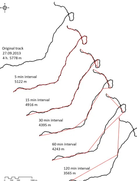
intervals, and three fixes at night at 21:00, 00:00 and 03:00) but over a longer period (on average 10 months). Even with a sampling interval of 2 h and thus just seven location points per day (the night-time fixes were not used since the baboons remained mainly stationary during the night), it was possible to approximate DTDs which could at least be used for inter-individual comparisons within the same population, given that the error in estimating DTDs was similar for all collared baboons. However, absolute DTDs were expected to be much longer than those approximations based on just seven loca-tion points (Fig. 1), making estimaloca-tions on actual travelling costs unreliable and comparisons of DTDs with other studies problematic.
Figure 1.Example of a baboon track line (black) over 4 h and esti-mated travel distances if sampling is done applying different inter-val lengths (respective red lines).
GPS device recording a continuous track. Further, one can expect that if a baboon moves more or less in a straight line the error might be smaller than in cases when the ba-boons meander a lot (e.g. Postlethwaite and Dennis, 2013). We therefore explored which particular travel behaviours of the baboons resulted in a greater or smaller deviation from the true DTD.
2 Methods
2.1 Study site and subjects
The study was carried out in the Niokolo-Koba National Park at the research station of the German Primate Center in
Si-menti (13◦0103400N, 13◦1704100W). The habitat consists of a
forest–savannah mosaic with seasonally flooded grassland, dry deciduous forest and gallery forest along the Gambia River. The climate is characterised by a dry season from November until May and a rainy season from June until Oc-tober.
The baboon community in Simenti comprises 350–400 in-dividuals. They live in a multi-level society consisting of one-male units (OMUs), parties and gangs (Patzelt et al., 2014;
Goffe et al., 2016). The baboons were habituated to human observers, so that observations and follows could be done from less than 5 m distance.
We selected four males from different parties, and one of us (Langhalima Diedhiou) followed on foot one individual baboon at a time, keeping a distance of 5 m to the respec-tive focal animal. The follows were repeated several times for each male (Table 2). The respective tracks were recorded with a handheld Garmin GPSMAP 62. Tracing set-up was “auto-normal”. In sum we recorded 56 2 h tracks. In nine cases we experienced gaps in the continuous recording of
the respective tracks (leg time>60 s). We deleted these nine
tracks from our analyses.
2.2 Statistical analysis
2.2.1 Deviation from true travel distance
Using a GPS device, even a continuous track consists of a number of fixes, optimally with a very short sampling inter-val or leg time. Leg time is the delta between the time stamps of the two fixes bounding the leg (e.g. 1 s if the sampling fre-quency is 1 Hz). However, since conditions are not always optimal, the real leg time varies and is most often larger than the targeted 1 s leg time. As a result, when we overlaid the continuous track with a 1 min sampling interval, for instance, the respective 1 min time stamps did not necessarily match with a fix from the GPS device. For instance, the closest time stamps can be at 57 or 62 s instead of 60 s. Therefore we had to interpolate the tracks and re-discretise them.
We artificially re-discretised the original tracks with reg-ular sampling intervals of 1, 2, 5, 10, 15, 30, 60, 90 and
120 min (shown on the x axis of Figs. 3 and 4) by using
linear interpolation between coordinates from the original tracks where necessary. This was achieved using the func-tion “redisltraj” in the “adehabitatLT” R package (Calenge, 2006). The deviation from the original travel distance is the difference between the original travel distance and the travel distance of the re-discretised version.
To get to a relationship between the deviation from the original travel distance and the re-discretisation sampling in-terval duration, we fitted a Bayesian multilevel log-normal regression model using the Stan-based (Stan Development Team, 2015) R add-on package brms (Bürkner, 2017), with
track index as grouping factorγi. The conditional mean of
the deviation from the original travel distanceyacross the
re-discretisation sampling interval duration range oft∈ [1,120]
was modelled as a −y15 transformed response (log-normally
distributed, therefore with a loge link function) on the
ba-sis of the linear predictorβ0+β1·t+β2·loge(t)+γi, which
Table 2.Temporal distribution of tracking periods. Tracking periods were either 4 or 2 h long. ID: individual baboon males; numbers in first horizontal line indicate hours of the day. T: tracking periods included in analysis; t: tracking periods excluded, because of gaps in the continuous tracking larger than 60 s.
ID Date (dd.mm.yyyy) 5 6 7 8 9 10 11 12 13 14 15 16 17 18
MST 08.09.2013 T T T T T T
MST 09.09.2013 T T t t T T
SNE 10.09.2013 T T
JKY 14.09.2013 T T T T
OSM 15.09.2013 T T
MST 16.09.2013 T T
SNE 18.09.2013 T T T T
JKY 19.09.2013 t t
MST 20.09.2013 t t T T T T
SNE 21.09.2013 t t T T
OSM 23.09.2013 T T T T
OSM 25.09.2013 T T T T
JKY 26.09.2013 t t T T
SNE 27.09.2013 T T t t
JKY 28.09.2013 T T T T
OSM 06.10.2013 t t T T
JKY 07.10.2013 T T T T
JKY 19.10.2013 T T T T
MST 20.10.2013 T T T T
OSM 21.10.2013 T T T T
SNE 22.10.2013 T T T T
JKY 23.10.2013 T T T T T T
OSM 24.10.2013 T T T T T T
MST 25.10.2013 t t T T T T
SNE 26.10.2013 t t T T T T
JKY 27.10.2013 T T T T T T
more details on the applied statistical approach, as well as
posterior mean and credible interval estimates forβ0β1β2.
2.2.2 Hidden Markov model
To be able to further quantify how the deviation from the original travel distance is related to moving velocity and turning-angle states, we fitted a hidden Markov model (Michelot et al., 2016). As an example, we performed this for a re-discretisation duration of 5 min, which enables us to classify the underlying moving states on the basis of this coarsened information. This grid is still short enough – and therefore close enough to our original quasi-continuous sam-pling – to allow for making statements about the bias within these re-discretised intervals (too-long intervals would lead to mixing of underlying states; too-short intervals do not leave us with enough deviation from the original travel dis-tances). We based this on the three following states: resting (no movement, state 1), slow velocities with uniformly dis-tributed turning angles (state 2) and higher velocities with a higher likelihood for more straight movements (state 3). The parameters underlying these three states were fitted by a maximum-likelihood approach as implemented in the R
package “moveHMM” (Michelot et al., 2016). We then com-pared the deviation from the original travel distance in me-tres per minute as introduced by re-discretisation of the origi-nal tracks on the 5 min grid, conditioorigi-nal on the reconstructed states by using the “Viterbi algorithm” on the basis of the hidden Markov model’s results. Section S2 contains details on the states’ parameterisations.
Ethical approval
All research adhered to the legal requirements of the coun-tries from which samples were obtained. The study was car-ried out in compliance with the principles of the American Society of Primatologists for the ethical treatment of non-human primates (https://www.asp.org/society/resolutions/ EthicalTreatmentOfNonHumanPrimates.cfm). No animals were sacrificed or harmed for this study.
3 Results
3.1 Distances travelled
Figure 2.Inter- and intra-individual variation in distance travelled within 2 h. Median as thick solid horizontal line; 1st quartileQ1 and 3rd quartile Q3 as upper and lower box boundaries, respec-tively; whiskers calculated as upper whisker=min(max (x), Q3+ 1.5·IQR) and lower whisker=max(min (x), Q1−1.5·IQR), where IQR= |Q3−Q1|; and mean as black cross. Kruskal–Wallis test:H[3, N=47] =10.924;p=0.012;NJKY=15;NMST=12; NOSM=11;NSNE=9.
able to fix a position in less than 30 s. In only 0.6 % of cases it took between 45 and 60 s. Two-hour tracks lasted on average
2:00:06 h (n=47; SD=5 s; min: 2:00:00 h; max: 2:00:18 h).
Average leg time was 18.8 s (N=18 026; SD=11.0 s; min:
1 s; max: 60 s). Within each leg the average distance covered
by the baboons was 5.1 m (N=18 026; SD=5.5 m; range:
0–37.0 m).
The baboons travelled 1921 m within a 2 h track (median;
range: 183–3691 m; N=47). However, among and within
each subject there was considerable variation in speed of travelling and hence in distance covered within 2 h tracks (Fig. 2).
3.2 Deviation from true distance
The deviation from the real distance covered within a 2 h track increased the longer the sampling interval was (Fig. 3). If we applied a 1 min sampling interval, we already underes-timated the distance by 6.3 % on average (median). The de-viation from the true distance increased to 32.3 % (median) if we used 2 h sampling intervals. Considerable variation in underestimating the distance could be observed, which can reach in the extreme case more than 80 % at 2 h sampling intervals.
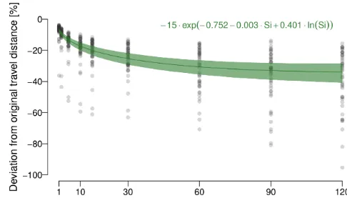
There is strong support that the expected deviation from the true distance follows an exponential function (Fig. 4), in-dicating that the relative error increase is larger at shorter sampling intervals, as can be seen in Fig. 4 by the estimated expected error levelling off with increasing re-discretisation interval duration.
Figure 3.Deviation from original travel distance covered within
2 h (box plots illustrate the same descriptive statistics as described in the caption for Fig. 2), as revealed by applying different sampling intervals.
Figure 4.Expected deviation from the original travel distances (in
%) conditional on re-discretisation interval duration (in minutes). The solid green line shows the estimated expectation (the functional form is described by the function as given on the top right of the figure); the green area shows a point-wise 99 % uncertainty interval for this estimated conditional expectation.
3.3 Impact of states on deviation
Step length
Density
0 100 200 300 400
0.000 0.002 0.004 0.006 0.008 0.010 0.012 State 1 State 2 State 3
Turning angle (radians)
Density 0.0 0.1 0.2 0.3 0.4 0.5 0.6 0.7
− π − π 2 0 π2 π
State 1 State 2 State 3 ● ● ● ●●● ● ● ● ● ●● ● ● ● ● ● ●●●●●●● ● ● ● ●● ● ●● ●● ● ●● ● ● ● ● ● ● ●●●●● ● ● ● ● ● ● ● ● ● ● ● ● ● ● ● ● ● ● ● ● ● ● ● ● ● ● ● ●●●● ● ●●● ● ● ● ● ● ● ● ● ● ● ● ● ● ● ● ● ● ● ● ● ● ● ● ● ● ● ● ● ● ● ● ● ● ● ● ● ● ●● ● ●●●●●●● ●●●●●●●●● ●● ● ● ● ● ● ● ● ● ●●●● ●●●● ●● ●● ●● ● ●●●● ● ● ● ● ● ● ● ● ● ● ● ●●● ● ● ● ● ● ● ● ● ● ● ● ● ● ● ● ● ● ● ● ● ● ●● ● ● ●●● ● ● ●●● ● ● ● ● ● ● ● ● ● ● ● ● ● ● ● ● ● ● ● ●●●●●● ● ● ● ● ● ● ● ● ● ● ● ●● ● ● ● ● ● ● ● ● ● ● ● ● ● ● ● ● ● ● ● ● ● ● ● ● ● ● ● ● ● ●●●●● ● ● ● ●●●● ●●●● ● ● ●●● ●● ●● ● ●●●● ● ●● ● ● ● ● ●●●● ●● ● ● ● ● ● ● ● ● ● ● ● ● ● ● ● ●● ● ● ●●● ●●●●●● ● ●● ● ● ● ●● ● ● ● ● ● ●●● ● ● ● ● ● ● ● ●●● ● ● ● ● ● ● ● ● ● ● ● ● ● ● ● ●●●● ● ● ●●●●●●● ● ●●●●●●●●●●● ●●●● ●● ●● ●● ●● ●● ●● ●●● ● ● ● ● ● ● ● ● ● ● ●● ●●●●● ●●● ● ● ●●● ●●●● ●●●●●●● ●●● ● ● ● ● ●●●●●●●●●●●●●● ● ● ● ●●●●● ● ● ● ● ● ● ● ● ● ● ● ● ● ● ● ●●● ● ● ● ●●● ● ● ● ●●● ● ● ● ● ● ● ● ● ● ● ● ● ● ● ●●● ● ●●●●●●●●●●●● ●● ●● ● ● ●●●●● ● ● ● ● ● ● ● ● ● ● ● ● ● ●● ● ● ● ● ● ● ● ● ● ● ●●●● ● ●●●●●●●●●●●●●●●●●● ● ● ● ● ● ● ● ● ● ● ● ● ● ●● ●●● ● ●● ● ● ● ● ●●●●●● ● ● ● ● ● ● ● ●●●● ●●● ● ● ● ● ● ● ● ● ● ● ●●●●●●●● ● ● ● ● ● ● ●● ● ● ● ● ●● ● ● ● ● ● ● ● ●●●●●●●●●●●● ● ● ● ● ● ● ● ● ● ● ●●●●●●●● ● ●● ● ● ● ● ● ● ● ● ● ● ● ● ● ● ● ● ● ● ● ● ● ●●●●●● ●●●●●●●●● ●● ● ● ●●● ● ● ● ●●● ● ● ● ● ● ● ● ● ● ● ● ● ● ● ● ● ● ● ● ● ● ● ● ● ● ● ● ● ● ● ● ● ● ●●●●● ● ● ● ● ● ● ● ● ● ● ● ● ● ● ● ● ● ●●●● ● ● ● ● ●●● ● ● ● ● ● ●● ● ●●●●●● ● ● ●●●●●● ● ● ● ● ● ● ● ● ● ●●●●●●●●●●●●●●● ●● ● ● ●● ● ● ● ● ● ● ● ● ● ●●●●● ● ● ● ● ● ●●●●●●●● ● ● ●● ● ●●●●●●● ● ● ● ● ●● ● ● ●● ● ● ●●● ●●●●●● ● ● ● ● ● ● ● ● ● ● ● ● ● ● ● ● ● ● ● ● ●● ●● ●●● ● ● ●● ●● ● ● ●● ● ● ● ● ● ● ● ● ● ● ● ● ● ● ● ● ● ● ● ● ● ● ● ● ●● ● ● ● ● ● ● ● ● ● ●● ●● ●●● ● ● ● ● ● ● ●● ● ●●●● ● ● ● ●● ● ● ● ● ●● ● ● ●●●●●● ● ●● ● ●● ● ●●●●●●● ● ● ● ● ● ● ● ● ● ● ● ●● ● ● ● ● ● ● ● ● ●●● ● ● ●●●●● ●● ●
Figure 5.Results of the hidden Markov model estimation. Blue lines on the left and middle plots illustrate the densities for the “resting”
state 1, dark grey lines show densities for state 2 (slow velocities, i.e. small step lengths per 5 min interval, approximately uniform distributed turning angles) and red lines illustrate the densities for state 3 (higher velocities and higher density for straight movements). The dashed histograms show the overall empirical distributions. The right figure shows the 47 tracks, coloured according to the states to which the Viterbi algorithm (based on the hidden Markov model results) categorised them (xandyaxes are scaled such that each track can be seen in the maximal graphical solution; i.e. they are not equally scaled across the 47 plots).
4 Discussion
Results of our analysis of the DTD of Guinea baboons met the general expectation: the higher the frequency of posi-tions, the more trustworthy the movement paths (Nathan et al., 2008). The absolute average underestimate of DTDs
was found to be less than 7 % for 1 fix min−1and less than
35 % for 1 fix/120 min. However, it can reach up to a max-imum of 30 and 90 % if respective sampling frequencies of
1 fix min−1 or 1 fix 120 min−1are applied. The increase of
deviation from true DTDs followed an exponential function, indicating that the average relative error increase is larger at shorter sampling intervals than at larger ones, which is in agreement with findings from Rowcliffe et al. (2012). For in-stance, whether, in the case of the Guinea baboons, we use a 90 or a 120 min sampling interval would not make a rele-vant difference in underestimating DTDs. At least for Guinea baboons we now have a reliable estimate of average underes-timation of DTDs, which we can, for example, use as a cor-rection when calculating absolute travel costs. We assume that similar magnitudes of underestimation of DTDs apply for other terrestrial primates, such as other baboon species.
The magnitude of error, however, is also dependent on the behaviour of the individuals under consideration. In the ex-treme, if an animal does not move over a long period, the true travelled distance is 0 and the deviation from the true value
Figure 6.Deviation from original travel distance by the artificial
5 min sampling scheme, conditional on the states as estimated by the Viterbi algorithm applied on the hidden Markov model results shown in Fig. 5. Box plots illustrate the same descriptive statistics as described in the caption for Fig. 2, with values of the median con-ditional deviations given directly in the figure, and also illustrated by crosses.
quickly with a lot of meandering. In our study, we analysed the impact of movement behaviour exemplarily at a 5 min sampling interval. As expected, in state 1 (mainly resting) the deviation was minimal, whereas it increased minimally if the animal moved slowly (state 2) and increased more if it moved quickly (state 3). Since the spatial behaviour of ba-boons and other animals is often influenced by ecological condition (e.g. temporal and spatial distribution of food), one can expect season might affect step length and path tortuosity (Calenge et al., 2009; Owen-Smith et al., 2010).
Moreover, the time of day might play an additional role in shaping the characteristics of a travel path. In Chacma
ba-boons (Papio ursinus), for example, Noser and Byrne (2010)
found that their study group used two different strategies over the course of the day to exploit available fruit trees. In the early morning, the baboons showed a more goal-directed travel behaviour with linear travel routes and high movement speeds, whereas the baboons travelled more opportunistically (slower and less directly) during the rest of the day. DTDs can also vary among seasons if the spatial distribution of re-sources changes and forces individuals to adapt their DTDs (Hemingway and Bynum, 2005). If such temporal patterns in movement behaviour are significant in a species, the estima-tion of error in DTDs needs to be adapted to these patterns.
We were able to determine underestimations of DTDs in a terrestrial primate, the Guinea baboon, when applying dif-ferent sampling intervals. The values of underestimation can be used as a corrective in estimations of absolute DTDs and travelling costs, which can make comparisons among differ-ent primate groups more reliable. Our analysis also showed, at least for terrestrial primates such as baboons, that there is no significant increase of underestimation beyond a sampling interval of 60 min (60, 90, 120 min). As shown in Fig. 4, this mainly results from a weaker increase in underestimation for larger interval durations, and less from an increase in estima-tion uncertainty. Such a priori knowledge on underestima-tions of DTDs is important to inform researchers conduct-ing GPS remote telemetry studies. Based on analyses such as ours, researchers can choose the “appropriate” sampling intensity in order to optimise the trade-off between sampling density and battery longevity.
We think that the overall magnitude of error, as found in our baboon study, will provide an estimate transferable also to other terrestrial or semi-terrestrial primate species. However, if the respective species show largely deviating movement behaviour, the magnitude of error will most likely change.
Data availability. Data are provided as Supplement S3.
The Supplement related to this article is available online at https://doi.org/10.5194/pb-4-143-2017-supplement.
Author contributions. DZ and MK designed the study. LD and
MK collected the data in the field. HS-R did most of the data anal-yses. LD, MK, HS-R and DZ wrote the paper.
Competing interests. The authors declare that they have no
con-flict of interest.
Acknowledgements. We thank the Diréction des Parcs
Na-tionaux and Ministère de l’Environnement et de la Protéction de la Nature de la République du Sénégal for permission to work in the Niokolo-Koba National Park (Attestation 0383/24/03/2009 and 0373/10/3/2012). In particular we thank the conservator of the Niokolo-Koba National Park for permitting and supporting this project research in the park. We also thank Vanessa Wilson for English language editing and two anonymous reviewers for their valuable comments. Funding was provided by the German Science Council DFG ZI 548/6-1 and the DAAD D/12/41834.
Edited by: Eberhard Fuchs
Reviewed by: two anonymous referees
References
Alfred, R., Ahmad, A. H., Payne, J., Williams, C., Ambu, L. N., How, P. M., and Goossens, B.: Home range and ranging behaviour of Bornean elephant (Elephas maximus borneensis) females, PLoS ONE, 7, e31400, https://doi.org/10.1371/journal.pone.0031400, 2012.
Blackwell, P. G., Niu, M., Lambert, M. S., and LaPoint, S. D.: Ex-act Bayesian inference for animal movement in continuous time, Methods Ecol. Evol., 7, 184–195, https://doi.org/10.1111/2041-210X.12460, 2016.
Bonnell, T. R., Henzi, S. P., and Barrett, L.: Sparse movement data can reveal social influences on individual travel decisions, arXiv 1511.01536, 2015.
Bradshaw, C. J. A., Sims, D. W., and Hays, G. C.: Measure-ment error causes scale-dependent threshold erosion of biolog-ical signals in animal movement data, Ecol. Appl., 17, 628–638, https://doi.org/10.1890/06-0964, 2007.
Bürkner, P. C.: brms: An R Package for Bayesian Multilevel Models using Stan, J. Stat. Softw., in press, 2017.
Cagnacci, F., Boitani, L., Powell, R. A., and Boyce, M. S.: Animal ecology meets GPS-based radiotelemetry: a perfect storm of op-portunities and challenges, Philos. T. R. Soc. B, 365, 2157–2162, https://doi.org/10.1098/rstb.2010.0107, 2010.
Calenge, C.: The package adehabitat for the R software: a tool for the analysis of space and habitat use by animals, Ecol. Model., 197, 516–519, https://doi.org/10.1016/j.ecolmodel.2006.03.017, 2006.
Calenge, C., Dray, S. and Royer-Carenzi, M.: The concept of ani-mals’ trajectories from a data analysis perspective, Ecol. Inform., 4, 34–41, https://doi.org/10.1016/j.ecoinf.2008.10.002, 2009. Chynoweth, M. W., Lepczyk, C. A., Litton, C. M., Hess, S.
island montane dry landscape, PLoS ONE, 10, e0119231, https://doi.org/10.1371/journal.pone.0119231, 2015.
Edelhoff, H., Signer, J., and Balkenhol, N.: Path segmentation for beginners: an overview of current methods for detect-ing changes in animal movement patterns, Mov. Ecol., 4, 21, https://doi.org/10.1186/s40462-016-0086-5, 2016.
Fleming, C. H., Calabrese, J. M., Mueller, T., Olson, K. A., Leimgruber, P., and Fagan, W. F.: From fine-scale foraging to home ranges: A semivariance approach to identifying movement modes across spatiotemporal scales, Am. Nat., 183, E154–E167, https://doi.org/10.1086/675504, 2014a.
Fleming, C. H., Calabrese, J. M., Mueller, T., Olson, K. A., Leimgruber, P., and Fagan, W. F.: Non-Markovian maximum likelihood estimation of autocorrelated movement processes, Methods Ecol. Evol., 5, 462–472, https://doi.org/10.1111/2041-210X.12176, 2014b.
Fleming, C. H., Fagan, W. F., Mueller, T., Olson, K. A., Leim-gruber, P., and Calabrese, J. M.: Estimating where and how animals travel: an optimal framework for path reconstruc-tion from autocorrelated tracking data, Ecology, 97, 576–582, https://doi.org/10.1890/15-1607.1, 2016.
Goffe, A. S., Zinner, D., and Fischer, J.: Sex and friendship in a multilevel society: behavioural patterns and associations between female and male Guinea baboons, Behav. Ecol. Sociobiol., 70, 323–336, https://doi.org/10.1007/s00265-015-2050-6, 2016. Gregory, T., Mullett, A., and Norconk, M. A.: Strategies for
navi-gating large areas: A GIS spatial ecology analysis of the bearded saki monkey,Chiropotes sagulatus, in Suriname, Am. J. Prima-tol., 76, 586–595, https://doi.org/10.1002/ajp.22251, 2014. Grueter, C. C., Li, D., van Schaik, C. P., Ren, B., Long, Y., and Wei,
F.: Ranging ofRhinopithecus bietiin the Samage Forest, China. I. Characteristics of range use, Int. J. Primatol., 29, 1121–1145, https://doi.org/10.1007/s10764-008-9299-9, 2008.
Hampson, B. A., De Laat, M. A., Mills, P. C., and Pollitt, C. C.: Distances travelled by feral horses in “outback” Australia, Equine Vet. J., 42, 582–586, https://doi.org/10.1111/j.2042-3306.2010.00203.x, 2010.
Harris, K. J. and Blackwell, P. G.: Flexible continuous-time mod-elling for heterogeneous animal movement, Ecol. Modell., 255, 29–37, https://doi.org/10.1111/2041-210X.12460, 2013. Hemingway, C. A. and Bynum, N.: The influence of seasonality on
primate diet and ranging, in: Seasonality in Primates Studies of Living and Extinct Human and Non-Human Primates, edited by: Brockman, D. K. and van Schaik, C. P., Cambridge University Press, Cambridge, 57–104, 2005.
Hoffman, T. S. and O’Riain, M. J.: Troop size and human-modified habitat affect the ranging patterns of a chacma baboon population in the Cape Peninsula, South Africa, Am. J. Primat., 74, 853– 863, https://doi.org/10.1002/ajp.22040, 2012.
Isbell, L. A. and Bidner, L. R.: Vervet monkey (Chlorocebus pygery-thrus) alarm calls to leopards (Panthera pardus) function as a predator deterrent, Behaviour, 153, 591–606, 2016.
Johnson, C., Piel, A. K., Forman, D., Stewart, F. A., and King, A. J.: The ecological determinants of baboon troop move-ments at local and continental scales, Mov. Ecol., 3, 14, https://doi.org/10.1186/s40462-015-0040-y, 2015.
Kays, R., Crofoot, M., Jetz, W., and Wikelski, M.: Terrestrial an-imal tracking as an eye on life and planet, Science 348, 1222, https://doi.org/10.1126/science.aaa2478, 2015.
Laube, P. and Purves, R. S.: How fast is a cow? Cross-scale analysis of movement data, T. GIS, 15, 401–418, https://doi.org/10.1111/j.1467-9671.2011.01256.x, 2011. Laundré, J. W., Reynolds, T. D., Knick, S. T., and Ball, I. J.:
Ac-curacy of daily point relocations in assessing real movement of radio-marked animals, J. Wildlife Manage., 51, 937–940, https://doi.org/10.2307/3801763, 1987.
Markham, A. C. and Altmann, J.: Remote monitoring of primates using automated GPS technology in open habitats, Am. J. Prima-tol., 70, 495–499, https://doi.org/10.1002/ajp.20515, 2008. Michelot, T., Langrock, R., and Patterson, T. A.: moveHMM: an R
package for the statistical modelling of animal movement data using hidden Markov models, Methods Ecol. Evol., 7, 1308– 1315, https://doi.org/10.1111/2041-210X.12578, 2016. Mills, K. J., Patterson, B. R., Murray, D. L., and Bowman, J.: Effects
of variable sampling frequencies on GPS transmitter efficiency and estimated wolf home range size and movement distance, Wildlife Soc. B., 34, 1463–1469, https://doi.org/10.2193/0091-7648(2006)34[1463:EOVSFO]2.0.CO;2, 2006.
Naha, D., Jhala, Y. V., Qureshi, Q., Roy, M., Sankar, K., and Gopal, R.: Ranging, activity and habitat use by tigers in the mangrove forests of the Sundarban, PLoS ONE, 11, e0152119, https://doi.org/10.1371/journal.pone.0152119, 2016.
Nathan, R., Getz, W. M., Revilla, E., Holyoak, M., Kad-mon, R., Saltz, D., and Smouse, P. E.: A movement ecology paradigm for unifying organismal movement re-search, P. Natl. Acad. Sci. USA, 105, 19052–19059, https://doi.org/10.1073/pnas.0800375105, 2008.
Noser, R. and Byrne, R. W.: How do wild baboons (Papio ursi-nus) plan their routes? Travel among multiple high-quality food sources with inter-group competition, Anim. Cogn., 13, 145– 155, https://doi.org/10.1007/s10071-009-0254-8, 2010. Osborne, P. E. and Glew, L.: Geographical information systems and
remote sensing, in: Field and Laboratory Methods in Primatol-ogy, edited by: Setchell, J. M. and Curtis, D. J., Cambridge Uni-versity Press, Cambridge, 69–89, 2011.
Owen-Smith, N., Fryxell, J. M., and Merrill, E. H.: For-aging theory upscaled: the behavioural ecology of herbi-vore movement, Philos. T. R. Soc. B, 365, 2267–2278, https://doi.org/10.1098/rstb.2010.0095, 2010.
Patzelt, A., Kopp, G. H., Ndao, I., Kalbitzer, U., Zinner, D., and Fischer, J.: Male tolerance and male–male bonds in a multilevel primate society, P. Natl. Acad. Sci. USA, 111, 14740–14745, https://doi.org/10.1073/pnas.1405811111, 2014.
Pebsworth, P. A., Morgan, H. R., and Huffman, M. A.: Evaluat-ing home range techniques: use of Global PositionEvaluat-ing System (GPS) collar data from chacma baboons, Primates, 53, 345355, https://doi.org/10.1007/s10329-012-0307-5, 2012a.
Pebsworth, P. A., MacIntosh, A. J. J., Morgan, H. R., and Huffman, M. A.: Factors influencing the ranging behav-ior of chacma baboons (Papio hamadryas ursinus) living in a human-modified habitat, Int. J. Primatol., 33, 872–887, https://doi.org/10.1007/s10764-012-9620-5, 2012b.
Postlethwaite, C. M. and Dennis, T. E.: Effects of temporal resolu-tion on an inferential model of animal movement, PLoS ONE, 8, e57640, https://doi.org/10.1371/journal.pone.0057640, 2013. Ren, B., Li, M., Long, Y., Grueter, C. C., and Wei, F.:
methodological consideration, Int. J. Primatol., 29, 783–794, https://doi.org/10.1007/s10764-008-9251-z, 2008.
Ren, B., Li, M., Long, Y., and Wei, F.: Influence of day length, am-bient temperature, and seasonality on daily travel distance in the Yunnan snub-nosed monkey at Jinsichang, Yunnan, China, Am. J. Primatol., 71, 233–241, https://doi.org/10.1002/ajp.20641, 2009.
Reynolds, T. D. and Laundre, J. W.: Time intervals for estimating pronghorn and coyote home ranges and daily movements, J. Wildlife Manage., 54, 316–322, https://doi.org/10.2307/3809049, 1990.
Rowcliffe, J. M., Carbone, C., Kays, R., Kranstauber, B., and Jansen, P. A.: Bias in estimating animal travel distance: the ef-fect of sampling frequency. Methods Ecol. Evol., 3, 653–662, https://doi.org/10.1111/j.2041-210X.2012.00197.x, 2012. Santhosh, K., Kumara, H. N., Velankar, A. D., and Sinha, A.:
Rang-ing behavior and resource use by lion-tailed macaques (Macaca silenus) in selectively logged forests, Int. J. Primatol., 36, 288– 310, https://doi.org/10.1007/s10764-015-9824-6, 2015. Sarma, K. and Kumar, A.: The day range and home range
of the eastern hoolock gibbon Hoolock leuconedys (Mam-malia: Primates: Hylobatidae) in Lower Dibang Valley District in Arunachal Pradesh, India, J. Threat. Taxa, 8, 8641–8651, https://doi.org/10.11609/jott.2739.8.4.8641-8651, 2016. Shamoun-Baranes, J., van Loon, E. E., Purves, R. S.,
Speck-mann, B., Weiskopf, D., and Camphuysen, C. J.: Analysis and visualization of animal movement, Biol. Lett., 8, 6–9, https://doi.org/10.1098/rsbl.2011.0764, 2011.
Sprague, D. S., Kabaya, H., and Hagihara, K.: Field testing a global positioning system (GPS) collar on a Japanese monkey: reliabil-ity of automatic GPS positioning in a Japanese forest, Primates, 45, 151–154, https://doi.org/10.1007/s10329-003-0071-7, 2004.
Stan Development Team: Stan: A C++Library for Probability and Sampling, Version 2.10.0, available at: http://mc-stan.org/ (last access: 1 July 2016), 2015.
Stark, D. J., Vaughan, I. P., Ramirez Saldivar, D. A., Nathan, S. K. S. S., and Goossens, B.: Evaluating methods for estimat-ing home ranges usestimat-ing GPS collars: A comparison usestimat-ing pro-boscis monkeys (Nasalis larvatus), PLoS ONE, 12, e0174891, https://doi.org/10.1371/journal.pone.0174891, 2017.
Sterling, E. J., Bynum, N., and Blair, M. E. (Eds.): Primate Ecology and Conservation, A Handbook of Techniques, Oxford Univer-sity Press, Oxford, 2013.
Strandburg-Peshkin, A., Farine, D. R., Couzin, I. D., and Crofoot, M. C.: Shared decision-making drives collec-tive movement in wild baboons, Science, 348, 1358–1361, https://doi.org/10.1126/science.aaa5099, 2015.
Vehtari, A., Gelman, A., and Gabry, J.: Practical Bayesian model evaluation using leave-one-out cross-validation and WAIC, Stat. Comput., 27, 1413, https://doi.org/10.1007/s11222-016-9696-4, 2016.