Conjugate Gradient Methods for Computing Weighted Analytic Center for Linear Matrix Inequalities Using Exact and Quadratic Interpolation Line Searches

(1)

http://www.sciencepublishinggroup.com/j/ajam doi: 10.11648/j.ajam.20200801.11

ISSN: 2330-0043 (Print); ISSN: 2330-006X (Online)

Conjugate Gradient Methods for Computing Weighted

Analytic Center for Linear Matrix Inequalities Using Exact

and Quadratic Interpolation Line Searches

Shafiu Jibrin

*

, Ibrahim Abdullahi

Department of Mathematics, Faculty of Science, Federal University, Dutse, Jigawa State, Nigeria

Email address:

*

Corresponding author

To cite this article:

Shafiu Jibrin, Ibrahim Abdullahi. Conjugate Gradient Methods for Computing Weighted Analytic Center for Linear Matrix Inequalities Using Exact and Quadratic Interpolation Line Searches. American Journal of Applied Mathematics. Vol. 8, No. 1, 2020, pp. 1-10.

doi: 10.11648/j.ajam.20200801.11

Received: October 18, 2019; Accepted: November 27, 2019; Published: January 4, 2019

Abstract:

We study the problem of computing the weighted analytic center for linear matrix inequality constraints. In this paper, we apply conjugate gradient (CG) methods to find the weighted analytic center. CG methods have low memory requirements and strong local and global convergence properties. The methods considered are the classical methods by Hestenes-Stiefel (HS), Fletcher and Reeves (FR), Polak and Ribiere (PR) and a relatively new method by Rivaie, Abashar, Mustafa and Ismail (RAMI). We compare performance of each method on random test problems by observing the number of iterations and time required by the method to find the weighted analytic center for each test problem. We use Newton’s method exact line search and Quadratic Interpolation inexact line search. Our numerical results show that PR is the best method, followed by HS, then RAMI, and then FR. However, PR and HS performed about the same with exact line search. The results also indicate that both line searches work well, but exact line search handles weights better than the inexact line search when some weight is relatively much larger than the other weights. We also find from our results that with Quadratic interpolation line search, FR is more susceptible to jamming phenomenon than both PR and HS.

Keywords:

Linear Matrix Inequalities, Weighted Analytic Center, Semidefinite Programming, Conjugate Gradient Methods

1. Introduction

We consider the following system of linear matrix inequality constraints:

( )

( ) ( )

0 1

( ) : 0, ( 1, 2,..., )

n j

j j

i i i

A x A x A j q

=

= +

∑

= (1)

where x ∈ IRn _{is a variable and each} ( )j i

A is mj x mj symmetric matrix.

LMI constraints have applications in engineering, geometry, statistics and in the field of semidefinite programming ([1-6]). Let R_{denote the feasible region defined by the inequalities}

(1). We will assume that the feasible region R_{is bounded}

and it has a nonempty interior.

Given ω > 0, the weighted analytic centered for the system

(1) is optimal solution of the optimization problem ([7-9]):

min{φω(x) | x ∈ IRn} where,

( ) 1

1

[( ( )) ] ( )

( )

otherwise

q

j j

j

logdet A x if x int x

ω ω

φ ₌ −



∈ 

=  ∞ 

∑

R

(2)

In the special case of linear constraints, weighted analytic center has been studied extensively in the past (for example, [10]). A weighted analytic center for LMIs which extends the definition given in [10] was given in [7, 8].

(2)

method can also be used to compute the weighted analytic center given a starting interior point [7]. Newton’s method requires the gradient and Hessian of the objective function φω(x) or the Jacobian of a residual function. In this paper, we give conjugate gradient (CG) methods for finding the weighted analytic center starting from a given interior point. CG methods use only the gradient of φω(x) and do not require the Hessian of φω(x). This approach is particularly beneficial when the dimensions mj of the matrices are high. CG methods also have low memory requirements and strong local and global convergence properties [14].

In this work, we focus on four conjugate gradient methods The methods considered are the classical methods by Hestenes-Stiefel (HS), Fletcher and Reeves (FR), Polak and Ribiere (PR) discussed in [14] and a relatively new method by Rivaie, Abashar, Mustafa and Ismail (RAMI) [15]. We compare performance of each method on random test problems by observing the number of iterations and time required by the method to find the weighted analytic center for each test problem. We use Newton’s method exact line search and Quadratic Interpolation inexact line search.

2. Conjugate Gradient Methods

Consider a continuously differentiable function f: Rn → IR and the following unconstrained optimization problem

min{f(x): x ∈ Rn}. (3) Let g(x) denote the gradient of f(x). A conjugate gradent method to find a solution to problem 3 works as follows. Given an initial guess xo∈ Rn, a sequence {xk} is generated by:

1

k k k k

x ₊ =x +α d (4) and the direction dk is defined as

1

0, 1,

k k

k k k g if k d

g

β

d if k +

+

− =

 =

− + ≥

 (5)

where xk is the current iterate, gk =g(xk), βk is the CG coefficient and αk > 0 is the step-length obtained by a line search. A common convergence criterion for a CG method is

( )

g xk ≤TOL, where TOL is a given tolerance.

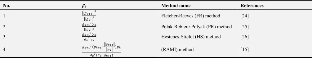
Over the years, a variety of CG formulas were given, where majorly, differences are in the parameter βk. The work by [13] discussed details on some CG methods with special emphasis on their global convergence. In recent times, research carried out by [16-23, 15] focused on some modified CG methods. The summary of the CG methods considered in this work are given in the Table 1, where ||.|| denotes the Euclidean norm.

Table 1. The classical formulas for parameter βk.

No. βk Method name References

1 |_{| |}| Fletcher-Reeves (FR) method [24]

2 _{|| ||} Polak-Rebiere-Polyak (PR) method [25]

3 Hestenes-Stiefel (HS) method [26]

4 ( )

( )

(RAMI) method [15]

For convex quadratic problems, the first three methods in Table 1 are equivalent using exact line search to compute the step length α, but behave differently if the objective function f(x) is non-convex. The classical method FR possess strong convergence properties but not computationally powerful. While, methods like PR and HS perform better computationally, but may not always converge. Problems associated with classical methods gave room for improvement through modification and hybridization. Convergence analysis and numerical experiments showed that RAMI method proposed by [15] is robust as compared to FR and PR, since it solved all the

benchmark problems under consideration, while FR and PR did not.

In this research, these four CG methods are employed to find weighted analytic centers for the system (1), observe and compare their computational strengths.

The gradient g of the barrier function φω(x) is given by [8]:

( ) 1 ( )

1

( ) ( ) ( ( )) ? , ( 1, , )

q

j j

i i j i

j

g x φ_ω x ω A x − A i n

=

= ∇ = −

∑

= … (6)

The Hessian H(x) of φω(x) is given by [8]:

( ) 1 ( ) ( ) 1 ( )

1

( ) [( ( )) ] ?[( ( )) ], ,( 1, , )

q

k k T k k

ij k i j

k

H x ω A x − A A x − A i j n

=

∑

= … (7)

3. Line Searches for Our Conjugate

Gradient Methods

We find exact and inexact step-sizes for our conjugate gradient methods. Newton’s method is used to find the

exact step-size and inexact step-size is found using Quadratic interpolation. We also discuss convergence for the methods.

Let x be an interior point of R_{, then} ( )

( ) 0

j

A x ≻ for each constraint j, and the square root of A(j)_{(x) exists. Given}

(3)

1 1

2 2

( ) ( ) ( )

1

( , ) ( ) ( ) ( ) , (1 )

n

j j j

j i i

i

B d x A x− d A A x − j q

=

= −

∑

≤ ≤

Consider the objective barrier function φω(x). Let dk be a conjugate direction generated by the CG algorithm at the current iterate xk. Let h(α) = φω(xk + αdk). The exact step-size αk is given by

αk = argmin{h(α) | α ≥ 0}. (8) The following results reduces the cost of computing the exact stepsize using Newton’s method.

Theorem 1 Let xk be an interior point of R and be the ith eigenvalue of Bj(dk, xk). Then

( ) ( )

1 1 1

( ) ( ( )) (1 )

j

m

q q

j j

j k j i

j j i

hα ω logdet A x ω log αλ

= = =

= −

∑

−

∑ ∑

+ (9)

Proof:

( ) 1

1 ( ) 1 ( ) ( ) 0 1 1 ( ) ( ) ( ) 0 1

( )

(

)

=

log det[(

(

)) ]

= -

logdet[

(

)]

= -

logdet[

(

)

]

= -

logdet[

( )

(

)

j

w k k

q

j

j k k

j q

j

j k k

j

m q

j j

j k k i i

j i

m

j j j

j k i i k i i

i i

h

x

d

w

A

x

d

w

A

x

d

w

A

x

d

A

w

A

x

A

d

A

α φ

α

− = = = = =

=

+

∑

1 2

1 1 1

2 2 2

1 1 ( ) 1 ( ) ( ) ( ) ( ) 1 ( ) ( )

]

= -

logdet[

( )

(

,

)]

logdet[

( ) (

=

( )

(

,

)

( ) )

( ) ]

[logdet(

( )) logdet(

=

(

j m q j q j

j k j k k

j

j q

j k

j j j

j _k _j _k _k _k _k

j

j k

j

w

A

x

B d x

w

A

x

I

A

x

B d x A

x

A

x

w

A

x

I

A

α

= = = − − =

+

∑

1 1

2 ( ) 2

1

( ) ( )

1 1

( ) ( )

1 1 1

)

(

,

)

( ) ]

[logdet(

( ))

(1

)]

logdet(

( ))

log(1

)]

j

q

j

j k j k k k

m q

j j

j k i

j i

m

q q

j j

j k j i

j j i

x

B d x A

x

w

A

x

w

A

x

w

αλ

− − = = = = = =

= −

+

= −

−

+

∑

∑ ∑

Corollary 1 The derivatives of h(α) are given by

( ) ' ( ) 1 1 ( ) -(1 ) j m q j i j _j i j i

h α w λ

αλ = = =

+

∑ ∑

(10)

2 ( ) '' ( ) 1 1 ( ) 1 j m q j i j _j i j i

h α w λ

αλ = =   = _ _ +  

∑ ∑

(11)

Exact line search is applied to compute the step-size αk (8) in our CG algorithms using one-dimensional Newton’s method starting from α = 0:

' 1 _'' ( ) ( ) k k k k h h

α

+ = − (12)

We will need the following result to approximate the step-size αk (8) using Quadratic interpolation. The proof of Theorem 2 can be found in [27].

Denote the largest positive eigenvalue of a symmetric matrix B by λ+max(B).

Theorem 2 Let xk be an interior point ofR. Assume the ray

{xk +σdk | σ ≥ 0} intersects the boundary of A( )j ( )x 0 at

the point x_k+

σ

₊( )j d_k. Then, the distance to the boundary along the ray from xk is given by

( )

1 / ( ( , ))

j

max B dj k xk

σ λ+

+ = (13)

Proof: A( )j ( )x ≻0 when x is in the interior ofR_{, but on}

the boundary it must have at least one zero eigenvalue. Then

{

}

( )j _min _| _{0, det[} ( )j ₍ _)] ₀

k k

A x d

σ₊ = µ µ> +µ = (14)

Now, when µ>0

( ) ( ) ( )

1

det[ ( )] 0 det[ ( ) ( ) ] 0

n

j j j

k k k k i i

i

A x µd A x µ d A

= + = ⇔ +

∑

= 1 1 2 2 ( ) ( ) 1 1

det[ ( ) ( ( ) ( ) ] 0

n

j j

k k i i k

i

I A x d A x

µ − ₌ −

⇔ +

∑

=

1

det[ I B d_j( _k,x_k)] 0 µ

⇔ − =

1

is an eigenvalue of B d_j( _k,x_k) µ

⇔

1 is an eigenvalue of B d_j( _k,x_k)

µ −

⇔

This and (14) give

( )

1 / ( ( , ))

j

max B dj k xk

σ λ+

+ =

(4)

{

( )

}

min j | 1 j q

σ₊= σ₊ ≤ ≤ (15)

where

σ

₊( )j is given by (13). Note that σ+ exists since R is

bounded and xk is an interior point of R.

The following describes Quadratic interpolation line search for approximating the step-sze αk (8) in our CG algorithms (see [28]).

Quadratic Interpolation

Step 1: Use (15) to find the distance σ+ from xk to the boundary of the bounded feasible region R_{in the direction}

dk

Step 2: Set α1 = 0 and α3 = σ+

Step 3: Consider h(α) = φω(xk + αdk) Repeat

3 3/ 2 α =α

3 1

Until (hα )<h(α ) Let α2 = α3/2

Step 4: Compute the zero of the quadratic polynomial P (α) passing through the points (α1, P(α1)), (α2, P(α2)) and (α3,

P(α3)). The zero is given by

(

1

)

3

*

2 1 2

h h

α = α −

where,

2 1

1

2 1

3 2

2

3 2 2 1 3

3 1

( ) ( )

. h h h

h h h

α α

α α − =

− − =

−

Step 5: If α3 < α∗

set αk = α3

else set αk = α∗ end

Let x0 be a starting point for the CG method and consider

the level set

L_{= {x}∈_IRn

| g(x) ≤ g(x0)}

The gradient g(x) = ∇φω(x) is called Lipschitz continuous in a neighborhood N _ofL_{if there exists K ≥ 0 such that}

( ) ( ) , .

g x −g y ≤K x−y ∀x y∈N

L _{is called} _bounded _{if there is} _{r >} _{0 such that}

x ≤ ∀ ∈r x L_.

Let xk be the sequence generated by the CG method. The method is called globally convergent if g x( _k) =0 for some k or lim_k_→inf₀ xk =0.

If the gradient g(x) = ∇φω(x) is Lipschitz continuous in a neighborhood of L_{, FR method with exact line search is}

globally convergent [29]. We are not aware of any implementation or convergence analysis for FR with Quadratic interpolation inexact line search in the literature. FR is known to be susceptible to jamming phenomenon where it takes many short steps without significant decrease in the objective function φω(x) [14].

PR is globally convergent when φω(x) is strongly convex and the line search is exact [30]. PR and HS method with exact line search coincide and each is globally convergent if xk+1−xk converges to 0 and g is Lipschitz continuous in a neighborhood of L _{[31]. Again, we have not seen any}

implementation or convergence analysis for either PR or HS with Quadratic interpolation inexact line search in the literature. Both PR and HS are less susceptible to jamming phenomenon than FR [14].

RAMI conjugate method with exact line search is globally convergent if g is Lipschitz continuous in a neighborhood of

L _and L _{is bounded [15]. We are not aware of any}

implementation or convergence analysis for RAMI with Quadratic interpolation inexact line search in the literature.

The level set L _{is bounded since} L⊆R _and R_is

bounded. Theorem 3 and Theorem 4 show that the conjugate gradient methods with exact line search applied to our weighted analytic center problem are globally convergent. They show that the methods are suitable.

Theorem 3 The barrier function φω(x) is strongly convex

over the interior of the feasible region R.

Proof: The assumption that R_{is bounded and it has a}

nonempty interior implies that the function φω(x) is strictly

convex over R_{[8]. Hence, the Hessian H(x) (2) of φ}_ω_{(x) has}

positive eigenvalues in the interior of R_{. Since} R_is

bounded, the smallest eigenvalue must have a positive minimum value γ. So, H x( ) γI in the interior of R_{. This}

and the fact that φω(x) is twice differentiable ([27]) means that

φω(x) is strongly convex in the interior of R.

Theorem 4 The gradient g(x) = ∇φω(x) is Lipschitz

continuous in a neighborhood of the level set L_{= {x}_∈_IRn_|

g(x) ≤ g(x0)}.

Proof: By [27], φω(x) is analytic in the interior of R. So,

g(x) = ∇φω(x) is also analytic in the interior ofR. Choose any

neighborhood N _ofL_.N _{is bounded since} N ⊆ ⊆L R

and R_{is bounded. Let f(t) = g((1 − t)x + ty. By the mean}

value theorem, for some c ∈ (0, 1)

g(y) − g(x) = f(1) − f(0) = f0(c) = ∇g((1 − c)x + cy) • (y − x) By Cauchy-Schwartz’s inequality,

.

| ( ) ( ) | | ((1 ) ) ( ) |

((1 ) ) .

g y g x g c x cy y x g c x cy y x

− = ∇ − + −

≤ ∇ − + −

Since N _{is bounded and}∇_g_{is continuous on} N _{, there}

exists K ≥ 0 such that

(5)

Hence, g(x) is Lipschitz continuous in N _.

4. Numerical Experiments

In this section, we present numerical experiments to compare HS, FR, HR and RAMI conjugate gradient methods using exact and interpolation line searches.

All numerical experiments were done using a Lenevo-PC computer with codes written in MATLAB version 8. In all of the

problems, each LMI 0( ) ( ) 1

0 n

j j

i i i

A x A

=

+

∑

was generated as

follows: A₀( )j is an mj × mj diagonal matrix with each diagonal entry chosen from U(0, 1) distribution. Each A_i( )j (1≤ ≤i n) is a random mj × mj symmetric sparse matrix with approximately 0.8 ∗ m2j nonzero entries generated using the Matlab command

sprandsym(mj, 0.8). This ensures that each of our test problems is random, and that the origin is an interior point for each test problem. HS, FR, PR and RAMI congujate gradient methods were applied to each problem using a maximum of 1000 iterations and a tolerance TOL = 10−4_{. Each method is stopped}

after 1000 iteration or if g x( _k) ≤TOL.

Table 2 gives the list of test problems. The second column of the table is ambient dimension n and the third column gives the number q of LMI constraints. The sizes [m1,...,mq] of the matrices is given in the fourth column.

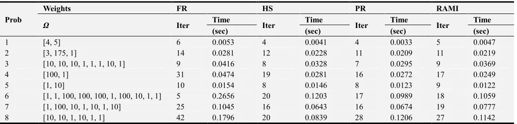
Table 3 gives the number of iteration and time (in seconds) taken by each method to find the weighted analytic center for the given weights using exact line search. The exact line search was done using one-dimensional Newton’s method.

Table 2. Test Problems.

LMI Test Problem n q [m1,...,mq]

1 2 2 [1, 2]

2 2 3 [5, 4, 5]

3 2 8 [2, 4, 5, 5, 5, 1, 5, 4]

4 3 2 [5, 4]

5 3 2 [3, 4]

6 4 10 [4, 5, 1, 4, 2, 3, 5, 5, 2, 1]

7 4 7 [2, 4, 4, 5, 4, 2, 1]

8 5 6 [5, 1, 4, 4, 4, 5]

9 5 4 [4, 1, 5, 1]

10 6 3 [4, 1, 5]

11 6 8 [2, 5, 2, 5, 5, 3, 5, 2]

12 7 2 [5, 4]]

13 7 4 [1, 4, 1, 2]

14 8 5 [1, 1, 4, 3, 3]

15 8 5 [5, 4, 5, 2, 5]

16 9 3 [3, 2, 5]

17 9 3 [5, 4, 4]

18 10 8 [4, 2, 3, 4, 5, 4, 4, 2]

19 10 8 [4, 5, 3, 5, 4, 2, 2, 4]

20 10 9 [5, 2, 5, 3, 2, 1, 3, 2, 2]

21 3 6 [3, 4, 1, 5, 4, 1]

22 5 7 [2, 3, 5, 5, 2, 4, 2]

23 5 3 [5, 5, 2]

24 5 9 [2, 4, 4, 1, 4, 5, 3, 5, 1]

25 10 3 [1, 5, 2]

26 5 10 [3, 4, 1, 3, 1, 4, 4, 5, 4, 4]

27 3 7 [2, 3, 4, 5, 4, 1, 5]

28 5 7 [2, 3, 5, 5, 2, 4, 2]

29 3 8 [5, 3, 3, 5, 5, 4, 2, 3]

30 2 6 [4, 4, 3, 1, 5, 2]

Table 3. Iterations and time taken by each method to find the weighted analytic center for the given weights using exact line search (Newton’s method).

Prob

Weights FR HS PR RAMI

Ω Iter Time Iter Time Iter Time Iter Time

(sec) (sec) (sec) (sec)

1 [4, 5] 6 0.0053 4 0.0041 4 0.0033 5 0.0047

2 [3, 175, 1] 14 0.0281 12 0.0228 11 0.0209 11 0.0219

3 [10, 10, 10, 1, 1, 1, 10, 1] 9 0.0416 8 0.0328 7 0.0295 9 0.0369

4 [100, 1] 31 0.0474 19 0.0281 16 0.0272 17 0.0249

5 [1, 10] 10 0.0154 8 0.0146 8 0.0123 9 0.0122

6 [1, 1, 100, 100, 100, 1, 100, 10, 1, 1] 5 0.2656 20 0.1203 17 0.0989 18 0.1059

7 [1, 100, 10, 1, 10, 1, 10] 25 0.1045 16 0.0643 16 0.0674 19 0.0777

(6)

Prob

Weights FR HS PR RAMI

(sec) (sec) (sec) (sec)

9 [100, 1, 1, 1] 107 0.2857 49 0.1328 48 0.1304 137 0.3728

10 [10, 1, 100] 20 0.0517 19 0.0444 21 0.0482 23 0.0537

11 [1, 1, 1, 10, 10, 1, 100, 1] 46 0.2458 25 0.1315 24 0.1257 31 0.1646

12 [1, 10] 47 0.0912 36 0.0682 34 0.0644 53 0.1011

13 [1, 10, 1, 100] 52 0.1467 35 0.0989 38 0.1063 64 0.1797

14 [1, 1, 10, 10, 10] 34 0.1317 34 0.1321 35 0.1314 42 0.1594

15 [10, 10, 1, 1, 100] 90 0.3723 37 0.1528 24 0.1006 49 0.2001

16 [10, 1, 1] 209 0.5898 73 0.2014 71 0.2052 268 0.750

17 [100, 100, 1] 70 0.1941 56 0.1546 41 0.1146 76 0.2110

18 [10, 1, 1, 1, 10, 10, 1, 1] 48 0.3132 27 0.1725 29 0.1874 30 0.1951

19 [1, 10, 1, 100, 1, 10, 10, 1] 177 1.1595 33 0.2144 33 0.2177 46 0.3010 20 [1, 10, 10, 1, 1, 1, 1, 1, 100] 85 0.6547 38 0.2885 46 0.3509 61 0.4712

21 [1, 1, 1, 1, 10, 1] 38 0.1313 16 0.0538 11 0.0385 11 0.0366

22 [10, 1, 1, 1, 10, 1, 1] 18 0.0801 15 0.0659 13 0.0642 16 0.0679

23 [100, 1, 1] 22 0.0479 27 0.0617 27 0.0621 25 0.0569

24 [100, 1, 100, 100, 100, 10, 1, 1, 10] 35 0.2086 20 0.1149 19 0.1089 23 0.1306

25 [1, 100, 10] 61 0.1757 65 0.1887 59 0.1707 132 0.3827

26 [7, 7, 7, 8, 7, 6, 4, 106_{, 3, 6]} ₈₇ _0.6418 ₉₂ _0.6529 ₇₉ _0.5501 ₁₇₇ _1.2600

27 [3, 5, 2, 1, 106_{, 2, 7]} ₄₃ _0.2032 ₃₇ _0.1607 ₃₂ _0.1516 ₅₃ _0.2383

28 [1, 1, 4, 8, 5, 8, 3, 106_] ₄₂ _0.2234 ₃₅ _0.1906 ₃₇ _0.2048 ₃₂ _0.1697

29 [2, 106_{, 4, 3]} ₃₂ _0.0952 ₃₃ _0.0919 ₁₈ _0.0535 ₂₉ _0.0802

30 [4, 6, 5, 3, 106_{, 4]} ₁₃ _0.0464 ₈ _0.0267 ₈ _0.0315 ₉ _0.0291

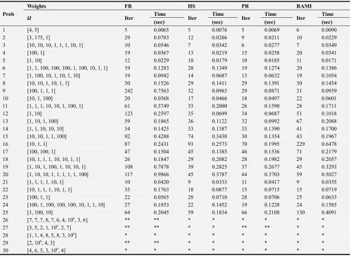
Table 4. Iterations and time taken by each method to find the weighted analytic center for the given weights using inexact line search (Quadratic Interpolation). The entry “⊻” means that CG method has failed to find the weighted analytic center due to numerical problems and “⊻ ⊻” if it failed after the maximum number of 1000 iterations (jamming phenomenon).

Prob

Weights FR HS PR RAMI

(sec) (sec) (sec) (sec)

1 [4, 5] 5 0.0065 5 0.0076 5 0.0069 6 0.0090

2 [3, 175, 1] 29 0.0783 12 0.0266 9 0.0211 10 0.0229

3 [10, 10, 10, 1, 1, 1, 10, 1] 10 0.0546 7 0.0342 6 0.0277 7 0.0349

4 [100, 1] 19 0.0367 13 0.0219 15 0.0258 20 0.0341

5 [1, 10] 12 0.0229 10 0.0179 10 0.0185 11 0.0171

6 [1, 1, 100, 100, 100, 1, 100, 10, 1, 1] 19 0.1283 20 0.1349 19 0.1274 20 0.1386

7 [1, 100, 10, 1, 10, 1, 10] 19 0.0942 14 0.0687 13 0.0632 19 0.1054

8 [10, 10, 1, 10, 1, 1] 30 0.1526 29 0.1411 29 0.1391 30 0.1454

9 [100, 1, 1, 1] 242 0.7563 32 0.0963 29 0.0871 31 0.0939

10 [10, 1, 100] 20 0.0568 17 0.0466 18 0.0497 22 0.0601

11 [1, 1, 1, 10, 10, 1, 100, 1] 61 0.3749 33 0.2000 26 0.1590 28 0.1711

12 [1, 10] 123 0.2597 35 0.0699 34 0.0687 51 0.1018

13 [1, 10, 1, 100] 59 0.1865 36 0.1122 32 0.0992 67 0.2088

14 [1, 1, 10, 10, 10] 34 0.1425 33 0.1387 33 0.1390 41 0.1700

15 [10, 10, 1, 1, 100] 92 0.4288 74 0.3430 30 0.1354 43 0.1967

16 [10, 1, 1] 87 0.2431 93 0.2573 70 0.1995 229 0.6478

17 [100, 100, 1] 47 0.1504 45 0.1385 46 0.1536 71 0.2179

18 [10, 1, 1, 1, 10, 10, 1, 1] 26 0.1847 29 0.2082 28 0.1982 29 0.2057

19 [1, 10, 1, 100, 1, 10, 10, 1] 108 0.7878 39 0.2825 37 0.2677 45 0.3293 20 [1, 10, 10, 1, 1, 1, 1, 1, 100] 117 0.9866 45 0.3787 44 0.3703 59 0.5027

21 [1, 1, 1, 1, 10, 1] 10 0.0420 9 0.0333 11 0.0417 9 0.0355

22 [10, 1, 1, 1, 10, 1, 1] 35 0.1763 18 0.0877 15 0.0715 15 0.0719

23 [100, 1, 1] 22 0.0565 28 0.0710 28 0.0706 25 0.0633

24 [100, 1, 100, 100, 100, 10, 1, 1, 10] 27 0.1853 22 0.1452 19 0.1228 24 0.1583

25 [1, 100, 10] 64 0.2045 59 0.1834 66 0.2108 130 0.4091

26 [7, 7, 7, 8, 7, 6, 4, 106_{, 3, 6]} _** _** _* _* _* _* _* _*

27 [3, 5, 2, 1, 106_{, 2, 7]} _** _** _* _* _** _** _* _*

28 [1, 1, 4, 8, 5, 8, 3, 106_] _* _* _* _* _* _* _* _*

29 [2, 106_{, 4, 3]} _** _** _* _* _* _* _* _*

(7)

Figure 1. Problem Number Vs Iterations taken by each method to find the weighted analytic center using exact line search (Newton’s method), where +=FR, =HS, *=PR, o=RAMI.

(8)

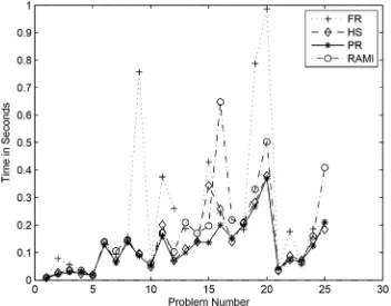
Figure 3. Problem Number Vs Iterations taken by each method to find the weighted analytic center using inexact line search (Quadratic Interpolation) for the 25 problems where all four methods were successful and +=FR, =HS, *=PR, o=RAMI.

(9)

Figure 5. Graph of the Quadratic Approximation P (α) for Problem 30 with w = [4, 6, 5, 3, 106_{, 4] at iteration 12. Note P (α) is flat over the interval [h1, h3] = [0,} 1.9462x10−9_{]. At iteration 13, P (α) does not exist and therefore FR with Quadratic interpolation line search failed.}

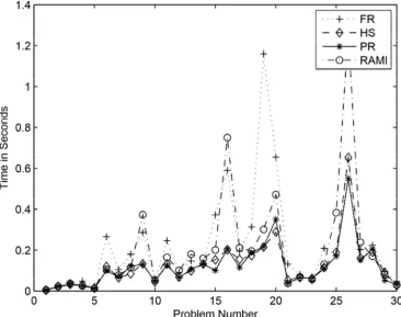
The graph of Problem Number vs. Number of Iterations for Table 3 is given in Figure 1 and Figure 2 is the graph of the Problem Number vs. Time taken. The results in Table 3, Figure 1 and Figure 2 show that PR is the best method in terms of least number of iterations. Table 4 gives the number of iterations and time (in seconds) taken by each method to find the weighted analytic center for the given weights using Quadratic interpolation inexact line search. The entry “⊻_{” means that CG method has failed to find the}

weighted analytic center due to numerical problems and “⊻ ⊻” if it did not converge after the maximum number of 1000 iterations (jamming phenomenon). We see that FR had jamming in three problems, while PR had jamming in one problem and HS in none. This confirms the known fact that FR is more susceptible to jamming than both PR and HS. Figure 3 is the graph of the Problem Number vs. Number of Iterations taken by each method to find the weighted analytic center using inexact line search (Quadratic Interpolation) for the 25 problems where all four methods were successful. The graph of Problem Number vs. Time taken is given in Figure 4. The results in Table 4, Figure 3 and Figure 4 show that PR is the best method in terms of least number of iterations and time, followed by HS, then RAMI, and then FR.

Therefore, FR with Quadratic interpolation line search failed for Problem 30. Our results show that PR and HS are superior to RAMI with the problems considered in this paper, contrary to the results reported in [23].

5. Conclusion

(10)

Acknowledgements

We thank Lieven Vandenberghe of University of California at Los Angeles and Jim Swift of Northern Arizona University for responding to our questions during this research.

References

[1] F. Alizadeh, “Interior Point Methods in Semidefinite Programming with Applications to Combinatorial Optimization”, SIAM Journal on Optimization, vol. 5, no. 1, 1995, pp. 13-51.

[2] L. Vandenberghe and S. Boyd, “Semidefinite Programming”,

SIAM Review, vol. 38, 1996, pp. 49-95.

[3] F. Alizadeh, J. A. Haeberly and M. Overton, “Primal-Dual Methods for Semidefinite Programming: Convergence Rates, Stability and Numerical Results”, SIAM Journal on Optimization, vol. 8, no. 3, 1988, pp. 746-768.

[4] J. Renegar, “A polynomial-time algorithm, based on Newton’s method, for linear programming, ” Math. Programming, vol. 40, 1988, pp. 59–93.

[5] M. J. Todd, K. C. Toh and R. H. Tuntuncu, “On the Nesterov-Todd direction in semidefinite programming,” SIAM J. Optim., vol. 8, 1998, pp. 769-796.

[6] L. Vandenberghe, S.-P. Boyd and S. Wu, “Determinant Maximization with Linear Matrix Inequality Constraints”,

SIAM Journal on Matrix Analysis, vol. 19, no. 2, 1998, pp. 499-533.

[7] I. S. Pressman and S. Jibrin, “A Weighted Analytic Center for Linear Matrix Inequalities”, Journal of Inequalities in Pure and Applied Mathematics, Vol. 2, Issue 3, Article 29, 2002. [8] S. Jibrin and J. W. Swift, “The Boundary of the Weighted

Analytic Center for Linear Matrix inequalities.” Journal of Inequalities in Pure and Applied Mathematics, Vol. 5, Issue 1, Article 14, 2004.

[9] J. Machacek and S. Jibrin, “An Interior Point Method for Solving Semidefinite Programs Using Cutting Planes and Weighted Analytic Centers”, Journal of Applied Mathematics, Vol. 2012, Article ID 946893, 21 pages.

[10] D. S. Atkinson and P. M. Vaidya, “A scaling technique for finding the weighted analytic center of a polytope ” Math. Prog., vol. 57, 1992, pp. 163–192.

[11] S. Jibrin, “Computing Weighted Analytic Center for Linear Matrix Inequalities Using Infeasible Newton’s Method”, Journal of Mathematics, vol. 2015, Article ID 456392, 2015. [12] S. Jibrin, I. Abdullahi, “Search Directions in Infeasible

Newton’s method for Computing Weighted Analytic Center for Linear Matrix Inequalities”, Applied and Computational Mathematics, vol. 8, no. 1, 2019, pp. 21-28.

[13] L. Vandenberghe and S. Boyd, “Convex Optimization”, Cambridge University Press, New York 2004.

[14] W. W. Hager, H. Zhang, “A survey of nonlinear conjugate gradient method”, Pacific Journal of Optimization, vol. 2, no. 1, 2006, pp. 35-58.

[15] M. Rivaie, A. Abashar, M. Mamat and M. Ismail, “The

convergence properties of a new type of conjugate gradient methods”, Applied Mathematical Sciences, vol. 9, no. 54, 2016, pp. 2671-2682.

[16] I. Abdullahi, R. Ahmad, “Convergence Analysis of a New Conjugate Gradient Method for Unconstrained Optimization”,

Applied Mathematical Sciences, vol. 9, no. 140, 2015, pp. 6969-6984.

[17] I. Abdullahi, R. Ahmad, “Global Convergence Analysis of a Nonlinear Conjugate Gradient Method for Unconstrained Optimization Problems”, Indian Journal of Science and Technology, vol. 9, no. 41, DOI: 10.17485/ijst/2016/v9i41/90175, 2016.

[18] I. Abdullahi, R. Ahmad, “Global convergence analysis of a new hybrid conjugate gradient method for unconstrained optimization problems”, Malaysian Journal of Fundamental and Applied Sciences, vol. 2, no. 13, 2017, pp. 40-48.

[19] X. Du, J. Liu, “Global convergence of a spectral hs conjugate gradient method”, Procedia Engineering, vol. 15, 2011, pp. 1487-1492.

[20] W. W. Hager, H. Zhang, “A new conjugate gradient method with guaranteed descent and an efficient line search”, JSIAM Journal on Optimization, vol. 16, no. 1, 2005, pp. 170-192. [21] J. Liu, Y. Feng, “Global convergence of a modified ls nonlinear

conjugate gradient method”, Procedia Engineering, vol. 15, 2011, pp. 4357-4361.

[22] Z. Wei, G. Li, L. Qi, “New nonlinear conjugate gradient formulas for large-scale unconstrained optimization problems”,

Applied Mathematics and Computation, vol. 179, no. 2, 2006, pp. 407-430.

[23] Y. Zhang, H. Zheng, C. Zhang, “Global convergence of a modified PRP conjugate gradient method”, Procedia Engineering, vol. 31, 2012, pp. 986-995.

[24] R. Fletcher, C. M. Reeves, “Function minimization by conjugate gradients”, The computer Journal, vol. 7, no. 2, 1964, pp. 149-154.

[25] B. T. Polyak, “The conjugate gradient method in extremal problems”, USSR Computational Mathematics and Mathematical Physics, vol. 9, no. 4, 1969, pp. 94-112. [26] M. R. Hestenes, E. Stiefel, “Methods of conjugate gradients for

solving linear systems”, Journal of Research of the National Bureau of Standards, vol. 49, 1952, pp. 409-436.

[27] S. Jibrin and I. S. Pressman, “Monte Carlo Algorithms for the Detection of Necessary Linear Matrix Inequalities”,

International Journal of Nonlinear Sciences and Numerical Simulation, vol. 2, no. 2, 2001. pp. 139-154.

[28] R. Burden and D. Faires, “Numerical Analysis”, 9th Ed., Addison Wesley, 2011.

[29] G. Zoutendijk, Nonlinear Programming, Computational Methods, in Integer and Nonlinear Programming, J. Abadie, ed., North-Holland, Amsterdam, 1970, pp. 37-86.

[30] E. Polak and G. Ribiere, “Note sur la convergence de directions conjugees”, Rev. Francaise Informat Recherche Opertionelle, 3e Annee 16, 1969, pp. 35-43.