R E S E A R C H
Open Access
The power-Cauchy negative-binomial:
properties and regression
Muhammad Zubair
1, Muhammad H. Tahir
2, Gauss M. Cordeiro
3*, Ayman Alzaatreh
4and Edwin M. M. Ortega
5*Correspondence: gausscordeiro@gmail.com 3Departamento de Estatística, Universidade Federal de Pernambuco, PE 50740-540, Recife, Brazil
Full list of author information is available at the end of the article
Abstract
We propose and study a new compounded model to extend the half-Cauchy and power-Cauchy distributions, which offers more flexibility in modeling lifetime data. The proposed model is analytically tractable and can be used effectively to analyze
censored and uncensored data sets. Its density function can have various shapes such as reversed-J and right-skewed. It can accommodate different hazard shapes such as decreasing, upside-down bathtub and decreasing-increasing-decreasing. Some mathematical properties of the new distribution can be determined from a linear combination for its density function such as ordinary and incomplete moments. The performance of the maximum likelihood method to estimate the model parameters is investigated by a simulation study. Further, we introduce the new log-power-Cauchy negative-binomial regression model for censored data, which includes as sub-models some widely known regression models that can be applied to censored data. Four real life data sets, of which one is censored, have been analyzed and the new models provide adequate fits.
Keywords: Censoring, Compounding, G-class, Half-Cauchy distribution, Maximum likelihood estimation, Negative-binomial distribution
AMS Subject Classification: Primary 60E05, Secondary 62N05, 62F10
Introduction
Numerous extended classical distributions have been proposed for modelling data in sev-eral areas such as biological studies, environmental and medical sciences, engineering, economics, finance and actuarial science. However, in many applied areas like lifetime analysis, finance and insurance, there is a clear need for further extended distributions, that is, new distributions which are more flexible to model real data in these areas, since the data can present a high degree of skewness and kurtosis. There are many generaliza-tions and extensions of distribugeneraliza-tions in literature using the randomly-stopped approach for either the minimum or maximum ofK independent and identically distributed (iid) random variables (discrete or continuous). See, for example, Nekoukhou and Bidram (2017). Further, Rooks et al. (2010) introduced a two-parameterpower-Cauchy (PC) dis-tribution for analyzing upside-down bathtub (UBT) hazard function data. The cumulative distribution function (cdf ) and probability density function (pdf ) of the PC distribution with shape parameterαand scale parameterσare, respectively, given by
GPC(z;α,σ)=2π−1tan−1(z/σ)α, z>0 α,σ >0 (1)
and
gPC(z;α,σ)=2π−1(α/σ) (z/σ)α−1
1+(z/σ)2α−1. (2) Tahir et al. (2016) studied theexponentiated power-Cauchy (EPC)distribution. LetZa
denote the EPC distribution with baseline parameters α andσ and power parameter a>0. The cdf and pdf ofZaare given by
FEPC(z)=
2π−1tan−1
z
σ
αa
(3)
and
fEPC(z)=2aπ−1
α
σ z σ
α−1
1+z σ
2α −1
2π−1tan−1z σ
αa−1
, (4)
respectively.
In this paper, we define a new four-parameter generalization of the PC distribution named thepower-Cauchy negative-binomial(PCNB) model. The new distribution is flex-ible to model complex positive real data sets, i.e., it can have decreasing, UBT shaped and decreasing-increasing-decreasing hazard rate functions (hrfs). It thus provides a good alternative to several well-known life distributions.
The paper is unfolded as follows. In “The proposed model” section, we define the PCNB distribution. In “Properties of the new model” section, we obtain some of its mathematical properties including quantile function (qf ), tail behaviors, a useful linear representation for its density function and some types of moments. In “Estimation” section, the model parameters are estimated by maximum likelihood and a simulation study is performed. In “Regression model” section, we present a regression model based on the PCNB distribu-tion with censored data. In “Applicadistribu-tions” secdistribu-tion, the usefulness of the new distribudistribu-tion is illustrated by means of four real data sets where we show empirically that it out-performs some well-known lifetime distributions. Finally, “Concluding remarks” section offers some concluding remarks.
The proposed model
General Insurance companies typically face two major problems when they want to use past or present claim amounts in forecasting future claim severity. First, they have to find an appropriate statistical distribution for their large volumes of claim amounts. Then, test how well this statistical distribution fits their claim data. Most data in general insurance problems is skewed to the right and therefore most distributions that exhibit this charac-teristic can be used to model the claim severity. Insurance data contains relatively large claim amounts, which may be infrequent. Hence, there is a clear need to use statistical distributions with relatively heavy tails and highly skewed like the PC distribution.
LetT1,. . .,TK denote the failure times ofK(a latent random variable) claims whereK
is assumed independent of theTis in a set-up with at least one claim. Then, we defineZ= max{T1,. . .,TK}. Consider that theTis are iid random variables with common cdfG(z)
and thatKfollows the negative-binomial (NB) probability mass function (n=1, 2,. . .and pare fixed but unknown parameters)
P(K=k)=
k−1 n−1
pn(1−p)k−n,k=n,n+1,. . ., p∈(0, 1).
Under this set-up, the conditional pdf ofZgivenKis
f(z|K =k)=k g(z)G(z)k−1.
Then, the marginal pdf ofZfollows as
f(z) = ∞
k=n
k g(z)G(z)k−1
k−1 n−1
pn(1−p)k−n
= ( png(z)
1−p)nG(z)
∞
k=n
k
k−1
n−1 (1−p)G(z)
k
= n png(z)G(z)n−1
1−(1−p)G(z)n+1. (5) The cdf ofZ(which holds for any positive realn) is given by
F(z) =
pG(z) 1−(1−p)G(z)
n
. (6)
Inserting Eqs. (1) and (2) in Eq. (5), we obtain
f(z)= 2π
−1n pn(α/σ) (z/σ)α−11+(z/σ)2α−1
2π−1tan−1(z/σ)αn−1
1−2π−1(1−p) tan−1(z/σ)αn+1 , (7)
whereα,σ >0 andp∈(0, 1). Henceforth, we denote byZ∼PCNB(n,p,α,σ)a random variable having the density (7). The cdf ofZis given by
F(z)=F(z;n,p,α,σ)=
2π−1ptan−1(z/σ)α 1−2π−1(1−p)tan−1(z/σ)α
n
. (8)
Clearly, ifp=n=1, the PCNB model is identical to the PC distribution (2). Moreover, the PCNB(n,p,α,σ)model has the following six sub-models:
(i) Ifp=n=α=1, it gives the half-Cauchy (HC) distribution;
(ii) Ifα=1, it reduces to the half-Cauchy negative binomial (HCNB) distribution; (iii) Ifn=1, it gives the PC-geometric distribution;
(iv) Ifα=n=1, it becomes the HC-geometric distribution; (v) Ifp=1, it reduces to the exponentiated-PC distribution; (vi) Ifp=n=1, it becomes the PC distribution.
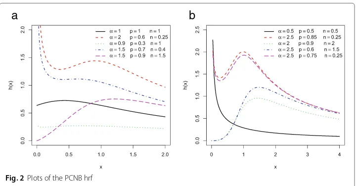
a
b
Fig. 1Plots of the PCNB density
and b indicate that the hrf ofZ can have DFR (decreasing failure rate), UBT and DID (decreasing-increasing-decreasing) shapes.
Properties of the new model
In this section, we provide some structural properties of the new distribution.
Quantile function and random number generation The qf ofZis determined by inverting (8) as
Q(u)=σ
tan
π
u1/n 2 [p+(1−p)u1/n]
1/α
, u∈(0, 1). (9)
We can easily generate PCNB random variables from (9).
a
b
Tail behaviors
The tail behaviors of the pdf and cdf ofZin (7) and (8) are given as follow:
f(z)∼nαA znα−1, as z→0+,
f(z)∼αB z−α−1, as z→ ∞,
F(z)∼A znα, as z→0+,
1−F(z)∼B z−α, as z→ ∞,
whereA = (2p/π)n andB = 2n/(pπ). For example, for fixed values ofnandp, the left and right tails of the PCNB distribution are heavier whenαincreases. Also, for fixed values ofαandp, the left tail becomes heavier whennincreases.
Moments
For any real q > 0, the power series (1−t)−q = ∞j=0(q)jtj/j! holds, where(q)j =
q+(q+1)+· · ·+(q+j−1)=(q+j)/ (q)is the ascending order factorial and(q)0=1.
Then, the cdf ofZin Eq. (8) can be expressed as
F(z) = ∞
j=0
Bj(n,p)GPC(z;α,σ)n+j, (10)
whereBj(n,p)=(n)jpn(1−p)j/j! (forj≥0) andGPC(z;α,σ)is the cdf given in Eq. (1).
By differentiating Eq. (10), the pdf ofZfollows as
f(z) = ∞
j=0
Bj(n,p)hn+j(z), (11)
wherehn+j(z) = hn+j(z;α,σ)is the EPC density function with power parametern+j
given by Eq. (4). Equation (11) reveals that the PCNB density is a linear combination of EPC densities. So, some mathematical properties ofZcan be obtained from those of the EPC distribution. Next, we provide two examples.
Tahir et al. (2016) (see Sections 6.8 and 6.9) determined thesth ordinary and incomplete moments ofZaas
EZas=aσs ∞
i=0
(0.5π)2i+αs ai(s/α)
(a+2i +s/α) (12)
and
z 0
zsfEPC(z)dz=aσs
∞
i=0
(0.5π)2i+s/αai(s/α)Daz+2i+s/α
a+2i +s/α , (13)
respectively, where a0(s) = 1, a1(s) = s/3, a2(s) = s(5s + 7)/90, etc, and Dz =
2π−1tan−1(z/σ)α.
Then, therth ordinary moment ofZfollows from Eqs. (11) and (12) as
μ
r=E(Zr)=
∞
i,j=0
Bj(n,p)(
n+j) σr (0.5π)2i+r/α a i(r/α)
n+j + 2i+ r/α . (14)
Analogously, therth incomplete moment ofZ, say mr(z) =
z
0zrfPCNB(z)dz, can be
obtained from (11) and (13) as
mr(z)=σr
∞
i,j=0
Bj(n,p)ai(r/α)(
n+j) (0.5π)2i+r/αDzn+j+2i+r/α
The first incomplete momentm1(q)follows from Eq. (15) forr=1. It is useful to obtain
the Bonferroni and Lorenz curves and mean deviations for the new model.
Estimation
Several approaches for parameter point estimation were proposed in the literature but the maximum likelihood method is the most commonly employed. The maximum likelihood estimates (MLEs) enjoy desirable properties that can be used when constructing confi-dence intervals for the model parameters. Large sample theory for these estimates delivers simple approximations that work well in finite samples. The normal approximation for the MLEs in distribution theory is easily handled either analytically or numerically.
We consider the estimation of the unknown parameters of the new distribution by the maximum likelihood method. Letz1,. . .,zm bemobserved values from the PCNB
dis-tribution given by (7) with vector of parameters θ = (n,p,α,σ). The log-likelihood =(θ)forθis given by
= mlog2n pnπ−1(α/σ)+(α−1)
m
i=1
log(zi/σ)− m
i=1
log1+(zi/σ)2α
+(n−1)
m
i=1
log[(2/π)tan−1(zi/σ)α]
−(n+1)
m
i=1
log1−(1−p)[(2/π)tan−1(zi/σ)α]
. (16)
Equation (16) can be maximized either directly by using well-known computing platforms such as theR(optimfunction),SAS(PROC NLMIXED) andOxprogram (sub-routineMaxBFGS). These scripts can be applied and executed for a wide range of initial values. This process often leads to more than one maximum. However, in these cases, we consider the MLEs corresponding to the largest value of the log-likelihood statistics. In a few cases, no maximum is identified for the selected initial values. In these cases, new initial values can be tried in order to obtain a maximum. There exist sufficient conditions for the existence of the MLEs such as compactness of the parameter space and the con-cavity of the log-likelihood function. These estimates can exist even when such conditions are not satisfied. For more complex models, and in particular when there is no explicit solution, it is nearly impossible to establish theoretical conditions on the existence and uniqueness of the MLEs. However, such properties can be investigated numerically for this distribution and a given data set.
For interval estimation on the model parameters, we can evaluate the estimated observed information matrixJ(θ) numerically. Further, we can easily check if the fit using the PCNB model is statistically “superior” to the fits using any of its six special models. For example, for comparing the PCNB and HC distributions, i.e., testing the null hypoth-esisH0 : p = n = α = 1 againstH1 : H0is false, the likelihood ratio (LR) statistic is
given byw=2{(θ)−(θ)}, whereθandθ are the unrestricted and restricted estimates obtained by maximizing= (θ)underH1andH0, respectively. The limiting
distribu-tion of this statistic isχ32under the null hypothesis, which is rejected ifwexceeds the upper 100(1−γ )% quantile of theχ32distribution.
a situation, where the time to event is not completely observed and is subjected to right censoring. LetCidenote censoring time. We then observezi =min(ti,ci), wheretiis the
observed time to the event andciis the observed right-censored, fori = 1,. . .,m. The
log-likelihood function reduces to
(θ) = ci m
i=1
log2npnπ−1(α/σ)+(α−1)log(zi/σ) −log1+(zi/σ)2α
−(m−1)log2π−1tan−1(zi/σ)α
−(m+1)log1−2(1−p)π−1tan−1(zi/σ)α
+(1−ci) m
i=1
log
1−
2pπ−1tan−1(zi/σ)α
1−2(1−p)π−1tan−1(z i/σ)α
.
The above log-likelihood can be maximized numerically to obtain the MLEs. We use theoptimroutine in theRsoftware.
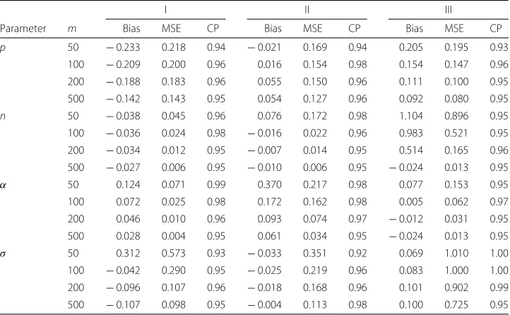
Monte Carlo simulation study.Now we assess the performance of the maximum like-lihood method for estimating the PCNB parameters using Monte Carlo simulations. The simulation study is repeated 5000 times each with sample sizesm=50, 100, 200, 500 and parameter scenarios: I:p=0.8,n=0.5,α =0.5 andσ =1, II:p=0.5,n=0.5,α=1.5 andσ =1 and III:p=0.1,n=1.5,α=1.5 andσ =1. Table 1 gives the average biases (Bias) of the MLEs, mean square errors (MSE) and model-based coverage probabilities (CP) for the parametersp,n,αandσ under these scenarios and different sample sizes. Based on the simulation results, we conclude that the MLEs perform well in estimating the parameters of the PCNB distribution. The CPs of the confidence intervals are quite close to the 95% nominal levels. Therefore, the MLEs and their asymptotic results can be adopted for estimating and constructing confidence intervals for the model parameters.
Table 1Monte Carlo simulation results: Biases, MSEs and CPs
I II III
Parameter m Bias MSE CP Bias MSE CP Bias MSE CP
Regression model
In many practical applications, the lifetimes are affected by explanatory variables such as the cholesterol level, blood pressure, weight and many others. Parametric models to esti-mate univariate survival functions and for censored data regression problems are widely used. A regression model that provides a good fit to lifetime data tends to yield more precise estimates of the quantities of interest.
In applications in the area of survival analysis, the hrf is often U-shaped or unimodal, i.e., the function is not monotonic. The regression models commonly used for survival data are the log-Weibull, monotonic failure rate, log-logistic, decreasing failure rate and unimodal functions. One of the objectives of this work is to propose a new regres-sion model, in location and scale form, called thelog-power-Cauchy negative-binomial (LPCNB) regression model, which presents different failure rate functional forms. The proposed model is an alternative to the traditional extreme value (or log-Weibull), logistic and log-normal models, among others. One way to study the effect of these explanatory variables on the response variableY is through a location-scale regression model, also known as a model of accelerated lifetime. These models consider that the response vari-able belongs to a family of distributions characterized by a location parameter and a scale parameter. Further details on this class of regression models can be found in Cox and Oakes (1984), Kalbfleisch and Prentice (2002) and Lawless (2003). In the context of sur-vival analysis, some distributions have been used to analyze censored data. For example, more recently, Cruz et al. (2016) proposed the log-odd log-logistic Weibull regression model with censored data, Lanjoni et al. (2016) defined an extended Burr XII regres-sion model and Ortega et al. (2016) introduced the odd Birnbaum-Saunders regresregres-sion model with applications to lifetime data. In a similar manner, we define a location-scale regression model using the LPCNB regression model.
LetZ∼PCNB(n,p,α,σ)be a random variable having the density (7). A class of regres-sion models for location and scale is characterized by the fact that the random variable Y =log(Z)has a distribution with location parameterμ(v), which depends only on the explanatory variable vector, and a scale parametera. Then, we can writeY=μ(v)+aW, wherea>0 and the distribution ofWdoes not depend onv.
The random variableY =log(X)re-parameterized in terms ofμ=log(σ)anda=α−1 has density function (fory∈R) given by
f(y) =
2p π
n nexp
y−μ a
arctan(n−1)
exp
y−μ a
a1−(1−p)2π−1arctanexpy−μ a
(n+1), (17)
wheren> 0 andp∈ (0, 1)are shape parameters,μ ∈ Ris the location parameter and a>0 is the scale parameter.
We refer to Eq. (17) as the LPCNB distribution, sayY ∼ LPCNB(n,p,μ,a). IfZ ∼ PCNB(n,p,α,σ), thenY=log(Z)∼LPCNB(n,p,μ,a).
Forp = n = 1, we obtain the log-power Cauchy (LPC) model. The survival function corresponding to Eq. (17) is given by
S(y)=1−
2p π
n arctann
exp
y−μ a
1−(1−p)2π−1arctanexpy−μ a
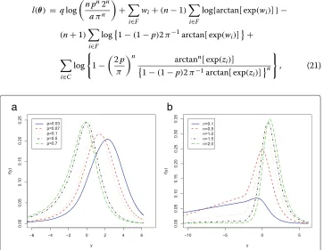
Plots of the density function (17) for selected parameter values are displayed in Fig. 3a and b, which show great flexibility for different values ofpandn.
We define the standardized random variable W = (Y − μ)/a having the density function
f(w)=
2p π
n nexp(w)arctanexp(w)(n−1)
1−(1−p)2π−1arctanexp(w)(n+1). (19)
Next, we propose a linear location-scale regression model linking the response variable yiand the explanatory variable vectorvTi =(vi1,. . .,vip)given by
yi=vTi τ+a wi, i=1,. . .,m, (20)
where the random errorwihas density function (19),τ =(τ1,. . .,τp)T,a>0,n>0 and
p ∈ (0, 1)are unknown parameters. The parameterφi = vTi τ is the location ofyi. The
location parameter vectorφ = (φ1,. . .,φm)T is represented by a linear modelφ = vτ,
whereV = (v1,. . .,vm)T is a known model matrix. The LPCNB model (20) opens new
possibilities for fitting many different types of data.
Consider a sample(y1,v1),. . .,(ym,vm) ofm independent observations, where each
random response is defined byyi = min{log(zi), log(ci)}. We assume non-informative
censoring such that the observed lifetimes and censoring times are independent. Let F and C be the sets of individuals for which yi is the log-lifetime or log-censoring,
respectively. Conventional likelihood estimation techniques can be applied here. The log-likelihood function for the vector of parametersθ = p,n,a,τTT from model (20) has
the forml(θ) =
i∈F
li(θ)+ i∈C
l(ic)(θ), whereli(θ) = log[f(yi)],l(ic)(θ) =log[S(yi)],f(yi)
is the density (17) andS(yi) is the survival function (18) ofYi. The total log-likelihood
function forθ reduces to
l(θ) = qlog
n pn2n aπn
+
i∈F
wi+(n−1)
i∈F
log{arctan[ exp(wi)]} −
(n+1)
i∈F
log1−(1−p)2π−1arctan[ exp(wi)]
+
i∈C
log
1−
2p π
n arctann[ exp(z i)]
1−(1−p)2π−1arctan[ exp(z i)]
n
, (21)
a
b
whereqis the number of uncensored observations (failures) andwi=
yi−vTi τ
/a. The MLEθofθcan be evaluated by maximizing the log-likelihood (21). We use the procedure NLMixed in SAS to calculateθ. Initial values forτ andaare taken from the fit of the LPC regression model withp=n=1.
The elements of the (p+ 3) × (p+ 3) observed information matrix J(θ), namely Jpp,Jpn,Jpa,Jpτj,Jnn,Jna,Jnτj,Jaa,Jaτj andJτjτs (forj,s =1,. . .,p), can be evaluated numer-ically. Inference onθ can be conducted in the classical way based on the approximate multivariate normalNp+3
0,J(θ)−1distribution forθ.
We can use the likelihood ratio (LR) statistic for comparing some special models with
the LPCNB regression model. We consider the partitionθ =
θT 1,θT2
T
, where θ1is
a subset of parameters of interest andθ2is a subset of remaining parameters. The LR
statistic for testing the null hypothesisH0 : θ1 = θ(10) versus the alternative
hypothe-sis H1 : θ1 = θ1(0) is given byw = 2{(θ)−(θ)} , whereθ andθ are the estimates
under the null and alternative hypotheses, respectively. The statisticwis asymptotically (asn→ ∞) distributed asχq2, whereqis the dimension of the subset of parametersθ1
of interest.
Applications
In this section, the PCNB distribution is fitted to model three real life data sets. We compare the fits of the PCNB model with the beta-Weibull (BW) proposed by Lee et al. (2007), beta half-Cauchy (BHC) defined by Cordeiro and Lemonte (2011), Kumaraswamy half-Cauchy (KHC) presented by Ghosh (2014), power-Cauchy geometric (PCG) and power-Cauchy models. We estimate the parameters by using the maximum likelihood method. In order to compare the models, we consider the following goodness-of-fit statis-tics: Akaike information criterion (AIC) and Kolmogorov-Smirnov (K-S) measure with the associatedp-value. The pdfs of the BW, BHC and KHC (forx>0 anda,b,c,σ,λ >0) distributions are given by
fBW(x) =
c λB(a,b)
x
λ
c−1
e−b(λx)c1−e−(xλ)ca−1, fBHC(x) = K1
1+x σ
2 −1
tan−1x σ
a−1
1−2π−1tan−1x σ
b−1
,
fKHC(x) = K2
1+x σ
2 −1
tan−1x σ
a−1
1−2π−1tan−1x σ
ab−1
,
respectively, whereK1=2a/[σ πaB(a,b)] andK2=a b2a/(σ πa).
Table 2MLEs, their SEs (in parentheses) and goodness-of-fit measures for the first data set
Distribution Estimates AIC K-S p-value
PCNB(α,p,n,σ) 1.8529 0.0029 0.3905 3.5171 487.1582 0.0791 0.9131 (0.3737) (0.0015) (0.1375) (1.6477)
BW(a, b, c,λ) 8.9783 0.10422 0.5264 0.3086 489.5797 0.1028 0.6655 (3.9535) (0.0224) (0.0250) (0.0033)
PCG(α,p,σ) 1.182 71.1917 0.9153 492.4754 0.0911 0.8009 (0.1415) (6.7322) (0.9334)
BHC(a,b,σ) 1.5514 0.9514 11.1816 499.1124 0.1256 0.4096 (0.6308) (0.3152) (9.3295)
KHC(a,b,σ) 1.3321 0.9188 14.3689 497.3825 0.1528 0.1936 (0.8090) (0.3935) (7.9620)
PC(α,σ) 1.0127 25.1088 492.7543 0.0877 0.8360 (0.1271) (5.2807)
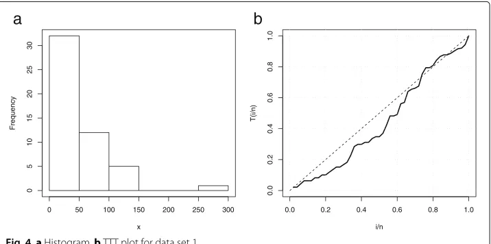
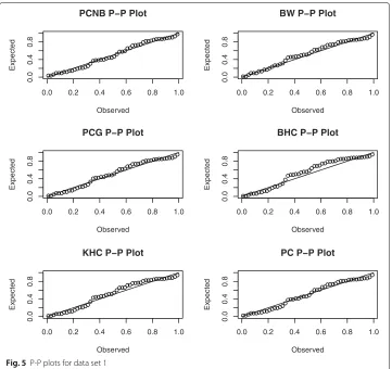
these data in Fig. 4b. The summary statistics and Fig. 4a and b reveal that the first data set is skewed with DID failure rate shape. So, the PCNB has the ability to fit right-skewed data with DID failure rate shape. For a visual comparison, we provide PP plots of the fitted models to these data in Fig. 5. Clearly, the PCNB model provides a closer fit to these data.
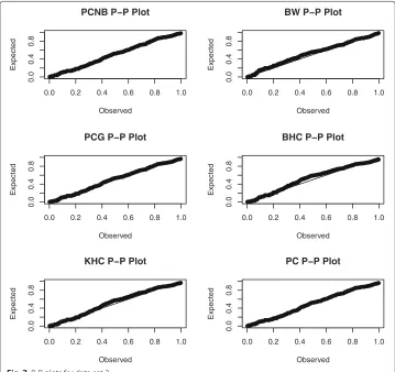
Data set 2: Jet Airplanes failure data. The second data set is taken from Porchan (1963), which represents the failure times of air conditioning system of 720 jet airplanes. A set of the summary statistics of the data are:m=213,x= 93.14085,¯ s=106.7636, skew-ness=2.11185 and kurtosis=4.92499. The results of the fitted distributions are presented in Table 3. We conclude that the PCNB model provides the best fit with lowest values of the AIC and K-S statistics and largestp-value. The scaled TTT plot for the second data set in Fig. 6b gives an indication of a decreasing failure rate shape. The summary statistics and Fig. 6a and b reveal that the second data set is right-skewed with decreasing failure shape. So, the PCNB distribution can be used effectively to model these data. The PP plots in Fig. 7 also support the results of Table 3.
In conclusion, the PCNB model is certainly an appropriate model for fitting the first two data sets.
a
b
Fig. 5P-P plots for data set 1
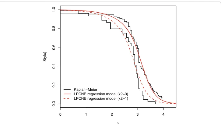
Data set 3: Head and neck cancer data. The third data set is taken from Efron (1988) regarding head and neck cancer clinical trial consisting of survival times of 51 patients inarm Awho were given radiation therapy. Nine patients were lost to the follow-up and were regarded as censored observations. The MLEs of the model parameters are listed in Table 4. The figures in this table indicate that the PCNB model provides the best fit with
Table 3MLEs, their SEs (in parentheses) and goodness-of-fit measures for the second data set
Distribution Estimates AIC K-S p-value
PCNB(α,p,n,σ) 1.6228 0.0035 0.7221 2.8888 2364.093 0.046 0.7588 (0.1972) (0.0009) (0.1969) (1.7041)
BW(a, b, c,λ) 7.6164 0.1194 0.568 1.1134 2367.086 0.0767 0.1632 (1.5171) (0.0088) 0.0025) (0.0033)
PCG(α,p,σ) 1.3668 76.7098 2.9658 2368.893 0.0483 0.6507 (0.0905) (131.7613) (3.3747)
BHC(a,b,σ) 1.7824 0.9400 22.1049 2388.513 0.1029 0.0219 (0.2498) (0.1014) (4.6448)
KHC(a,b,σa) 1.4395 1.1559 36.2886 2375.904 0.0837 0.1013 (0.1744) (0.1462) (7.4700)
PC(α,σ) 1.1812 53.1034 2369.847 0.0524 0.6033
a
b
Fig. 6aHistogram,bTTT plot for data set 2
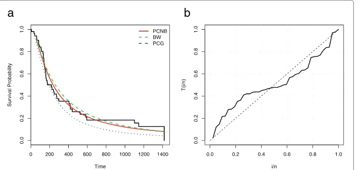
lowest values of the AIC and K-S statistics. The plot in Fig. 8b reveals that the third data set has UBT failure rate shape, and then the PCNB distribution can be used effectively to model these data. The plots of the estimated survival functions of the PCNB, BW and GPC distributions are displayed in Fig. 8a. Clearly, the PCNB estimated survival function provides a closer fit to the empirical survival function than the other models.
Table 4MLEs, their SEs (in parentheses) and goodness-of-fit measures for the third data set
Distribution Estimates AIC BIC
PCNB(α,p,n,σ) 1.2865 0.0070 1.6620 4.2398 592.1857 599.9130 (0.2690) (0.0055) (1.0335) (6.2151)
BW(a, b, c,λ) 17.8517 0.7694 0.3143 4.0437 594.1023 601.8296 (59.5446) (1.8538) (0.4824) (25.6600)
PCG(α,p,σ) 1.4738 0.0053 9.2046 599.0166 604.8121 (0.1888) (0.0041) (6.0303)
BHC(a,b,σ) 1.9480 1.0755 127.2517 598.7476 604.5431 (0.6174) (0.2655) (54.0490)
KHC(a,b,σ) 1.9059 1.0921 130.6862 598.7297 604.5252 (0.6031) (0.2780) (55.0280)
PC(α,σ) 0.5788 45.3099 649.3128 653.1764
(0.1101) (12.3464)
Regression model example : Entomology data. First, we use the data from a study car-ried out at the Department of Entomology of the Luiz de Queiroz School of Agriculture, University of São Paulo, which aims to assess the longevity of the Mediterranean fruit fly (ceratitis capitata). The need for this fly to seek food just after emerging from the lar-val stage has permitted the use of toxic baits for its management in Brazilian orchards for at least fifty years. This pest control technique consists of using small portions of food laced with an insecticide, generally an organophosphate, that quickly kills the flies, instead of using an insecticide alone. Recently, there have been reports of the insecticidal effect of extracts of the neem tree leading to proposals to adopt various extracts (aqueous extract of the seeds, methanol extract of the leaves and dichloromethane extract of the branches) to control pests such as the Mediterranean fruit fly. The experiment was com-pletely randomized with eleven treatments, consisting of different extracts of the neem tree, at concentrations of 39, 225 and 888 ppm.
After preliminary statistical analysis, these eleven treatments were allocated into two groups, namely:
a
b
Table 5MLEs of the parameters from the LPCNB regression model fitted to the entomology data
set, the corresponding SEs (given in parentheses),p-values in [·]
Model a n p τ0 τ1 τ2
LPCNB 0.2514 0.4118 0.1496 2.9793 0.0188 -0.2787
(0.0383) (0.0897) (0.1470) (0.1471) (0.0779) (0.0854) [<0.001] [0.8098] [0.0013]
LPC 0.4100 1 1 3.0781 -0.0207 -0.2779
(0.0293) (0.0617) (0.0832) (0.0939)
[<0.001] [0.8038] [0.0035]
• Group 1: Control 1 (deionized water); Control 2 (acetone - 5%); aqueous extract of seeds (AES) (39 ppm); AES (225 ppm); AES (888 ppm); methanol extract of leaves (MEL) (225 ppm); MEL (888 ppm); and dichloromethane extract of branches (DMB) (39 ppm).
• Group 2: MEL (39 ppm); DMB (225ppm) and DMB (888 ppm).
The response variable in the experiment is the lifetime of the adult flies in days after exposure to the treatments. The experimental period was set at 51 days, so that the num-bers of larvae that survived beyond this period were considered as censored data. The total sample size isn=72, because four observations were lost. Therefore, the variables used in this study are:zi-lifetime of ceratitis capitata adults in days,vi1-sex of the larvae
andvi2-group (0=group 1, 1=group 2). We start the analysis of these data considering only
failure (zi) and censoring (ci) data and an appropriate model for fitting the data could be
the LPCNB and LPC distributions.
Next, we present results on fitting the model
yi=τ0+τ1vi1+τ2vi2+awi,
where the response variableYifollows the LPCNB distribution given in (17),i=1,. . ., 72.
Table 5 lists the MLEs and their standard errors in parentheses for two fitted regression models. The MLEs of the model parameters are evaluated using the NLMixed procedure in SAS. Iterative maximization of the logarithm of the likelihood function (21) starts with initial values forτandσ, which are taken from the fit of the LPC regression model.
We note from the fitted LPCNB regression model thatv2is significant at 1% and that
there is a significant difference between the groups 1 and 2 for the survival times. Table 6 gives a summary of the AIC, consistent Akaike information criterion (CAIC) and Bayesian information criterion (BIC) to compare the LPCNB and LPC regression models. The LPCNB regression model outperforms the LPC model irrespective of the criteria and then they can be used effectively in the analysis of these data.
Finally, we turn to a simplified model retaining onlyv2as an explanatory variable
yi=τ0+τ2vi2+a wi.
Table 6AIC, CAIC and BIC statistics for comparing the LPCNB and LPC regression models
Model AIC CAIC BIC
LPCNB 332.8 333.4 351.7
Table 7MLEs of the parameters from the fitted LPCNB regression model to the entomology data
Model a n p τ0 τ2
LPCNB 0.2532 0.4164 0.1569 2.9917 -0.2771
(0.0375) (0.0879) (0.1496) (0.1391) (0.0846) [<0.001] [0.0013]
The MLEs for the LPCNB regression model fitted to these data are listed in Table 7. In order to assess if the model is appropriate, Fig. 9 displays the plots of the empirical survival function and the estimated survival function from the fitted LPCNB regression model. In fact, this regression model provides a good fit to these data.
Concluding remarks
We consider a lifetime model in the context of insurance claims where the claim sizes follow a power Cauchy and the number of claims is negative binomial distributed. In these terms, we propose a new model by compounding the power-Cauchy and negative-binomial distributions called thepower-Cauchy negative-binomial(PCNB) distribution. We provide a useful linear representation for its density, which allows to obtain some properties for the proposed distribution. We use the maximum likelihood method for estimating the model parameters. The suitability of these estimates is investigated by a simulation study. We fit the proposed distribution to three real data sets to show empir-ically its flexibility. We proposed a new class of regression models for location and scale based on the logarithm of the PCNB random variable. Estimation and inference on the regression coefficients are discussed and an application to real data in Entomology is addressed. Various future studies can be conducted, such as employing other estima-tion techniques (bootstrap and Bayesian methods) and investigating the sensitivity of the LPCNB regression model using diagnosis and analysis of residuals. which led to this improved version.
Acknowledgement
The authors are grateful to the Editor-in-Chief, the Associate Editor and anonymous referees for their many helpful comments and suggestions on an earlier version of this paper which led to this improved version.
Authors’ contributions
The authors, viz MZ, MHT, GMC, AA and EMMO with the consultation of each other carried out this work and drafted the manuscript together. All authors read and approved the final manuscript.
Competing interests
The authors declare that they have no competing interests.
Publisher’s Note
Springer Nature remains neutral with regard to jurisdictional claims in published maps and institutional affiliations.
Author details
1Department of Statistics, Govt. S.E. College, Bahawalpur, Pakistan, 63100 Bahawalpur, Pakistan.2Department of Statistics, The Islamia University of Bahawalpur, 63100 Bahawalpur, Pakistan.3Departamento de Estatística, Universidade Federal de Pernambuco, PE 50740-540, Recife, Brazil.4Department of Mathematics and Statistics, American University of Sharjah, 26666 Sharjah, UAE.5Departamento de Ciências Exatas, ESALQ, Universidade de São Paulo, Piracicaba/SP, Brazil.
Received: 24 January 2017 Accepted: 11 December 2017
References
Aarset, MV: How to identify bathtub hazard rate. IEEE Trans. Reliab.36, 106–108 (1987)
Cordeiro, GM, Lemonte, AJ: The beta-half Cauchy distribution. J. Probab. Statist. Art. ID. (904705), 18 (2011) Cox, DR, Oakes, D: Analysis of survival data. Chapman and Hall, New York (1984)
Cruz, da, Ortega, JN, Cordeiro, EMM: GM: The log-odd log-logistic Weibull regression model: modelling, estimation, influence diagnostics and residual analysis. J. Stat. Comput. Simul.86, 1516–1538 (2016)
Efron, B: Logistic regression, survival analysis, and the Kaplan–Meier curve. J. Amer. Statist. Assoc.83, 414–425 (1988) Ghosh, I: The Kumaraswamy-half Cauchy distribution: Properties and applications. J. Stat. Theory Appl.13, 122–134 (2014) Kalbfleisch, JD, Prentice, RL: The statistical analysis of failure time data. Wiley, New York (2002)
Kumar, U, Klefsjo, B, Granholm, S: Reliability investigation for a fleet of load haul dump machines in a Swedish mine. Reliab. Eng. Syst. Safet.26, 341–361 (1989)
Lanjoni, BR, Ortega, EMM, Cordeiro, GM: Extended Burr XII regression models: Theory and applications. J. Agric. Biol. Environ. Stat.21, 203–224 (2016)
Lawless, JF: Statistical models and methods for lifetime data. Wiley, New Jersey (2003)
Lee, C, Famoye, F, Olumolade, O: Beta-Weibull distribution: Some properties and applications to censored data. J. Mod. Appl. Stat. Methods.6, 173–186 (2007)
Nekoukhou, V, Bidram, H: A new generalization of the Weibull-geometric distribution with bathtub failure rate. Commun. Stat. Theory Methods.46, 4296–4310 (2017)
Ortega, EMM, Lemonte, AJ, Cordeiro, GM, da Cruz, JN: The odd Birnbaum-Saunders regression model with applications to lifetime data. J. Stat. Theory Pract.10, 780–804 (2016)
Proschan, F: Theoretical explanation of observed decreasing failure rate. Technometrics.5, 375–383 (1963) Rooks, B, Schumacher, A, Cooray, K: The power Cauchy distribution: derivation, description, and composite models.
NSF-REU Program Reports (2010). Available from "http://www.cst.cmich.edu/mathematics/research/REU_and_LURE. shtml"
![Table 5 MLEs of the parameters from the LPCNB regression model fitted to the entomology dataset, the corresponding SEs (given in parentheses), p-values in [·]](https://thumb-us.123doks.com/thumbv2/123dok_us/949564.1593867/15.595.118.479.110.201/table-parameters-lpcnb-regression-entomology-dataset-corresponding-parentheses.webp)