Volume 2008, Article ID 824195,14pages doi:10.1155/2008/824195
Research Article
A Color Topographic Map Based on the Dichromatic
Reflectance Model
Mich `ele Gouiff `es and Bertrand Zavidovique
Institut d’Electronique Fondamentale, CNRS UMR 8622, Universit´e Paris-Sud 11, 91405 ORSAY Cedex, France
Correspondence should be addressed to Mich`ele Gouiff`es,michele.gouiff[email protected]
Received 19 July 2007; Accepted 21 January 2008
Recommended by Konstantinos Plataniotis
Topographic maps are an interesting alternative to edge-based techniques common in computer vision applications. Indeed, unlike edges, level lines are closed and less sensitive to external parameters. They provide a compact geometrical representation of images and they are, to some extent, robust to contrast changes. The aim of this paper is to propose a novel and vectorial representation of color topographic maps. In contrast with existing color topographic maps, it does not require any color conversion. For this purpose, our technique refers to the dichromatic reflectance model, which explains the distribution of colors as the mixture of two reflectance components, related either to the body or to the specular reflection. Thus, instead of defining the topographic map along the sole luminance direction in theRGBspace, we propose to designcolor linesalong each dominant color vector, from the body reflection. Experimental results show that this approach provides a better tradeoffbetween the compactness and the quality of a topographic map.
Copyright © 2008 M. Gouiff`es and B. Zavidovique. This is an open access article distributed under the Creative Commons Attribution License, which permits unrestricted use, distribution, and reproduction in any medium, provided the original work is properly cited.
1. INTRODUCTION
According to the morphology concepts [1], the most relevant information of an image is provided by the level sets, independently of their actual level. The topographic map [2] embeds the boundaries of the level sets, that is, it is defined as the collection of level lines. Their computation is quite simple, since they can be obtained by a multithresholding procedure. However, they are said to be more stable than edges which suffer from incompleteness and sensitivity to external parameters, for example, threshold to extract them after some gradient computation. The level lines never cross but superimpose and completely structure the image. More-over, this representation is invariant against uniform contrast changes. These properties explain the interest in computer vision applications: extraction of meaningful lines to pro-duce a more compact representation of the image [3–5], robust image registration and matching correspondences [6,7], segmentation through variational approaches [8,9], where level sets provide a good initialization for the iterative process. Moreover, robust features, such as junctions and
segments of level lines, have been used successfully in match-ing processes, for instance in the context of stereovision for obstacle detection [10].
The challenging problem addressed in this paper is the definition of a color extension to gray-level lines. Due to the increased volume of data by a factor of three, expected benefits are an improved robustness of the application, that is usually the case with multispectral fusion in general, and a significant compression for the same information. The computer vision procedure has to be robust to illumination changes, especially to contrast changes, else than respective to some class of visual context (e.g., given contrast changes) then through experiments. Information would better relate to some tasks to be completed in a satisfactory manner. Indeed, using color in the context of segmentation or matching can largely reduce ambiguities while improving the quality of results.
each color component in a marginal manner. This would produce some redundant results and artifacts, and bring a puzzling question up: fusing lines from different color bands while maintaining the inclusion property. The authors use the HSV color space, the components of which are less correlated thanRGB’s. Also, this representation is claimed to be in adequacy with perception rules of the human visual system. However, they favor the intensity for the definition of the topographic map. Unfortunately, since the hue is ill-defined with unsaturated colors, this kind of a representation may output irrelevant level sets due to the noise produced by the color conversion at a low saturation. A sensible and trivial solution should be to use a modified HSV space able to take the color relevancy into account, as done for instance in [13] for the definition of a color gradient.
In order to avoid this kind of issue, we define a novel concept of color lines by considering the physical process of interaction between light and matter, which explains the color perception. Indeed, the spectrum of the radiance reaching the sensor depends jointly on the light spectrum and on the material features. This phenomenon can be described in theRGB space by the dichromatic reflectance model [14]. Notwithstanding its simplicity, this model has proved to be relevant for many kinds of materials and it is widely used in computer vision [15–20].
In this formalism, any color of a uniform inhomoge-neous and Lambertian object is located roughly along a straight line linking the origin of theRGBspace (black) to the intrinsic color of the material. Motivated by such modeling, the proposed color topographic map is a multidirectional extension of the unidirectional gray-level lines, since the color sets and lines are defined along every diffuse color in a polar fashion. Thus, it is additionally adaptive to the image content, since the directions of the diffuse colors are computed. Last but not least, this new representation does not require any nonlinear color conversion, therefore reducing the subsequent artifacts. The main expected benefit is a reduction of the amount of level lines while preserving the image structure so that the complexity of the appli-cation concerned, for example matching or tracking, be lowered.
This article is organized as follows. Section 2 recalls the definition and main properties of gray-level lines and details the principles of the existing color topographic maps. Then,Section 3details the image formation model on which the proposed method is based: the dichromatic reflectance model. The novel color topographic map is the subject of
Section 4. We first explain its main principles, and second we focus on its technical implementation. Its invariance to color changes is also discussed. To conclude, Section 5
asserts the relevance of the proposed method by comparing our topographic map with results from preiously existing techniques.
2. TOPOGRAPHIC REPRESENTATION OF
THE IMAGE
The topographic map was introduced in [2]. This section recalls its definition and its main properties.
2.1. Gray topographic map
Definition 1. LetI(p) be the image intensity at pixelp.Ican be decomposed into upper level sets
Nu(E)=p,I(p)≥E (1)
or lower level sets
Nl(E)=p,I(p)≤E. (2)
The parameterE expresses the considered level. The topo-graphic map is obtained by computing the level sets for each
E in the gray-level range:E ∈[0,. . ., 2nb−1], for an image coded onnbdigits.
Property 1. Equations (1) and (2) yield the inclusion prop-erty of level sets:
Nu(E+dE)⊂Nu(E), Nl(E)⊂Nl(E+dE),
whereE+dE ≥E.
(3)
Property 2. Both images of upper level setsINuor lower level
setsINl contain all information needed to reconstruct the
initial image I by using the occlusionO and transparency
Toperations :
I(p)=OINu(p)=supE,p∈NuE (4)
or
I(p)=TINl(p)
=infE,p∈Nl
E
. (5)
Definition 2. Boundaries of level sets are called level lines
LE and form a set of Jordan curves. This set provides a comprehensive description of the image. Indeed, the latter can be reconstructed from it, unlike from edges. The set of the level lines is called the topographic map and forms an inclusion tree.
Property 3. Because of the inclusion property of level sets (Property 1), level lines do never overlay or cross.
Despite the good properties of gray-level lines, few works have been carried out to propose their extension to multispectral images. To our knowledge, only two methods have been proposed, they are detailed hereafter.
2.2. Color topographic map
The main difficulty to obtain an adequate description of color lines (i.e., showing the same properties as level lines: completeness, inclusion, and contrast invariance) is to deal with the three-dimensional nature of color. The gray scale is naturally, totally, and well ordered, whereas the 3D color cube is not easily ordered in a way that fits the rules of color perception.
Colored topographic map
RGB and better fitting the human perception. First, they compute the topographic maps of luminance and for each connected component they consider it as piecewise constant, the color of which is given by the mean saturation and hue. They show that the geometric structure of a color image is contained in its gray-level topographic map and the geometric information provided by color, far from contradicting the gray-level geometry, is complementary. As a conclusion, the color lines are similar to the gray-level lines, but the colors of the sets can be quite different from the original image content.
Total order in the HSV space
However, two different colors can have the same intensity values, therefore some information is lost by considering gray levels only. The method proposed by [12] is to our mind more appropriate to color handling since the three components of HSV are considered. The authors define a total lexicographic order of colors on R3 by favoring intensity first, then hue and saturation, in order to imitate the perception rules of the human visual system. LetU1 = (L1,H1,S1) andU2 = (L2,H2,S2) be two colors; the order betweenU1andU2is given by
U1U2 if
L1L2
orL1=L2
andH1< H2
or L1=L2
andH1=H2
andS1< S2
.
(6)
Although it follows the human visual system, this specific order does not take into account specificities of the HSV space, namely, the fact that hue is ill-defined for low saturation. Defining directly color sets in the RGBspace is one of the solutions to address that question.
In the next section, we detail the reflectance model used to define our color topographic map.
3. THE DICHROMATIC REFLECTANCE MODEL
The dichromatic reflectance model proposed by Shafer [14] is based on the Kubelka-Munk theory. It states that any inhomogeneous dielectric material, uniformly colored and dull, reflects light either by interface reflection or by body reflection. In the first case, the reflected beam preserves more or less the spectral characteristics of the incident light, thus the color stimulus is generally assumed to be the same as the illuminant color. The body reflection results from the penetration of the light beams in the material, and from its scattering by the pigments of the object. It depends on the wavelength λ and on the physical characteristics of the considered material. Theoretically, the dichromatic reflectance model is only valid for the scenes which are lighted by a single illuminant without any interreflections. Despite these limitations, it has proved to be appropriate for many materials and many acquisition configurations.
LetPbe a point of the scene andpits projection into the image. In general, the object radianceL(λ,P) can be seen as
the sum of two radiative terms, the body reflectionLb(λ,P) and the surface radianceLs(λ,P):
L(λ,P)=Lb(λ,P) +Ls(λ,P). (7)
Each of the termsLbandLscan be decomposed, such that
L(λ,P)=I(λ,P)Rb(λ,P)mb(P) +I(λ,P)ms(P), (8)
where mb and ms are two functions which depend only on the scene geometry, whereasRb(λ,P) andI(λ,P) refer, respectively, to the diffuse radiance and illuminant spectrum. By integration of the stimulus on the tri-CCD camera, of sensitivities Si(λ) (i = R,G,B), it leads to the color component of the diffuse reflection cb(p) =
cR
b,cbG,cBb
T
and the color vector of the specular reflection cs(p) =
cR s,cGs,cBs
T
at pixelp:
ci
b(p)=Ki
λSi(λ)
I(λ,P)Rb(λ,P)dλ,
ci
s(λ,p)=Ki
λSi(λ)
I(λ,P)dλ.
(9)
The termKiexpresses the gain of the camera in the sensori. Thus, the dichromatic model inRGBspace becomes
c(p)=mb(p)cb(p) +ms(p)cs(p). (10)
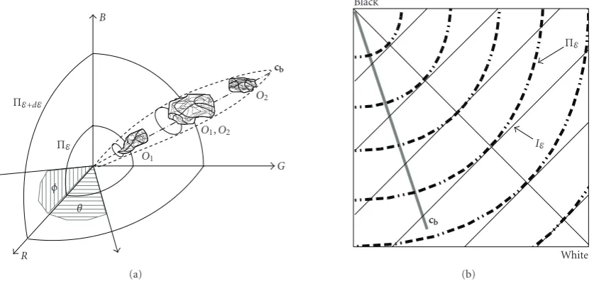
According to (10), the colors of a material are distributed in theRGBspace on a planar surface defined bycs(p) and
cb(p) as it is sketched inFigure 1(a). However, according to [21–23], the colors of a specular material are located more precisely in an L-shape cluster; the vertical bar of the L
goes from the origin RGB =(0, 0, 0)T to the diffuse color componentcb, and the horizontal bar of theLgoes fromcbto the illuminant colorcs. That case is illustrated inFigure 1(b). For faintly saturated images, colors are distributed roughly along the intensity direction.
In the remaining of the article, the objects are assumed to be Lambertian, so that the illuminant contribution is neglected and the termms(p)cs(p) vanishes in (10).
Remark 1. In other words, an approximation is made here: in changing the location of the illuminant color in theRGB
R
B
G
c
cs
cb
(a)
R
B
G
c
cs
cb
(b)
Figure1: (a) General dichromatic model. The colors of a homogeneous material are located on a plane defined bycbandcs. (b) TheL-shape
dichromatic model. This sketch corresponds to the specular case withmb=ms=1/2.
Blu
e
Gre en
Red
c1b c2
b
Caps (a)
Blu
e
Re d
c1b c2b
c3b c4
b
Baboon (b)
Figure2: Examples of color images with their color distribution in theRGBspace (ColorSpace Software, available onhttp://www.couleur .org/). Body vectors are perfectly visible in the case of little textured images of “Caps.” The vectors are less distinguishable on the image of “Baboon.”
4. A COLOR TOPOGRAPHIC MAP IN ACCORDANCE
WITH THE DICHROMATIC MODEL
One of our motivations is to extract color sets and lines in accordance with the image content without any color conversion. As underlined in the previous section, the colors of most natural images are roughly located along a finite number of straight lines in the RGB space, that is along each body reflection vectorcb. Our idea is to split the color space up along these lines, around which the meaningful information is contained. Consequently, our problem is to lose the least possible of the meaningful information conveyed by the image while scanning the RGB space in accordance with this information in a polar fashion. Unlike existing color sets [11, 12] (seeSection 2.2), the proposed technique does not require any color conversion and does not favor the intensity as in [11].
The first subsection hereafter explains the main princi-ples of the color set extraction, which involves two steps, while the second subsection details more accurately the technical steps of the algorithm.
4.1. Principles
While gray-level sets are extracted along the luminance axis of theRGBspace, our color sets are extracted along each body reflection vectorcbrevealed by the image.
In that context, we can consider a spherical frame in the
RGB space, each color being located by its distance to the origin (the black color) and its zenithal and azimuthal angles. The first step of the algorithm captures colors according to their distance from the black without distinguishing between directions cb. Second, and that is one of the originalities of the proposed method, the sets are defined independently along each color dominant vector.
4.1.1. Stage 1: extraction of color setsN(E)
R
B
G
ΠE+dE
ΠE
φ
θ
O1
O1,O2 O2
cb
(a)
Black
White
ΠE
IE
cb
(b)
Figure3: (a) Two isosurfaces in theRGBspace. (b) Comparison between the isodistance sphere and its corresponding intensity plane.
line, treating the distance is sufficient. Favoring the distance levels instead of the luminance ones allows to treat every direction of theRGBspace without any preference.
We choose to quantize this distance uniformly. Let us considerKcolor sets at a distanceE∈ {Emin. . .Emax}. These color sets consist of points such that their color distance to the black is greater thanE (for upper color sets).
Definition 3 (isosurface ΠE). One calls ΠE the spherical
isosurface which is the locus of any color appearing at a distanceEfrom the black. As an example,Figure 3(a)shows two isosurfaces,ΠEandΠE+dE, in theRGBspace.
Definition 4(color setN(E)). Colorsccan be layered into upper level sets in the following way:
Nu(E)= p,c(p)≥E (11)
and the lower color sets are defined as
Nl(E)= p,c(p)≤E (12)
on the luminance axis, whereR=G=B=I, that is strictly equivalent to gray-level sets computed along the luminance axis as in [2, 12]. For a given distance E, the surfaces ΠE
intersect each and every body vector color with regular and identical stepsE in the wholeRGBspace (seeFigure 3(b)) which sketches a section along the luminance axis). On the other hand, the corresponding intensity planes, called IE, intersect these vectors with varying stepsE≥E. Moreover, sinceE ≥ E, the upper gray-level sets are included in the corresponding color sets.
Theoretically, theRGBcomponents of the pixels belong-ing to a color setN(E) are located along the straight linecb, either above the spherical isosurfaceΠEfor upper color sets
or underΠEfor lower color sets.
Obviously, an upper color setNu(E +dE) is included in the upper level set Nu(E). Let us underline again that the first interlevel sets contain the shading and dark pixels. In opposition, the last ones are likely to contain specular reflection and white objects.
Remark 2. The distance used here to define the color sets is the Euclidean distance, but one could use distances related to the sensitivity of the human visual system, such as the CIELAB distance. Unfortunately, it would require the conversion in the CIELAB space which needs some a priori information about the illuminant color.
Definition 5 (connected component CCE). One calls CCi
E
the ith connected component of the color setN(E) for a given region 2D-ordering in the picture.
Remark 3. At this stage, a given object (orCCE) can consist of several dominant colors in theRGBspace and, conversely, the same body color can appear as several regions (objects) in the image. In that respect,Figure 3(a)is likely representing the colors of two real objectsO1andO2, the colors of which are mixed on the same body vector.
Figure 4 illustrates the extraction of the CCE on the image “House” (see Figure 4(a)). The upper color set (for
E = 60) produces two connected components, drawn in white inFigure 1(b).
In addition to the physical interpretation, rather than psychological, central to our approach, the prime difference at that stage between [12] and ours is to (partially) order the color cube in a polar fashion rather than Cartesian.
4.1.2. Stage 2: extraction of color subsetsM
C2
C1
C2
(a)
CC1 E
CC2 E
(b)
CS1 E
CS2 E
CS3 E
(c)
Figure4: Color sets and subsets extraction in the image “House.” (a) Initial image. (b) Extraction of the first color set (E =60). The white pixels are the pixels belonging to the upper color set. (c) After spherical projection and clustering, the connected componentCCE2is replaced
by two connected components of different colorsCS2
EandCS3E.
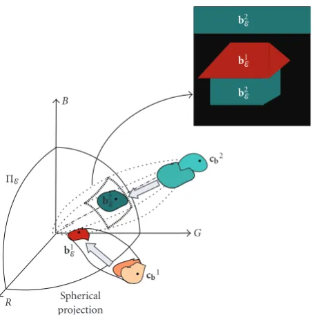
b2
E
b1E
b2E
R
G B
b1E b2
E
cb1
cb2
ΠE
Spherical projection
Figure5: Projection of two body vectors onto the isosurfaceΠE.
The body colorcbiprojects inbiE ontoΠE. In the image, pixels are
clustered to the nearest color.
number of body colors. In that case, the color sets defined in stage 1 cannot be distinguished from one another, therefore the angular information (zenithal and azimuthal angles) is required.Figure 5illustrates this situation for two dominant vectors of theRGBspace.
First of all, let us assume that the body colors cbi are known. We will explain a computation key in Section 4.2. Let us focus on upper color sets, where all the colors ofCCE
are located above the spherical isosurfaceΠE. We callc(p) a
color present inCCEandcE(p) its spherical projection onto
the isosurfaceΠE. In the same way, we callbiEthe projection
of the body colorcbi. Since the dichromatic model assumes
that the colorsc(p) of a body are all located around a vector cb, then all the spherical projectionscE(p) are located around
bi
E onto the surfaceΠE. InFigure 5, the projections onΠE
form two density modes, drawn in red and turquoise in this example.
Thus, we consider each connected componentCCEof the color setN(E) and divide it into as many color subsetsMas there are body colors.
Definition 6(color subsetM(bi
E)). The color subsetM(biE)
is the set of all pixels the color of which clusters aroundbi
E:
M(biE)= p,cE(p)−biE<cE(p)−bjE, ∀j /=i
.
(13)
Each pixel gets the color value of the projected body colorbj
E from which it is the closest. Therefore, each color
set N(E) consists of different subsets of colors bj
E, the
corresponding pixels of which are segmented into connected components of the image.
Definition 7(connected componentCSE). One callsCSEithe
ith connected component of the color subsetM(bE) for the
same image region-ordering as inDefinition 3.
Figure 4(c)illustrates the color subsetsCSE obtained on the image “House,” for two body colors. We note that a single color setCCcan be divided into several color subsetsCSE.
Figure 5shows more precisely the projection from the
RGB space to the image “House.” Here, two subsets of colorsb1
E andb2E are extracted, after the colors have been
projected ontoΠE.
At the next step of the algorithm, the color sets of level
E +dE are computed on each and every color subsetCSE
previously obtained. Stages 1 and 2 are repeated as necessary. The procedure stops when the level is equal toEmax.
Definition 8 (color lines). The color lines are defined as the boundaries of the connected components extracted in
M(bi
Eventually, benefits of the inclusion property inherent to gray-level lines need to be secured. No order is explicitly required between colors since the order is obtained directly in the image by inclusion of the connected components. So far, we did not explain the procedure to compute body colors. To that aim, the next subsection details the steps involved in the extraction of the topographic map.
4.2. Implementation
This subsection describes successively the technique chosen to exhibit the body colors and the underlying data structure.
4.2.1. Computation of the body colors
Once the color setsN(E) have been extracted, the connected componentsCCE can consist of several objects of different body colors cb. Since the number of colors is unknown, the separation problem translates into a nonsupervised clustering problem. According to the dichromatic model, colors are roughly clustered around a straight line linking the black to the unknown body color. Among that cluster, we assume that the most likely body color vector is the line of maximum color density. Similarly, it is assumed that by projecting these colors spherically onto ΠE, the
intersection ofcbwithΠEwill be the locus where the density
of projections is maximum.
Thus, for each connected componentCCE extracted in the color setN(E) (seeDefinition 2), we consider all color vectorsc(p) located in the upper color set and compute their projectioncE(p)=(RE,GE,BE)Tonto the isosurfaceΠE:
RE(p)= R·E
c, GE(p)=
G·E
c, BE(p)=
B·E
c. (14)
By considering the angles described inFigure 3(a), we carry out the transformation from Cartesian coordinates cE to
spherical ones (ρ,θ,φ):
ρ=cE,
θ=arctan
GE RE
, if RE=/ 0, θ=π
2 otherwise,
φ=arctan
BE REcosθ
, ifREcosθ /=0, φ=π
2 otherwise. (15)
In this 2D space defined by the zenithal and azimuthal angles in the RGBspace (θ,φ), we compute the histogram
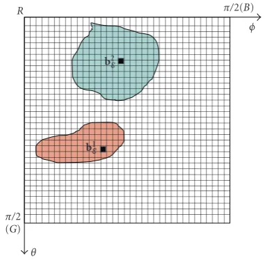
HE(θ,φ) of the color projections originating from the connected componentCCE.Figure 6shows an example of histogramHE(θ,φ) for two body colors. Let us underline that possible values of angles (θ,φ) can be quantized in order to efficiently reduce the amount of data.
Eventually, the number of body colors stems from the number of connected components in the 2D histogram
HE(θ,φ) (seeFigure 6). On each connected component, the
R
π/2 (G)
π/2(B)
b1 E
b2 E
φ
θ
Figure6: HistogramHE(θ,φ) of the projections of colors onto the
spherical planeΠE.
body colorbiEis assigned the bin (θ,φ) for whichHE(θ,φ) is maximum.
Once the body colors bEi have been extracted, each
connected component CCE of the color set N(E) is seg-mented to produce the color subsetsM(bEi) of colorbEi. The
connected componentsCS are obtained through a region-growing procedure by using the homogeneity criterion given in (13). This mechanism is sketched inFigure 5: two color vectors form two projection modes on the surface ΠE.
The colors bE1 and bE2 are computed, and the image is
segmented.
Remark 4. Either the same quantization ofHE(θ,φ) is used for the whole levelsE or it can be adaptive to it, for instance to maintain the same numberNbinsof bins whatever the value ofE. Indeed, the size of the isosurface depends directly on its location in theRGBspace (seeFigure 3(a)). It is maximum whenE=2nb−1 if the image is coded onnbbits and the width of a bin in the histogram for a given value ofE isS= (π/2)(E/Nbins).
4.2.2. The data structures
The description of the image in terms of color sets is achieved in a general tree structure that can be fruitfully exploited in the image segmentation and for further image matching. Let us refer toFigure 7to illustrate the states of the tree during the first extraction of color sets and color subsets on the image “House.” The father node is the level set associated to
Emin, but generallyEmin = 0 so that this node contains the entire image. The sons of the top node are the connected components CCE extracted in the father color set. Then, after computation of the color subsets, a component CCE
can be replaced by several connected componentsCS (see
Father Father Father
CCE1 CCE2 CS1E CS2E CS3E CS1E CS2E CS3E
CS2
E+dE CS3E+dE
(a) (b) (c)
Figure7: Color sets and subsets extraction in the tree structure computed from the image “House” (Figure 4). (a) State of the tree after computation of the first upper color sets. (b) State of the tree after computation of the first color subsets. The nodeCC2 is
replaced by two color subsetsCS2andCS3. (c) State of the tree after
the extraction of the second color sets.
At each subsequent stage of the algorithm, the sons at levelE become the fathers of some new color sets at level
E+dE. Each node is thus attributed a distance valueEand a color value.
A stack is used to register nodes to be treated. After all sons of a node have been computed, this node will not be visited anymore. The sons are put in the stack to be treated later and a new current node at color distance E is pulled out of the stack. On the connected component associated to the current node, we first compute the color setN(E+dE) and the color subsetsM(bi
E), as previously explained. The
algorithm stops when the stack is empty.
The flowchart of the algorithm is sketched inFigure 8. After the color sets extraction, the level lines are defined as the boundaries of color sets. The following subsection discusses the invariance of the topographic map towards color changes.
4.3. Influence of color changes on the topographic map
Spherical scale changes.Let I1 andI2 be two color images, whereI2is obtained fromI1by spherical scale changeT. If we consider a colorc1ofI1andc2the corresponding one in I2, they are related by the transformc2=Tc1for allc1in the
RGBspace with
T=c2
c1. (16)
By considering this transformation, it influences the length of the straight lines without changing their directions. This color change is sketched inFigure 9(b). For the sake of clarity, the color vectors are represented on a dichromatic plane (C1,C2) = {(R,G), (B,R), (G,B)}. The topographic maps of I2 and I1 are similar when their associated number of color levels is the same. Therefore, the topographic map is invariant to spherical scale change when E2 = E1/T, where E2 and E1 are the color levels used to compute the topographic maps of I2 and I1, respectively. When colors are not saturated, the transformT amounts to the classical intensity contrast changeT=I2/I1, withI1andI2being two intensity values.
Angular changes
Since the topographic map is defined along straight lines from the black to dominant colors, they are invariant to angular rotations of these vectors with center black. This change is sketched in Figure 9(c). As noticed in (9) and subsequent remark, this type of color change would result either from a shift of the spectrum of the illuminantI(λ,P) or from a change in the camera sensitivitySi(see conclusion of Section 3). Section 5 will show some validation results which compare the robustness of the topographic maps to illumination changes.
5. VALIDATION
We now compare our representation of color sets with the topographic maps described, respectively, in [11] (on value V) and [12] (by a total order in the HSV space).
Let us define the a priori best collection of level sets as the one which can reconstruct the image at best with the lowest number of level sets. Therefore, we consider the conjunction of the following criteria:
(i) the number of setsNsetsof the topographic map, which refers to the reduction of the amount of data;
(ii) the dissimilarity between the collection of level sets extracted and the initial image, to be measured via the mean CIELAB distance DCIE76. It corresponds to the Euclidean distance computed in the CIELAB space, relating to a real perceptual difference (see, e.g., [24]). We assume an illuminantd65, being most common since it represents the average daylight. Some other distances, such as the S-CIELAB [25], are more efficient but they require some additional knowledge about the observation distance, which is unknown and variable. The classical PSNR will be also used later in the paper for quantitative results.
In addition, we will compare the execution times of the three techniques and the robustness of the topographic maps (in terms of lines location) to illuminant changes.
Qualitative comparison.
First of all, let us introduce the five representative images shown inFigure 2(“Caps” and “Baboon”) and inFigure 10
(“Synthetic,” “Statue,” and “Girl”) that we focus on here. The image of “Caps” represents an ideal example where objects are quite uniform, with almost no texture. “Synthetic” is an artificial image with color scales. “Statue” (this image is extracted from the Kodak image database) is almost unsaturated. “Girl” and “Baboon” show some texture and color shadings.
Our topographic map is compared to the results obtained by the two methods described inSection 2.2. To distinguish between them, we use the following notation:
RGB image
E=Emin Threshold E
Colour set
Connected components
analysis
CC1 E
CCNE
Computation of body colours
Computation of body colours
Segmen-tation
Segmen-tation
CS1 E
CSM E
E=E+dE E
· · · . .
. ... ... ...
Stack
Figure8: Flowchart of the computation of the color topographic map. The image is thresholded with the current parameterEto obtain the color setN. Then,Nconnected components are extracted. On each of them the body colors are computed by histogram analysis, and the image is segmented to obtainMcolor subsets. They are put in the stack to be treated, with an increased parameterE =E+dE.A new subset of levelEis pulled out of the stack to be processed, and the color sets are extracted from it. The algorithm stops when the stack is empty.
C1
C2 c
1
E1
(a)
C1 C2
c1
c2
E2
(b)
C1 C2
c1
c2
(c)
Figure9: Invariance to color illuminant changes. (a) Example of two body vectors in the color plane (R,G). (b) Scale changeT:c2=Tc1.
(c) Rotation change.
In order to compare the topographic maps exhibited by different techniques, it is necessary to choose identical parameters. Thus, we consider 10 levels on hue and satura-tion for technique B. Similarly, we use a constant bin size 10 ×10 for the histogramHE(θ,φ) computed in the proposed method C (see Section 4.2.1). Five quantization levels Nl (from 8 up to 64 levels) are tested either on luminance for methods A and B or on the distance to black for method C.
Let us refer toTable 1, which collects the values ofNsets and DCIE76 for the three methods (columns) and the five images (rows) and for the different quantization levels.
Naturally, the number of sets is always lower for A than for B. Indeed, in both cases, the color sets are established in the HSV space, but A designs them by using luminance information only, while B scans the whole HSV space. For the same reason, theDCIE76 is always greater for A than for
B. Thus, B provides a less compact structure of the image but preserves better the color information.
By considering now the averages of the criteria (itemμ
inTable 1), our technique C produces the lowest number of sets in most cases, even compared to the technique A that is carried out on luminance. Nevertheless, theDCIE76 result is not affected by this reduction of data and is even better in most cases. Thus, for the different images considered, our topographic map provides a good compactness of data while preserving correctly the color information.
Synthetic (a)
Statue (b)
Girl (c) Figure10: Images used in the validation experiments.
(a) (b) (c)
(d) (e) (f)
Figure11: Color sets (first row) and lines (second row) obtained on the image “Synthetic” for 16 levels.
InFigure 11, we can see that the method A loses some level lines related to shadings, for instance on the green oval. Similarly, the blue circle is not segmented correctly. Results obtained by techniques B and C are globally satisfying, but C yields 587 lines against 1318 for B, yet including a few defects. The light part of the blue rectangle is better rendered with C than with B. That is true also for the purple rectangle.
Table1: Comparison of the level sets for several numbers of levelsNl, for 5 images and 3 methods (A: [11], B: [12], C: proposed method).
The comparison criteria are the number of setsNsetsand the meanDCIE76computed on the whole image.μrefers to the mean criteria,
computed on the 5Nl.
A [11] B [12] C (our method)
Nl Nsets DCIE76 Nl Nsets DCIE76 Nl Nsets DCIE76
64 879 10,67 64 1318 7,73 64 587 3,22
32 581 10,80 32 976 10,68 32 438 3,34
16 527 14,16 16 901 8,77 16 337 7,65
8 346 24,71 8 719 10,23 8 208 8,29
4 132 36,96 4 543 17,36 4 50 11,78
μ 397 19,46 μ 785 10,95 μ 324 6,86
Synthetic (356×238)
Nl Nsets DCIE76 Nl Nsets DCIE76 Nl Nsets DCIE76
64 8165 2,78 64 17481 3,21 64 7855 2,10
32 3443 6,03 32 12589 6,56 32 3138 5,22
16 2270 14,34 16 11141 15,42 16 1996 12,86
8 1189 28,02 8 9243 30,23 8 983 22,28
4 371 37,65 4 7566 52,42 4 142 32,01
μ 3088 17,76 μ 11604 21,57 μ 3496 14,89
Statue (200×150)
Nl Nsets DCIE76 Nl Nsets DCIE76 Nl Nsets DCIE76
64 6709 4,19 64 12558 2,37 64 5209 1,02
32 2999 11,57 32 9329 4,89 32 2273 2,15
16 2071 15,21 16 8189 7,61 16 1567 4,23
8 1233 22,44 8 7081 11,37 8 889 6,38
4 401 34,67 4 5820 15,46 4 176 15,67
μ 3253 17,62 μ 8595 8,34 μ 2023 5,89
Girl (356×236)
Nl Nsets DCIE76 Nl Nsets DCIE76 Nl Nsets DCIE76
64 6751 9,02 64 11591 9,10 64 5919 3,03
32 3424 9,52 32 9785 9,38 32 2958 3,41
16 2349 11,66 16 8941 10,30 16 1878 5,01
8 1221 15,72 8 7896 12,92 8 964 6,99
4 442 31,55 4 6352 21,53 4 273 12,84
μ 2837 15,49 μ 8913 12,65 μ 2389 6,26
Baboon (356×356)
Nl Nsets DCIE76 Nl Nsets DCIE76 Nl Nsets DCIE76
64 8001 3,04 64 4805 3,25 64 3900 1,26
32 5469 4,25 32 2382 5,77 32 2109 2,23
16 4770 8,72 16 1763 7,23 16 1352 4,37
8 3864 16,41 8 926 10,74 8 759 6,23
4 3116 19,16 4 257 14,18 4 225 7,64
μ 5044 10,23 μ 2027 8,23 μ 1669 4,35
Caps (356×238)
B and C seem qualitatively comparable, however 2273 lines have been produced by C against 9329 by B, that is about four times less lines.
Quantitative results.
We have tested both methods B and C as the two most relevant ones on 210 images from the kodak database
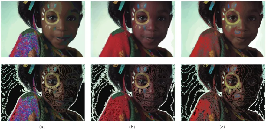
(a) (b) (c) Figure12: Color sets (first row) and lines (second row) obtained on the image “Girl” for 64 levels.
Table 2: Quantitative results obtained on 210 images (Kodak, Arborgreens, Australia, Cambridge bases) for (a) 8 levels and (b) 32 levels. Our color sets based on the dichromatic model (method C) are compared to the color sets designed in the HSV space [12] (method B) by considering the number of sets and the similarity simultaneously (μ: average,σ: SD).
Method Number of sets DCIE76
μ σ μ σ
(a) 8 levels
B 4563,85 1972,41 16,63 5,5
C 436,91 211,6 7,74 4,22
(b) 32 levels
B 7107,76 2892,11 4,02 0,88
C 3719,5 1691,64 2,67 0,84
and gardens. Table 2 collects the results obtained in terms of the number of sets and the mean dissimilarity (DCIE76), respectively, for 8 and 32 levels.μandσ refer to the average and SD of the criteria.
Note that, whatever the quantization level, C exhibits a smaller number of sets while preserving better the color information (lower distance), what asserts the previous analysis. Indeed, for 8 levels (Figure 2(a)), C produces 10 times less sets than B, whereas the mean color distance is 2 times inferior. For 32 levels (Figure 2(b)), C yields only 2 times less sets but the color distance is almost twice lower than for B.
Thus, some conclusions emerge from the previous experiments . First of all, the proposed topographic map is compact: it provides a strong reduction of data while preserving the color information. This is due to the definition of the color sets along the dominant color vectors of the RGB space. Nevertheless, for very textured images, a coarse quantization cannot render all details correctly.
On the other hand, methods defined in the HSV space provide a large number of sets, which is partly due to the production of irrelevant sets for low saturation. Eventually, let us make the comparison more complete in analyzing the robustness of the topographic maps to illumination changes and comparing execution times.
Robustness to illumination changes.
The robustness of the topographic maps is analyzed here by considering the lines locations under different illuminants. First, let us assume that the “Girl” image (Figure 10) has been acquired under the illuminant d65 (average daylight) throughout the visible spectrum. Then, different changes of illuminant have been simulated using the software ColorSpace (this software is freely available on the website:
http://www.couleur.org/). Eight illuminants have been used:
b, e, d50, d55, d75, d95, f10, and f11. For a comparison criterion, in each method we consider the percentage of line points which keeps the same location as in the initial image acquired under the illuminant d65. These values are reported in Figure 13. They show that the method C provides a topographic map which is more stable than both techniques A and B, since a larger number of points are preserved from an illuminant to the other. Indeed, it is well known that the HSV space is not robust to changes of the illuminant spectrum but only to intensity changes (see, e.g., [15]). Topographic maps based on the dichromatic model are confirmed quasi-invariant to some more comprehensive illumination changes than mere intensity variations, as described inSection 4.3.
Execution times.
Table 3: Execution times (in seconds) for different numbers of levelsNl, and for the methods A, B, and C.
Nl A [11] B [12] C (our method)
64 5,11 15,70 19,02
32 1,88 5,32 13,59
16 0,75 3,55 6,51
8 0,25 2,57 3,18
4 0,19 1,41 2,36
f11 f10 d95 d75 d55 d50 e b
0.775 0.75 0.725 0.7 0.675 0.65 0.625 0.6 0.575 0.55 0.525 0.5
Proposed method A
B
Figure13: Evaluation of the robustness of topographic maps to illuminant changes. The curves indicate the percentage of points of the topographic map which remains at the same locations as in the initial image under illuminantd65.
“Girl” (Figure 10), by averaging the times of ten executions of the algorithms. No specific algorithmic optimization has been carried out and the computer used has one processor Intel(R) T2300 1.66 GHz with a 1Go RAM memory. One can notice that method A is far less time-consuming than the two other methods, since the topographic map is computed only on the luminance axis. Our method C is the slowest. That is mainly due to the additional estimation of the body colors, by projection of the colors onto the isosphere and clustering. However, being a mere coordinate transformation (matrix product), the projection could be reduced to anO(1) time on most architectures.
6. CONCLUSION
The topographic map is a compact and complete rep-resentation of an image, which is theoretically robust to global contrast changes. In this article, we have designed a novel color topographic map led by the color dichromatic model. The latter explains the shape of the color distribution in the RGB space. This modeling is initially intended for inhomogeneous and dull material, but the literature has often underlined its relevance for various kinds of materials and for several computer vision applications. It states that
colors of a Lambertian object roughly cluster around some diffuse straight line in theRGBspace.
Unlike existing representations, the proposed map does not require any color conversion, for instance in a perceptual space. Therefore, it overcomes the main defect of these repre-sentations which is the definition of hue for low saturation. The scan of theRGB space depends directly on the image content, that is on the directions of dominant colors. First of all, colors are ordered according to their distance to the black and color sets are defined subsequently. Second, these color sets are split up in color subsets depending on the number of dominant colors located in the color set. Therefore, the level sets are defined along the above-mentioned diffuse vectors. Thus, the proposed topographic map is a multidirectional extension of the gray-level sets which are defined along the luminance axis inRGBspace. The inclusion property of the sets is secured by a combination of spatial connectivity and color partial ordering.
The experimental results have compared the compact-ness and quality of our topographic maps with those obtained by two existing methods, computed in the HSV space. They have shown that the proposed method yields a good tradeoff, since the number of sets obtained is lower while better preserving the structure of the image. The data reduction towards a few robust features is likely to reduce the complexity of the downstream algorithms, as matching or tracking.
Moreover, this technique is robust first to some color changes occurring when the illuminant spectrum varies and second to contrast changes expressed by spherical scale changes of the RGB space. Unfortunately, these improve-ments are done at the cost of a stronger algorithmic com-plexity.
Since the results obtained are encouraging a priori, our future work will focus on implementing the color lines for stereo matching and tracking, based on segments and junctions. The expected result is an improved robustness, by matching the most relevant features while ignoring color illuminant changes. We will also experiment the algorithm by privileging first the directions of the colors instead of favoring distance to black first. Better results with textured images should result from an astute tradeoffto profit from the evolution of the local maxima along the color lines, as well as from better characterizing the histogram-clusters.
REFERENCES
[1] J. Serra,Image Analysis and Mathematical Morphology, Aca-demic Press, Orlando, Fla, USA, 1983.
[2] V. Caselles, B. Coll, and J.-M. Morel, “Topographic maps and local contrast changes in natural images,”International Journal of Computer Vision, vol. 33, no. 1, pp. 5–27, 1999.
[3] A. Desolneux, L. Moisan, and J-M. Morel, “Edge detection by helmhotz principle,”Journal of Mathematical Imaging and Vision, vol. 14, no. 3, pp. 271–284, 2001.
[5] J. Froment, “Perceptible level lines and isoperimetric ratio,” in Proceedings of the International Conference on Image Processing (ICIP ’00), vol. 2, pp. 112–115, Vancouver, BC, Canada, Sep-tember 2000.
[6] P. Monasse and F. Guichard, “Fast computation of a contrast-invariant image representation,”IEEE Transactions on Image Processing, vol. 9, no. 5, pp. 860–872, 2000.
[7] S. Bouchafa and B. Zavidovique, “Efficient cumulative match-ing for image registration,” Image and Vision Computing, vol. 24, no. 1, pp. 70–79, 2006.
[8] C. Kervrann and A. Trubuil, “Optimal level curves and global minimizers of cost functionals in image segmentation,” Journal of Mathematical Imaging and Vision, vol. 17, no. 2, pp. 153–174, 2002.
[9] C. Ballester, V. Caselles, L. Igual, and L. Garrido, “Level lines selection with variational models for segmentation and encoding,”Journal of Mathematical Imaging and Vision, vol. 27, no. 1, pp. 5–27, 2007.
[10] N. Suvonvorn and B. Zavidovique, “EFLAM : a model to level-line junction extraction,” inProceedings of the 1st International Conference on Computer Vision Theory and Applications (VIS-APP ’06), pp. 257–264, Set ´ubal, Portugal, February 2006. [11] V. Caselles, B. Coll, and J.-M. Morel, “Geometry and color in
natural images,”Journal of Mathematical Imaging and Vision, vol. 16, no. 2, pp. 89–105, 2002.
[12] B. Coll and J. Froment, “Topographic maps of color images,” inProceedings of the 15th International Conference on Pattern Recognition (ICPR ’00), vol. 3, pp. 609–612, Barcelona, Spain, September 2000.
[13] T. Carron and P. Lambert, “Color edge detector using jointly hue, saturation and intensity,” in Proceedings of the IEEE International Conference on Image Processing (ICIP ’94), vol.3, pp. 977–981, Austin, Tex, USA, November 1994.
[14] S. A. Shafer, “Using color to separate reflection components,” Color Research & Application, vol. 10, no. 4, pp. 210–218, 1985. [15] T. Gevers and A. W. M. Smeulders, “Color-based object recognition,”Pattern Recognition, vol. 32, no. 3, pp. 453–464, 1999.
[16] S. Tominaga, “Surface reflectance estimation by the dichro-matic model,”Color Research & Application, vol. 21, no. 2, pp. 104–114, 1996.
[17] G. Healey, “Segmenting images using normalized color,”IEEE Transactions on Systems, Man and Cybernetics, vol. 22, no. 1, pp. 64–73, 1992.
[18] X. Lu and H. Zhang, “Color classification using adaptive dichromatic model,” inProceedings of the IEEE International Conference on Robotics and Automation (ICRA ’06), pp. 3411– 3416, Orlando, Fla, USA, May 2006.
[19] G. D. Finlayson and G. Schaefer, “Solving for colour constancy using a constrained dichromatic reflection model,” Interna-tional Journal of Computer Vision, vol. 42, no. 3, pp. 127–144, 2001.
[20] M. Gouiff`es, “Tracking by combining photometric normal-ization and color invariants according to their relevance,” inProceedings of the IEEE International Conference on Image Processing (ICIP ’07), vol. 6, pp. 145–148, San Antonio, Tex, USA, September-October 2007.
[21] G. J. Klinker, S. A. Shafer, and T. Kanade, “Image segmentation and reflection analysis through color,” in Applications of Artificial Intelligence VI, vol. 937 ofProceedings of SPIE, pp. 229–244, Orlando, Fla, USA, April 1988.
[22] G. J. Klinker, S. A. Shafer, and T. Kanade, “A physical approach to color image understanding,”International Journal of Computer Vision, vol. 4, no. 1, pp. 7–38, 1990.
[23] S. K. Nayar, X.-S. Fang, and T. Boult, “Separation of reflection components using color and polarization,”International Jour-nal of Computer Vision, vol. 21, no. 3, pp. 163–186, 1997. [24] A. Tr´emeau, C. Fernandez-Maloigne, and P. Bonton, Image
num´erique couleur: De l’acquisition au traitement, Dunod, Paris, France, 2004.