Low-complexity background subtraction based on spatial similarity

R E S E A R C H

Open Access

Low-complexity background subtraction based

on spatial similarity

Sangwook Lee and Chulhee Lee

Abstract

Robust detection of moving objects from video sequences is an important task in machine vision systems and applications. To detect moving objects, accurate background subtraction is essential. In real environments, due to complex and various background types, background subtraction is a challenging task. In this paper, we propose a pixel-based background subtraction method based on spatial similarity. The main difficulties of background subtraction include various background changes, shadows, and objects similar in color to background areas. In order to address these problems, we first computed the spatial similarity using the structural similarity method (SSIM). Spatial similarity is an effective way of eliminating shadows and detecting objects similar to the background areas. With spatial similarity, we roughly eliminated most background pixels such as shadows and moving background areas, while preserving objects that are similar to the background regions. Finally, the remaining pixels were classified as background pixels and foreground pixels using density estimation. Previous methods based on density estimation required high computational complexity. However, by selecting the minimum number of features and deleting most background pixels, we were able to significantly reduce the level of computational complexity. We compared our method with some existing background modeling methods. The experimental results show that the proposed method produced more accurate and stable results.

Keywords:Background subtraction; Background modeling; Structural similarity; Kernel density estimation

Introduction

As security monitoring emerges as an important issue, there has been an increasing demand for intelligent sur-veillance systems. Key operations in intelligent sursur-veillance include object tracking, abnormal behavior detection, and behavior understanding. Accurate background subtraction plays an important role. The goal of background subtrac-tion is to eliminate background components and detect meaningful moving objects. In real environments, due to various and complex background types such as moving escalators, waving tree branches, water fountains, and flickering monitors, background subtraction is a difficult task. Researchers have overcome these problems by using background modeling. Simple background models assume static background images. Background components can generally be eliminated by computing the difference be-tween an input image and the background image that was modeled using average, low-pass filtering, and median fil-tering [1-4]. For instance, in [1], the median background image was used to subtract the background components.

Since temporal median filtering is time-consuming, a fast algorithm utilizing the characteristics of adjacent frames was proposed [2]. Cheng et al. applied a recursive mean procedure to compute background images [3]. In [4], low-pass filtering was utilized to estimate a static background image. However, these approaches cannot handle dynamic backgrounds and are sensitive to threshold values.

In order to handle various background types, statistical approaches were introduced. Among these approaches, Gaussian modeling methods have been widely used. Ini-tially, uni-modal distribution was used to model pixel values [5]. In [6], a background subtraction method using the HSV color space was presented based on single Gaussian modeling. A fast and stable linear discriminant approach based on uni-modal distribution and Markov random field was proposed [7]. Rambabu and Woo proposed a back-ground subtraction method which is robust against noisy and changing illumination based on single Gaussian mod-eling [8]. Although these models have low complexity levels and produce satisfactory performances in controlled backgrounds, it is difficult to use them for dynamic scenes. The Gaussian mixture model (GMM) is usually used to * Correspondence:[email protected]

Yonsei University, 134 Sinchon-dong, Seodaemun-gu, Seoul 120-749, Korea

model various background types. Stuffer and Grimson used the GMM for background subtraction in [9], and it is still a popular method for background subtraction [10-20]. A spatio-temporal GMM (STGMM) was proposed to han-dle complex background [10]. Using a GMM, a statistical framework was investigated to localize a foreground object [11] and a dynamic background was modeled for highly dynamic conditions such as active cameras and high mo-tion activities in background regions [12]. Also, the sub-traction of two Gaussian kernels (difference of Gaussians) was used to eliminate background regions in embedded platforms [13]. A general framework of regularized online classification EM for GMM was proposed [14]. Wang et al. proposed an adaptive local-patch GMM to detect moving objects in dynamic background regions [15]. In [16], a new update algorithm was proposed for learning adaptive mixture models, and Bin et al. proposed a self-adaptive moving object detection algorithm. The method improved the original GMM in order to adapt to sudden or gradual illumination changes [17]. In [18], in order to improve GMM performance, a new rate control method based on high-level feedback was developed. An improved adaptive-K GMM method was presented for updating background regions [19], and GMM was used for model-ing background regions in a Bayer-pattern domain [20]. A disadvantage of these multimodal Gaussian modeling methods is that they require pre-defined parameters such as the number of the Gaussian distributions and the standard deviations of those distributions. Also, dynamic backgrounds cannot be accurately modeled by a few Gaussian distributions. In order to overcome parameter background modeling methods, nonparametric back-ground modeling techniques have been developed for estimating background probabilities. Nonparametric back-ground modeling methods have been used to estimate background distribution based on pixel values observed in the past. In [21], the Gaussian kernel was used for pixel-based background modeling. This nonparametric method is usually used to handle multiple modes of dynamic back-grounds without pre-defined parameters. However, these nonparametric methods use kernel density estimation (KDE), which requires heavy computational complexity and a large amount of memory. Various efforts have been made to address these problems. Using Parzen density estimation and foreground object detection, a fast estima-tion method was presented [22] and an automatic back-ground modeling based on multivariate non-parametric KDE was proposed [23]. In [24], a non-parametric method was proposed for foreground and background modeling, which did not require any initialization. Han et al. proposed an efficient algorithm for recursive density approximation based on density mode propagation [25]. Also, depth in-formation, on-line auto-regressive modeling, and Gaussian family distribution were used to eliminate

background regions [26-28]. In [29], new object segmenta-tion was proposed based on a recursive KDE. It used the mean-shift method to approximate the local maximum value of the density function. The background was modeled using real-time KDE based on online histogram learning [30].

Also, alternative approaches were proposed based on neural network techniques or the support vector ma-chine (SVM) method [31-35]. A method was proposed based on self-organization through artificial neural net-works [31]. Furthermore, a self-organization method was combined with fuzzy approach to update background [32]. In [33-35], an automatic algorithm was proposed to perform background modeling using SVM.

To develop a robust model with low complexity, we used a pixel-based background subtraction method based on spatial similarity computed using the structural similarity method (SSIM) [36]. Using spatial similarity, we measured the pixel similarity and eliminated background pixels. The remaining pixels were classified as either background or foreground pixels using KDE. Since we eliminated most background pixels and used only two features for KDE, the complexity of the proposed method was significantly re-duced. The proposed method was evaluated using two datasets (Wallflower's and Li's datasets) and showed favor-able performance over some existing methods.

The overall algorithm for efficient background subtraction

Preparation

The structure similarity for eliminating background components

To eliminate background components while preserving potential foreground components, we first computed the spatial similarity using the SSIM method that was devel-oped for image quality assessment [36]. The SSIM was computed as follows:

Lum inance:l xð ;yÞ ¼_μ2₂μxμyþC1

xþμ2yþC1

Contrast:c xð ;yÞ ¼_σ2₂σxσyþC2

xþσ2yþC2

Structure:s xð ;yÞ ¼_σσxyþC3

xσyþC3

SSIMðx;yÞ ¼½l xð ;yÞα½c xð ;yÞβ½s xð ;yÞγ

¼ 2μxμyþC1

2σ_xyþC2

μ2

xþμ2yþC1

σ2

xþσ2y þC2

ð1Þ

set α, β, and γ to 1. μx and μy are the local means, σx

and σyare the local standard deviations, σxy is the local

covariance coefficient between regions x and y, and we setC3toC2/2 andC1andC2are constants that were set

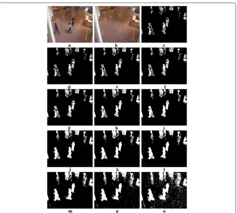
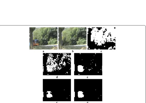
to 6.5025 and 58.5225 as proposed in [36]. In Equation1, l, c, and s represent the luminance, contrast, and struc-ture of two images. In this paper, we computed the SSIM for local regions (e.g., a 3 × 3 block) to eliminate back-ground components. Figure 1a and b show the input and reference background images, respectively. Figure1c and g show the intensity and hue difference images be-tween Figure1a and b, respectively. The SSIM difference image between Figure 1a and b is shown in Figure 1k. Thresholding (if a pixel value of the difference image was larger than the given threshold value, the pixel was eliminated) was applied to the difference images with various threshold values (low, medium, large), and the resulting images are shown in Figure 1d,e,f,h,i,j,l,m,n. For the intensity component (Figure 1c,d,e,f ), the differ-ences between the shadow regions and the correspond-ing background regions were high. The thresholdcorrespond-ing

operation still left shadows when using a low threshold value (e.g., 80). When we used a larger threshold value (e.g., 120) to eliminate the shadows, potential foreground objects were also eliminated (Figure1f ).

For the hue component (Figure 1g,h,i,j), shadows were not retained, but many of the background regions con-tained high difference values. To eliminate these back-ground regions, we tried using a larger threshold value (e.g., 120). However, the top portion of the person with the blue jacket and the red portion of the person on the right were also eliminated. Furthermore, the small object in the lower-left corner was almost deleted when the intensity com-ponent or the hue comcom-ponent was used. However, the method based on the SSIM correctly retained the object (Figure 1k,l,m,n). In the SSIM, global intensity and contrast changes were not determined as forms of distortion [36]. Therefore, the proposed method proved to be robust against shadows with lower intensity values while retain-ing internal structures. Furthermore, since the proposed method used the variances and covariance of two local regions, it could detect objects with similar colors. In

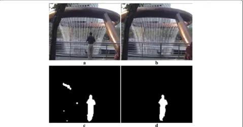
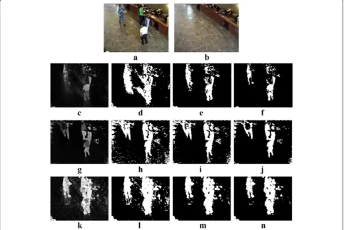
Figure 2a, a person's head color was similar to the back-ground regions. The proposed method showed improved performance compared to the other method [31] (http:// www.na.icar.cnr.it/~maddalena.l/MODLab/SoftwareSOBS. html). Similarly, in Figure 2b, the woman's jacket color was similar to the background regions. The proposed method correctly classified the woman as a foreground object while the other method missed the jacket.

To apply the SSIM to local regions, we used a sliding win-dow approach. For each pixel, we computed the SSIM of a 3 × 3 window centered at the pixel. LetA(i,j) =⌊AR(i,j),AG (i,j),AB(i,j)⌋be a pixel in the RGB color space. Then, the similarity image (SI) between intensity imagesAI(i,j) andBI (i,j) was calculated as follows:

SI_AI_;BIð Þ ¼i;j SSIM AIð Þi;j ;BIð Þi;j

ð2Þ

where

AIð Þ ¼i;j 1

3 A

R_{ð Þ þi;j A}G_{ð Þ þi;j A}B_{ð Þi;j}

;μAI_{ð Þi;j}

¼1

9

X1

v¼−1

X1

u¼−1

AI_{ðiþu;jþvÞ} !

ð3Þ

σ2

AI_{ð Þi;j} ¼

1 9

X1

v¼−1

X1

u¼−1

AIðiþu;jþvÞ2−μAI_{ð Þi;j}

!

;

σ_AI_{ð Þi;jB}I_{ð Þi;j} ¼

1 9

X1

v¼−1

X1

u¼−1

AIðiþu;jþvÞ−μAI_{ð Þi;j}

BIðiþu;jþvÞ−μBI_{ð Þi;j}

!

AI(i,j) represents an intensity value,μ_AI_{ð Þi;j} andμ_BI_{ð Þi;j} are intensity means,σ_AI_{ð Þi;j} andσ_BI_{ð Þi;j} are intensity standard de-viations, andσ_AI_BI_{ð Þi;j} is the intensity covariance.SI_AI_;BIð Þi;j is close to 1 when two window regions were similar.C1and

C1were set to 6.5025 and 58.5225, respectively [36]. By

as-suming that one image was a reference background image, we obtained a binary background image (BBI) by applying a thresholding operation:

BBI_AI_;BIð Þ ¼i;j 0 backgroundð Þif SIAI;BIð Þi;j >T1

1 foreground candidateð Þ otherwise

(

ð4Þ

Figure 2The effect for detecting the objects which are similar with backgrounds. (a)An input image 1,(b)the results of other method [31],(c)the results of the proposed method,(d)an input image 2,(e)the results of other method [31], and(f)the results of the

T1 is a threshold value which was empirically

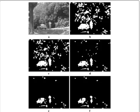
deter-mined and set to 0.55. Figure 3 shows the effect of the threshold value. When we used a small value forT1, most

pixels were classified as background regions (Figure 3c). When we used a large value forT1, most pixels were

clas-sified as foreground regions (Figure 3o). Based on this ob-servation, we setT1to 0.55, though any value between 0.1

and 0.9 provided good performance.

Since we calculated the means and the variances, the computational complexity was low. However, some background pixels were still retained. In order to eliminate the background pixels, we used nonparametric kernel density estimation.

Determining foreground and background areas using KDE Generally, KDE can model multi-modal probability distribu-tions without requiring any prior information. It is effective for modeling the arbitrary densities of real environments. KDE was applied to each pixel of the training images. In other words, we extracted training samples at each pixel lo-cation of the training images. Let s1, s2, …, sN be training

samples and we used the Gaussian kernel function. Then, the probability ofxtwas calculated as follows [21]:

p xð Þ ¼t

1 N

XN

i¼1

1

ffiffiffiffiffiffiffiffi

2πσ

p e−21σðsi−xtÞ2 ð₅Þ

Figure 3The effect of thresholdT1. (a)An input image,(b)the reference background image,(c)T1= 0.1,(d)T1= 0.2,(e)T1= 0.3,(f)T1= 0.35,

where σrepresents the kernel function bandwidth andN is the number of training samples. A pixel was classified as a background pixel if the estimated probability was larger than the given threshold. It was observed that a large value ofNproduced more robust results. Consequently, a typ-ical KDE method requires a large number of operations. On the other hand, we first eliminated most background pixels using the spatial similarity (SS) method and used only two features (one of the RGB components and one of the normalized RGB components). Also, we used a small number of samples (one hundred samples). Therefore, we were able to significantly reduce the computational complexity of the KDE without sacrificing performance. Figure4shows an example of the proposed method. We eliminated most background pixels using the SS method (Figure4c). However, some background pixels were still retained and we eliminated these pixels using KDE. In this case, the candidate pixels made up 5% to 6% of the entire image. The processing time was also reduced accordingly.

Based on this observation, we propose a computation-ally efficient background subtraction method by eliminat-ing background regions useliminat-ing spatial similarity in the spatial domain and the KDE method in the temporal do-main. By combining spatial and temporal features, the proposed method produced better performance than the conventional KDE method. Figure 5 shows the compari-son results. These sequences contain dynamic background

regions. Tree branches were swaying and the curtain was moving in the wind. In dynamic background regions, it is difficult to accurately model the background in the conven-tional KDE method. Therefore, many background com-ponents are often classified as foreground comcom-ponents. However, since most of the background components in the proposed method were eliminated with spatial similarity, most of the background components misclassified as fore-ground components were correctly classified as backfore-ground components.

The proposed method

Determine the background type

The reference background image (RBI) was computed as the average of the training intensity images:

RBIIð Þ ¼i;j 1 N

XN−1

t¼0

AItð Þi;j ð6Þ

where _AI

tð Þi;j represents a pixel of the t-th intensity

image of a video sequence andNis the number of train-ing images, which was set to 100. In other words, the first 100 images of a given video sequence generally were used as training images. We also computed the averages of the RGB channels of the training images:

RBIΩð Þ ¼i;j 1 N

XN−1

t¼0

AtΩð Þi;j where Ω∈fR; G; Bg ð7Þ

Then, a similarity image between the reference back-ground and training intensity images was computed using Equation 2 and the reference binary background image (RBBI) was computed:

For each pixelð Þi;j

r ið Þ ¼;j 1 N

XN−1

t¼0

SI_RBII_;AI tð Þi;j

RBBIð Þ ¼i;j _{1 moving background}0 _ððstatic backgroundÞ_Þ if_otherwiseðr ið Þ;j >0:8Þ

ð8Þ

The RBBI successfully detected moving background com-ponents such as moving escalators, waving tree branches, and water fountains.

Determine the foreground candidate pixels

When a new image was entered, a BBI was computed between the RBI and the input intensity image using Equations 3 to 4. If BBI(i, j) = 1, the pixel could have been either a foreground pixel or a moving background pixel. If RBBI(i, j) = 1 (moving background), we com-puted the difference between the intensity input image and the RBII. If the difference between the input

intensity image and the RBII was small, the pixel could have been a background pixel. Also, the pixel was classi-fied as a foreground candidate when the difference was larger than the given threshold, and the pixel was classified as a foreground candidate if BBI(i,j) = 1 and RBBI(i,j) = 0. The following procedure was used to classify a pixel:

For each pixel i;ð Þj

If BBI_RBII_;II

kð Þ ¼i;j 1

; then

IfðRBBIð Þ ¼i;j 1Þ; then

FCIkð Þ ¼i;j

if RBII_{ð Þi;j−I} kIð Þi;j

_>T2

1 ðforeground candidateÞ otherwise

0 ðbackgroundÞ

8 > > < > > :

Otherwise

FCIkð Þ ¼i;j 1 ðforeground candidateÞ ð9Þ

where FCIk(i,j) represents a candidate image,IIkð Þi;j

rep-resents the k-th input intensity image (see Equation 3),

andT2was empirically set to 30. IfT2was too large, most

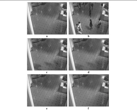
pixels were classified as background pixels. In other words, many foreground pixels were misclassified as back-ground pixels whenT2was too large. Figure 6shows the

results for various values ofT2. Figure6a,b shows an input

image and the BBI. Figure6c,d,e,f shows the FCI for vari-ous values ofT2. Most foreground pixels were eliminated

when T2 was set to 80 (Figure 6f ), while most moving

background pixels were retained when T2 was set to 10

(Figure6c). In order to choose an optimal threshold value, we tested the proposed method with various values ofT2

using some video sequences with dynamic background re-gions and chose the threshold value (T2= 30). At this

point, most background regions were removed.

Subtract the background pixels using KDE

We classified only the foreground candidate pixels (i.e., FCIk(i,j) = 1) using KDE. Since there were high correlations

among the R, G, and B components, and using all three

channels produced only slight improvements, we used only the color with the largest difference. To improve perform-ance, we also used one of the normalized RGB components that were robust against illumination changes and that rep-resented the chrominance information well. We selected one of the RGB component channels as follows:

For each pixelð Þi;j of the k‐th frame If FCIð kð Þ ¼i;j 1Þ

dmax¼ max Diffð R;DiffG;DiffBÞ

ð10Þ

where

DiffR ¼RBIRð Þi;j−IR_kð Þi;j

DiffG¼RBIGð Þi;j −IG_kð Þi;j

DiffB¼RBIBð Þi;j −IB_kð Þi;j

wheredmaxrepresents the maximum difference. LetΩmax

be the channel with the maximum difference.

A foreground candidate pixel was classified as a back-ground pixel when the estimated probability density func-tion of the pixel value was larger than the given threshold as follows:

if 1 N

XN−1

m¼0

1

ffiffiffiffiffiffiffiffi

2πσ

p e− 1 2σ I

Ωmax

k ð Þi;j −AΩmmaxð Þi;j

2

>T3;

decide the pixel as background otherwise;

decide the pixel as foreground

ð11Þ

whereσrepresents the kernel width. Since the probabil-ity densprobabil-ity function of the background pixel was un-known, we assumed that the probability densities for all intensity values were identical. Therefore, we set T3 to

1/256. We used the standard deviation of the training images as the kernel width. This procedure was repeated using the normalized RGB color components, which were computed as follows:

IΩnormalizedð Þ ¼i;j

255_⋅IΩð Þi;j

IR_{ð Þ þi;j I}G_{ð Þ þi;j I}B_{ð Þi;j} withΩ∈fR;G; Bg ð12Þ

whereI(i,j) represents the input image. If either the esti-mated probability density function of the pixel using the original RGB channels or the estimated probability density function of the pixel value of the normalized RGB channels was classified as a foreground component, the pixel was de-termined to be a foreground component. After this proced-ure, there were several small holes inside the foreground regions and some noise elements in the background regions. Most pixel-based methods suffer from this kind of problem. In order to address this, we applied a morphological oper-ation to remove the small holes and noise elements. In par-ticular, we used erosion followed by dilation and then a region filling technique was applied to the results [37].

Updating

After the decision procedure, the RBI and the pixels of the training images had to be updated to adapt to the changing background areas. We used a simple IIR filter to update the RBI as follows [38]:

If pixelð Þi;j is classified as background; RBIΩð Þ ¼i;j ð1−αÞRBIΩð Þ þi;j αIΩ_kð Þi;j where Ω∈fR; G; Bg

ð13Þ

whereαrepresents the learning rate and was set to 0.01. The training images were updated by replacing the old-est pixel with the new background pixel. There is a trade-off in the choice of α. If a value for α was large, the RBI quickly reflected background changes. Figures7

and 8 show the RBI changes for various learning rate values. As can be seen in Figure 7, the RBI was affected by shadows when we used a large value forα. Figure7a, b shows the 372nd input and the initial RBI images. Figure7c shows the RBI image whenαwas 0.6. Because of a large value for α, the RBI was quickly affected by the shadows. If we used a small value forα, the RBI did not quickly reflect background changes.

In some test sequences, the background gradually be-came brighter over a period (Figure 8). The RBI did not reflect this gradual background change with a small value of α (Figure 8c). Thus, we set α= 0.01, and the learning rate was able to handle background changes ad-equately (Figure 8d).

If sudden background changes occurred, the results may have been erroneous. In order to handle such sud-den background changes, we calculated the image inten-sity difference between the input image and the RBI and determined that sudden background changes occurred if the difference was larger than the given threshold:

if 1

Nx⋅Ny X i¼Nx−1;j¼Ny−1

i¼0;j¼0

IIkð Þi;j−RBIIð Þi;j

_>30

!

;

a sudden background change occurs at thek‐th sequence:

ð14Þ

When a sudden background change was detected at the k-th image, we calculated the image differences be-tween the previous 100 images (from the (k-99)-th image to thek-th image) and the RBI. We selected the previous images that had larger frame differences than the thresh-old. The selected images were temporarily used as the training images. If the number of selected images was smaller than 15, all the pixels of the k-th image were classified as background components. However, the RBI was not updated when sudden changes were detected.

Figure 9 shows an example of the proposed background subtraction procedure. Figure 9a is an input image, and Figure 9b shows the reference background image. Figure 9c is the reference binary background image where the white areas represent moving backgrounds (the waving trees). Figure 9d shows the binary background image between Figure 9a and b. Figure 9e shows the foreground candidate image. Figure 9f shows the result obtained using the ori-ginal RGB components, and Figure 9g shows the final re-sult using the normalized RGB components and the morphological operation.

Experimental results

room (MR)) and static background video sequences (shop-ping center (SC), subway station (SS), airport (AP), lobby (LB), bootstrap (B)). The Wallflower's dataset contained various background types (bootstrap (B), camouflage (C), foreground aperture (FA), light switch (LS), moved object (MO), time of day (TD), and waving tree (WT)).

First, we measured the processing time of the proposed method. The proposed method took about 0.015 s per 10,000 pixels, while the processing time of a conventional method [38] was about 1.475 s per 10,000 pixels (using a 2.8-GHz Pentium IV with 1 GB of RAM) when the num-ber of sample images was 100. For instance, the proposed method processed 66.7 frames of video per second when working with 160 × 128 video sequences. The complexity of KDE is OKDE(MN) evaluations (the kernel function,

multiplications and additions), assuming N image pixels andM sample points (Npixels per image andM training images). In the proposed method, we applied ‘spatial si-milarity’to eliminate potential background pixels using

a window processing operation (size of window =w). The computational complexity for calculating spatial similarity is Osimilarity(w2N) operations (multiplications

and additions). Then, the remaining pixels (the number of remaining pixels:K=τN) are further processed using KDE (OKDE(KM)). Therefore, the computational

com-plexity of the proposed method is calculated as follows:

Number of operation¼Osimilarityðw2NÞ þOKDEðKMÞ

¼Osimilarityðw2NÞ þOKDEðτNMÞ

ð15Þ

In the proposed method, the window size is 3 (w= 3), and the average remaining pixels were about 5% ~ 6% of the entire image pixels (τ≅0.05). In other words, the KDE operation was reduced by approximately 95%. Although we needed to compute additional spatial similarity, it had a minor effect on the overall complexity. With 100 train-ing images, the computational complexity for KDE and

Figure 8The RBI images at different values of the learning rate 2. (a)The first input image,(b)the 1,386th input image,(c)the 1,386th RBIIwith theα= 0.001, and(d)the 1,386th RBIIwith theα= 0.01.

the proposed method wasO(100N) andO((9 + 0.05 × 100) N) =O(14N), respectively. In this case, the complexity of the proposed method was about 14% of KDE.

Next, the proposed method was compared with some existing algorithms [31,38-40]. The Jaccard similarity was used as a performance measure [41]:

JS¼ TP

TPþFPþFN ð16Þ

where TP represents the number of true positive pixels, FP represents the number of false positive pixels, and FN represents the number of false negative pixels. Gen-erally, a higher Jaccard similarity index indicates better performance.

Results using Li's dataset

Table 1 shows a performance comparison with Li's data-set based on Jaccard similarity.

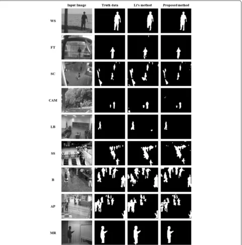
Figure 10 shows the background subtraction results of the proposed method and Li's method using Li's dataset. The first column shows a test image, the second column shows the ground truth data of the test image, the third column shows the results of Li's method, and the fourth column shows the results of the proposed method. Using spatial similarity, the proposed method was robust against shadows. Noticeable improvements were observed in the SC, LB, B, and AP sequences which contained signifi-cant shadows. For these sequences, the proposed method showed about 8.4% ~ 14.9%, 7.8% ~ 20.6%, and 2.91% ~ 12.7% improvement compared to SOBS, Li's method, and Park's method, respectively, in terms of the Jaccard similar-ity. Since the proposed method used covariance, the vari-ances of two local regions, and the normalized RGB color components, it was able to detect some objects that were similar to the background intensity. Therefore, in the WS and the FT sequences that contained objects whose inten-sity values were similar to the background regions, the

proposed method showed improved performance com-pared to the other methods. For instance, a main difficulty of the WS sequence was detecting a person's leg when the intensity value of the leg was similar to the background in-tensity value. The other methods missed parts of the leg while the proposed method accurately detected the leg. For this WS sequence, the proposed method showed about 10.4%, 7.8%, and 2.91% improvements compared to SOBS, Li's method, and Park's method. A main difficulty of the FT sequence was that a person's pants color was similar to the background region when the person stood against the fountain. For the FT sequence, the Jaccard similarity of the proposed method was 0.820, and the proposed method showed about 16.5%, 14.6%, and 10.3% improvements compared to SOBS, Li's method, and Park's method, re-spectively. However, some sequences (e.g., CAM, SS, and MR) contained complex dynamic background sequences. For instance, in the CAM sequence, the background in-cluded tree branches that were constantly swayed by a strong wind. The SS sequence contained moving escala-tors and the MR sequence contained moving curtains). In these kinds of dynamic background sequences, Park’s method (in CAM, SS, and MR) and Li's method (in MR) performed slightly better than the proposed method.

Results using Wallflower's dataset

Table 2 shows a performance comparison with Wallflower's dataset based on FP + FN. Figure 11 shows the results of the proposed method and Wallflower method using the Wallflower's dataset. The first column shows a test image, the second column shows the ground truth data of the test image, the third column shows the results of Wallflower method, and the fourth column shows the results of the proposed method. The proposed method showed notice-able improvements for the C and B sequences. In the B se-quence, the proposed method successfully detected objects that were similar to the background areas. On the other hand, since some moving trees of the WT sequence were classified as foreground components, the proposed method was not as good as Park's method. The LS sequence con-tained a sudden background change and the proposed method showed better performance. In the MO sequence, the proposed method classified the relocated objects (the chair and the phone) as foreground components. To han-dle this kind of problem, higher level processing such as that used in the Wallflower method might be required. The proposed method missed an object whose color was similar to that of the background area in the TD sequence.

The effects of thresholds

Next, we investigated the effects of thresholds (T1andT2

in Equations 8 to 9). Figure 12 shows the Jaccard similarity of the proposed method as theT1andT2values increased

with Li's dataset and wallflower's dataset. In order to

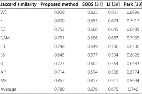
Table 1 Performance comparison with Jaccard similarity (Li's dataset)

Jaccard similarity Proposed method SOBS [31] Li [39] Park [38]

WS 0.929 0.825 0.851 0.8999

FT 0.820 0.655 0.674 0.7917

SC 0.752 0.668 0.645 0.6485

CAM 0.791 0.696 0.683 0.7935

LB 0.798 0.649 0.706 0.6706

SS 0.645 0.577 0.534 0.6826

B 0.723 0.602 0.564 0.6483

AP 0.714 0.594 0.508 0.6774

MR 0.852 0.817 0.911 0.8994

analyze the effect of T1, we computed the false positive

ratio (FPR) and false negative ratio (FNR) metrics as follows:

FPR¼ FP

TPþFPþFN

FNR¼ FN

TPþFPþFN

ð17Þ

When we used a large value for T1, most foreground

pixels were correctly classified as foreground pixels. However, many background pixels also were classified as

foreground pixels. Therefore, FPR increased and FNR decreased. When we used a small value for T1, most

background pixels were classified as background pixels. However, many foreground pixels were classified as back-ground pixels. Therefore, FPR decreased and FNR in-creased when we used a small value for T1. Figure 13

shows the Jaccard similarity, and the FPR and FNR metrics with various values forT1(T2was fixed and set at 30).

We selected the optimal value for T1 and T2. When

we set T1 and T2to 0.55 and 30 respectively, the

fore-ground candidate pixels were about 5% of the entire

number of pixels, and the Jaccard similarity of the pro-posed method was about 0.78 with Li's dataset and the FP and FN numbers were about 6,888 with Wallflower's dataset. Experiments with various values of T1 and T2

show that the proposed method produced stable per-formance when the value ofT1was from 0.5 to 0.65 and

the value ofT2was from 25 to 35.

Conclusions

In this paper, we proposed a background subtraction method that utilized structural similarity, which was ro-bust against various background areas. The proposed method also significantly reduced the level of computa-tional complexity since most pixels were eliminated using the similarity image. We tested the proposed method with two datasets and then compared the pro-posed method with some existing methods. The experi-mental results demonstrated that the proposed method

Table 2 Performance comparison with the number of false positive and false negative pixels (Wallflower's dataset)

FP + FN Proposed method Wallflower [40] Park [38]

C 325 2,395 1,492

WT 487 2,876 249

LS 1,140 1,322 2,260

MO 1,263 0 1,423

TD 685 986 306

FA 2,105 969 2,743

B 883 2,390 1,643

Sum 6,888 11,478 10,116

Figure 12The effects of thresholds (T1andT2).

was effective for various background scenes and com-pared favorably with some existing algorithms.

Competing interests

The authors declare that they have no competing interests.

Authors’information

Sangwook Lee received the BS and MS degrees in electrical and electronic engineering from Yonsei University, Seoul, Repiblic of Korea in 2004 and 2006, respectively. He is currently working toward the PhD degree from Yonsei University and a senior engineer at Samsung Electronics Co. Ltd., Republic of Korea. His research interests include machine vision, image/signal processing, and video quality measurement.

Chulhee Lee received the BS and MS degrees in electronic engineering from Seoul National University in 1984 and 1986, respectively, and a PhD degree in electrical engineering from Purdue University, West Lafayette, Indiana, in 1992. In 1996, he joined the faculty of the Department of Electrical and Computer Engineering, Yonsei University, Seoul, Republic of Korea. His research interests include image/signal processing, pattern cognition, and neural networks.

Acknowledgements

This work was supported by grant no. R01-2006-000-11223-0 from the Basic Research Program of the Korea Science & Engineering Foundation.

Received: 3 July 2013 Accepted: 2 June 2014 Published: 19 June 2014

References

1. NJB McFarlane, CP Schofield, Segmentation and tracking of piglets in images. Mach. Vision App.8(1), 187–193 (1995)

2. MH Hung, CH Hsieh, Speed up temporal median filter for background subtraction, inProceedings of the PCSPA, vol. 1(Harbin, 2004), pp. 297–300 3. F Cheng, S Huang, S Ruan, Advanced motion detection for intelligent video

surveillance systems, inProceedings of the ACM SAC, vol. 1(984, Sierra, 2010), pp. 983–984

4. S Cohen, Background estimation as a labeling problem, inProceedings of ICCV, vol. 2(Beijing, 2005), pp. 1034–1041

5. C Wren, A Azarbayejani, T Darrell, A Pentland, Pfinder: Real-time tracking of the human body. IEEE Trans. Pattern Anal. Mach.19(7), 780–785 (1997) 6. M Zhao, J Bu, C Chen, Robust background subtraction in HSV color space,

inProceedings of SPIE MSAV, vol. 1(Boston, 2002), pp. 325–332

7. X Pan, Y Wu, GSM-MRF based classification approach for real-time moving object detection. J. Zhejiang Univ. Sci. A9(2), 250–255 (2008)

8. C Rambabu, W Woo, Robust and accurate segmentation of moving objects in real-time video, inProceedings of International Symposium on Ubiquitous VR, vol. 191(Yanji City, 2006), pp. 65–69

9. C Stauffer, E Grimson, Adaptive background mixture models for real-time tracking, inProceedings of IEEE Conf. Computer Vision Patt. Recog, vol. 2

(Fort Collins, 1999), pp. 246–252

10. W Zhang, X Fang, X Yang, Q Wu, Spatiotemporal Gaussian mixture model to detect moving objects in dynamic scenes. J. Electron. Imaging16(2), 023013-1–023013-6 (2007)

11. T Su, J Hu, Background removal in vision servo system using Gaussian mixture model framework, inProceedings of ICNSC, vol. 1(Singapore, 2004), pp. 70–75 12. A Doulamis, Dynamic background modeling for a safe road design, in

Proceedings of PETRA, vol. 1(Samos, 2010), pp. 1–9

13. MH Khan, I Kypraios, U Khan, A robust background subtraction algorithm for motion based video scene segmentation in embedded platforms, in

Proceedings of FIT, vol. 1(Abbottabad, 2009), pp. 1–8

14. H Wang, P Miller, Regularized online mixture of Gaussians for background with shadow removal, inProceedings of AVSS, vol. 1(Klagenfurt, 2011), pp. 249–254

15. SC Wang, TF Su, SH Lai, Detection of moving objects from dynamic background with shadow remova, inProceedings of ICASSP, vol. 1

(Prague, 2011), p. 925

16. L Zhao, X He, daptive Gaussian mixture learning for moving object detection, inProceedings of IC-BNMT, vol. 1(Beijing, 2010), pp. 1176–1180 17. Z Bin, Y Liu, Robust moving object detection and shadow removing based

on improved Gaussian model and gradient information, inProceedings of ICMT2010, vol. 1(Ningbo, 2010), pp. 1–5

18. HH Lim, JH Chuang, TL Liu, Regularized background adaptation: a novel learning rate control scheme for Gaussian mixture modeling. IEEE Trans. Image Process.20(3), 822–836 (2011)

19. H Zhou, X Zhang, Y Gao, P Yu, Video background subtraction using improved adaptive-K Gaussian mixture model, inProceedings of ICACTE, vol. 5(Chengdu, 2010), pp. 363–366

20. J Suhr, H Jung, G Li, J Kim, Mixture of Gaussians-based background subtraction for Bayer-pattern image sequences. IEEE Trans. Circuits Syst. Video Technol.21(3), 365–370 (2011)

21. A Elgammal, D Harwood, L Davis, Non-parametric model for background subtraction, inProceedings of ECCV, vol. 1(Dublin, 2000), pp. 751–767 22. T Tanaka, A Shimada, D Arita, R Taniguchi, A fast algorithm for adaptive

background model construction using Parzen density estimation, in

Proceedings of IEEE Conf. AVSS, vol. 1(London, 2007), pp. 528–553 23. A Tavakkoli, M Nicolescu, G Bebis, Automatic robust background modeling

using multivariate non-parametric kernel density estimation for visual surveillance, inProceedings of the International Symposium of Advances in Visual Computing LNCS, vol. 1(Nevada, 2005), pp. 363–370

24. N Martel-Brisson, A Zaccarin, Unsupervised approach for building non-parametric background and foreground models of scenes with significant fore-ground activity, inProceedings of VNBA, vol. 1(Vancouver, 2008), pp. 93–100 25. B Han, DCY Zhu, L Davis, Sequential kernel density approximation through

mode propagation: applications to background modeling, inProceedings of ACCV, vol. 1(Jeju, 2004), pp. 1–6

26. G Gordon, T Darrell, M Harville, J Woodfill, Background estimation and removal based on range and color, inProceedings of CVPR, vol. 1

(Fort Collins, 1999), pp. 2459–2464

27. A Monnet, A Mittal, N Paragios, V Ramesh, Background modeling and subtraction of dynamic scenes, inProceedings of ICCV, vol. 2

(Beijing, 2003), pp. 1–8

28. H Kim, R Sakamoto, I Kitahara, T Toriyama, K Kogure, Robust foreground extraction technique using Gaussian family model and multiple thresholds, inProceedings of ACCV, vol. 1(Tokyo, 2007), pp. 758–768

29. Q Zhu, G Liu, Z Wang, H Chen, Y Xie, A novel video object segmentation based on recursive kernel density estimation, inProceedings of ICINFA, vol. 1

(Shenzhen, 2011), pp. 843–846

30. A Kolawole, A Tavakkoli, Robust foreground detection in videos using adaptive color histogram thresholding and shadow removal, inProceedings of ISVC, vol. 2(Las Vegas, 2011), pp. 496–505

31. L Maddalena, A Petrosino, A self-organizing approach to background subtraction for visual surveillance applications. IEEE Trans. Image Process.

13(4), 1168–1177 (2008)

32. L Maddalena, A Petrosino, Self organizing and fuzzy modelling for parked vehicles detection, inProceeding of ACVIS, vol. 1(Bordeaux, 2009), pp. 422–433

33. H Lin, T Liu, J Chuang, A probabilistic SVM approach for background scene initialization, inProceedings of ICIP, vol. 3(Rochester, 2002), pp. 893–896 34. L Cheng, M Gong, D Schuurmans, T Caelli, Real-time discriminative

background subtraction. IEEE Trans. Image Process.20(5), 1401–1414 (2011) 35. I Junejo, A Bhutta, H Foroosh, Dynamic scene modeling for object

detection using single-class SVM, inProceeding of International Conference on Image Processing, vol. 1(Hong Kong, 2010), pp. 1541–1544

36. Z Wang, AC Bovik, HR Sheikh, EP Simoncelli, Image quality assessment: from error visibility to structural similarity. IEEE Trans. Image Process.13(4), 1–14 (2004) 37. R Gonzalez, R Woods,Digital Image Processing, 2nd edn. (Prentice Hall,

Englewood Cliffs, 2002)

38. JG Park, C Lee, Bayesian rule-based complex background modeling and foreground detection. Opt. Eng.49(2), 027006-1–027006-11 (2010) 39. L Li, W Huang, IYH Gu, Q Tian, Statistical modeling of complex backgrounds

for foreground object detection. IEEE Trans. Image Process.13(1), 1459–1472 (2004)

40. K Toyama, L Krumm, B Brumitt, B Meyers, Wallflower: principles and practice of background maintenance, inProceedings of IEEE ICCV, vol. 1(Kerkyra, 1999), pp. 255–261

41. P Jaccard, The distribution of flora in the alpine zone. New Phytol.

11(2), 37–50 (1912)

doi:10.1186/1687-5281-2014-30