A closed form unwrapping method for a spherical omnidirectional view sensor

R E S E A R C H

Open Access

A closed form unwrapping method for a

spherical omnidirectional view sensor

Nguan Soon Chong, Yau Hee Kho and Mou Ling Dennis Wong

Abstract

This article proposes a novel method of image unwrapping for spherical omnidirectional images acquired through a non-single viewpoint (NSVP) omnidirectional sensor. It has three key steps i.e. (1) calibrate the camera to obtain parameters describing the spherical omnidirectional sensor, (2) map world points onto mirror points and,

subsequently, onto image points, and (3) set up the projection plane for the final image unwrapping. Based on the projection plane selected, the algorithm is able to produce three common forms of unwrapping, namely cylindrical panoramic, cuboid panoramic, and ground plane view using closed form mapping equations. The motivation for developing this technique is to address the complexity in using a NSVP omnidirectional sensor and ultimately encouraging its application in robotics field. One of the main advantages of a NSVP omnidirectional sensor is that the mirror can often be obtained at a lower price as compared to the single viewpoint counterpart.

Keywords: Omnidirectional view sensor, Spherical mirror, Non-single viewpoint, Omnidirectional view image unwrapping

1 Introduction

The omnidirectional view sensor has gradually emerged as a popular and effective vision sensor in the field of robotics. In most cases of application, the large field of view (FOV) provided by the sensor allows simultaneous monitoring of the surrounding in different view angles and therefore enables a more flexible and responsive algo-rithmic behaviour. Among the several configurations, the catadioptric version has received relatively more attention than its dioptric counterpart. Rees [1] first suggested that a hyperboloidal mirror mounted on a perspective camera

would enable a 360◦ FOV on the camera. Subsequently,

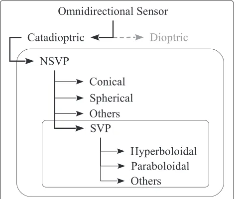
it was realised by Yamazawa et al. [2] and concurrently several other types of mirror profile were also introduced, such as conical [3], spherical [4], and paraboloidal [5].a_A summary of the omnidirectional view sensor classification is provided in Figure 1.

However, as a trade-off for a large FOV, the mirror’s curvature causes an unfavourable distortion in omni-directional images. Therefore, a pre-processing termed

“unwrapping”, is often necessary for a

perspectively-*Correspondence: [email protected]

Faculty of Engineering, Computing, and Science, Swinburne University of Technology (Sarawak Campus), Kuching, Sarawak, Malaysia

correct alteration on the image acquired. Mirrors with a single viewpoint (SVP) property [5,6] such as hyper-boloidal, parahyper-boloidal, and a specifically designed mirror [7] for example, can be represented by a common sphere model [8] that allows effective and unified camera cali-bration techniques [9-18] or otherwise by approximation models [19,20]. These calibration methods subsequently allow unwrapping on the images acquired. For instance, one of the approaches was presented by Lei et al. [21], where they had demonstrated two forms of panoramic unwrapping—cylindrical and cuboid.

Calibration on non-SVP (NSVP) mirror profiles, such as those of conical and spherical, usually require spe-cific modelling based on the particular mirror shape used [22-24], by approximation model [22,23,25], or otherwise, for example, by the use of polarised imaging [26]. NSVP mirrors are popular choices of catadioptric omnidirec-tional sensors due to the immediate availability and lower cost, particularly for the spherical one. Further evaluation on the advantage of spherical mirror profile is provided in Section 2. Among the earlier related works on NSVP omnidirectional image unwrapping, Gaspar et al. [27,28] had worked on unwrapping of spherical omnidirectional images into ground plane view (bird’s eye view). Later, Jeng and Tsai [29] proposed a mirror-invariant technique

Figure 1Classification of omnidirectional view sensor.The common catadioptric omnidirectional sensor mirror profiles with practical SVP solution are the hyperboloidal and paraboloidal ones. The category “others” in the figure refers to profiles that are not of conic section. Spherical and conical are the common NSVP mirror profiles. Note that the SVP mirror profile is also a subset of NSVP. If the requirement of SVP constraint is not met, they fall back to NSVP category. Dioptric is another category of omnidirectional sensors beyond the discussion scope of this paper.

for panoramic unwrapping by means of ground-truth information calibration.

In this article, a closed-form solution for spherical omnidirectional image unwrapping incorporating advan-tages from the different techniques is presented. Dif-ferent from previous works, the proposed unwrapping technique (1) does not require any prior knowledge on sensor parameters or ground-truth information, (2) pro-duces output that scales accordingly with the resolution of the image, (3) utilises closed form forward and back-ward mapping equations, and (4) is designed for multiple output forms such as cylindrical panoramic view, cuboid panoramic view, and ground plane view unwrapping.

The proposed approach attempts ray tracing of the light source in the surrounding captured by the camera of the omnidirectional sensor. By acquiring the mathematical model that describes the direction of ray, the desired form of unwrapping can be achieved by choosing an appropri-ate 3D projection plane. There are essentially three stages of procedure required in order to complete the unwrap-ping. The first stage requires the perspective camera of the omnidirectional system to be calibrated and thus an equivalent radius and height of the spherical mirror can be geometrically deduced based on the resolution of the image. The second stage would make use of the param-eters to provide a closed-form analytical solution to the

ray tracing of the imaging system that enables correspond-ing mappcorrespond-ing of world points and their equivalent image points. The last stage of the procedure is to set up the pro-jection plane of the unwrapped image in a 3 dimensional (3D) space.

The rest of the article is organised as follows: In Section 2, the use of a spherical mirror profile is justified despite the complexity introduced, and in Sections 3, 4, and 5, the three key stages are explained. In Section 6, issue on the output quality of the algorithm is discussed. Conclusion of the work is provided in Section 7. Finally, Appendix pro-vides detailed derivations of several important equations used in this article.

2 Evaluation on a spherical omnidirectional sensor

Similar to other NSVP mirror profiles, the spherical mir-ror profile is often unfavourable in various applications that require mapping between an image point and its corresponding unwrapped counterpart due to the lack-ing of a practical solution for SVP formation. However, the benefit of utilising the spherical mirror should not be overlooked as it may provide an omnidirectional sensor solution that is justifiably more practical at present. Firstly, a spherical object with a polished surface is easily acces-sible and so the cost is reasonably low as compared to other SVP mirror profiles because they are mostly custom made using computer numerical control (CNC) machine. Strictly speaking, a SVP formation has rather demanding requirements, which if not met, would render the SVP property of the mirrors an approximation at best. There-fore for most of the time, they are practically of NSVP setting.

Secondly, as a para-catadioptric sensor is not affected by vertical translational error in fabrication [5,6], the spher-ical mirror is invariant to rotational error up to a certain degree because it is rotationally symmetrical in all axes as illustrated in Figure 2. Apart from that, since it is not crucial to maintain a specific distance between a NSVP mirror and the camera’s effective focal point along the optical axis, the spherical mirror is also invariant to trans-lational error along the optical axis. In short, the design constraint for a spherical omnidirectional sensor is more relaxed and can tolerate fabrication error.

Thirdly, parameters describing a spherical model are as minimal as two parameters—its radius and its position on the optical axis. As compared to other more complex shapes, its parameter calibration is theoretically simpler and straight forward as described in Section 3.

3 Stage 1-camera calibration

Prior to ray tracing, calibration is needed to estimate the two parameters describing the spherical mirror—radius,

Figure 2Spherical mirror’s toleration on rotational error.A spherical mirror is technically a hemisphere. The other half is usually not useful therefore is rarely incorporated into the sensor design. Since the viewing angle does not encompass the complete hemisphere, it can often tolerate rotational error up to a certain degree,θ. The vertical dash line represents the optical axis.

centre,h. Perspective cameras are generally modelled as shown in Figure 3. The parameters describing the model are usually grouped and termed as the intrinsic parame-ters. These information is useful in mapping the relation-ship between an image pixel and its corresponding world point in 3D space.

At present, methods to calibrate the intrinsic param-eters of SVP omnidirectional cameras with the mirror attached are well established as reported in [10,19,30,31]. For NSVP mirror profiles such as those of conical and

Figure 3Perspective camera model.A perspective camera can be modelled by the intrinsic parameters. An optical axis passes through the centre of projection,C, and the principal point,c, that lies on the perpendicular image plane,I. The distance betweenCandcis termed focal distance,f.

spherical, a unified calibration algorithm requires polar-isation imaging [26] for instance. However, since the sphere has only two parameters, it can be easily deduced from a calibrated camera instead [24], such as by the use of Zhang’s [32] method. Subsequently, the camera’s intrinsic parameter,K, can be obtained in the following form:

K= ⎡ ⎢ ⎣

fx s uo 0 fy vo

0 0 1

⎤ ⎥

⎦ (1)

where f are the focal distances with subscript x and y

denoting the respective axes,sis the skew of pixel, andc=

[uo,vo]T is the principal point. Without any loss of gen-erality, a sensor with rectangular pixel is assumed where

s=0. In practice, the actual sensor in perspective camera may not be necessarily square and will therefore introduce an aspect ratio as infy/fx. However, the two focal distances are often very similar renderingfy/fx≈1. With negligible margin of error, we have treatedfx=fyin our application, and avoided extra computation to correct the input image due to a non 1:1 aspect ratio. The calibrated result of the perspective camera is shown in Table 1. For brevity,fxand

fyare subsequently denoted byf.

When a sphere is projected onto an image plane, a circu-lar feature is obtained as shown in Figure 4. The calibrated

f is useful in estimating the radius of the spherical mirror based on the resolution of input image. The ground-truth radius of the sphere is not necessary because with limited quality of the input image, the resolution of the unwrapped image should be logically sufficient based on the resolution of the input image. Therefore, we establish the existence of a virtual sphere, assuming to be located at a constrained distance intersecting the image plane based

on the calibrated f. R and h are then remapped from

Figure 4 onto the virtual sphere as illustrated in Figure 5. Prior to parameter estimation, the radius of the circu-lar feature,ρ, on the image plane is first estimated using Hough Circle Transform [33]. Geometrically, it is

under-stood that ρ = R as illustrated in Figure 5. Due to

the viewing angle,ζ, of the perspective projection from

C, certain portion of the actual spherical mirror/virtual sphere will not appear on the image plane. To estimate

the remapped R, two assumptions are made where (1)

the centre of the spherical mirror, therefore the centre of

Table 1 Calibrated values of the intrinsic parameters of the perspective camera in pixels

Parameter Calibrated value (pixel)

f 1216.09±8.68

fy/fx 1.00±0.02

c uo 335.59±8.37

Figure 4Projection of sphere on image plane.When a sphere is projected onto an image plane, a circular feature is obtained. The parameterRdescribes the spherical mirror’s radius whilehis the distance between the spherical mirror and the centre of projection,C. However, the radius of the circular feature does not represent an equivalent radius of the sphere due to the viewing angle,ζ.

the virtual sphere, coincides the optical axis, and (2) the spherical mirror is at least a “hemisphere” visible to the perspective camera. Although the first assumption may not be necessarily true as fabrication error will always results in misalignment, it is a reasonable approximation [15,19,20,29] and will later greatly simplify the coordi-nate mapping in Section 4. The remappedRandhcan be derived by the method of similar triangles as follows:

R= ρ fl=ρ

1+t2 ₍₂₎

h=l2_+R2_=l1+t2 ₍₃₎

l= f2_+ρ2 _t=tanζ

2 =

R l =

ρ

f

From Equations (2) and (3),√1+t2_{is easily observed} as a correction factor for the parameters. The estimatedR

andhwill be useful in completing the mapping of world points to equivalent image points, and vice verse. The estimated parameter values for our spherical mirror are shown in Table 2.

In Table 2, the estimated principal point, which is the centre of the circular feature on the image plane obtained using Hough Circle Transform, is easily translated into the centre of the virtual sphere. The error introduced when comparing with that from the intrinsic parameter calibra-tion in Table 1 is marginal. Since the assumpcalibra-tion that the optical axis coincides with the centre of the virtual sphere was made, the estimated principal point from Table 2 is used instead of those from Table 1.

Figure 5Real world image acquisition model.The actual perspective camera collects light rays that enter its effective pupil introduced by a perspective lens. The intensity of the light rays is then measured by the CCD/CMOS sensor plane placed behind the effective pupil. Distance of the effective pupil to the sensor plane is the effective focal length. The effective pupil is equivalent to the centre of projection,C, of the perspective camera model where the image plane,I, can be imagined to be located further behind the sensor plane at the distance of its focal distance,f, formingIflipped. As shown in the figure, the perspective camera model is placed overlapping the real world image acquisition figure with the image plane placed in front of the centre of projection. Based on the obtained focal distance, an equivalent virtual sphere mirror is visualised to be intersecting the image plane at a constrained distance,h. The projection of the sphere on the image plane can also be visualised as a compressed version of the virtual sphere. Note that parameterRandhare remapped from the actual spherical mirror (in Figure 4) onto the virtual sphere.

4 Stage 2-mapping of points

For a typical catadioptric omnidirectional sensor, incident rays would make contact with the mirror, be reflected with respect to the normal axis at the contacted mirror sur-face, and subsequently enter the pupil of the perspective

Table 2 Calibrated values of the intrinsic parameters of the perspective camera in pixels

Parameter Estimated value (pixel)

R 205.83

h 1246.58

c uo 345

camera. Figure 5 illustrates the actual image acquisition of a perspective camera at the presence of an effective pupil and effective focal length introduced by a perspec-tive lens with the perspecperspec-tive camera model overlapping over. The perspective camera model has an equivalent structure where the centre of projection is analogous to the effective pupil. With this constraint, ray tracing from the image plane to an equivalent world coordinate is made possible. The image plane in an actual perspective cam-era is logically located behind the effective pupil but in the perspective camera model, it has been placed in front of the centre of projection. This is useful so that the image pixels are not mathematically flipped in both axes and the common image coordinate system can be applied directly for pixel referencing.

In Section 3, an assumption has been made where the spherical mirror’s centre coincides with the optical axis and subsequently the geometry of light ray made is assumed to be rotationally symmetrical about the optical axis. Therefore within a 3D space where points are repre-sented in Cartesian form ofPx,y,zwith the optical axis labelled as z-axis, ρ = (x2_+y2_{) can be introduced to} reduce the dimension of our problem into that of a 2D. Without any loss of generality, we position our origin at the centre of the virtual sphere. Figure 6 illustrates the important geometry used for subsequent derivations with a reduced dimensionality.

Figure 6Important geometry for mapping functions derivation. The corresponding relationship between an arbitrary world point,Pw, mirror point,Pm, image point,Pi, and caustic point,Pc, in theρ−z plane are provided by the caustic curve and mirror parameters. Important geometry for equation derivation is also illustrated.

In general, the point mapping process is a two-step translation process. The first two-step translates points between image and mirror while the second step trans-lates points between mirror and world. Mirror points are points on the spherical mirror where lights are reflected while world points are the points of light source in the 3D space. In subsequent derivations, variables with subscript

i, m, c, and w represent their respective image, mirror, caustics and world component. The idea of caustic is dis-cussed in Section 4.2. For brevity, functions that map in the order ofPito Pm toPware subsequently denoted as “forward mapping functions” whereas the reversed coun-terparts are denoted as “backward mapping functions”.

Similar derivations of such a point mapping process had been previously attempted. Micusik and Pajdla [22,23] had not provided a closed-form two-way translation but relied on numerical search for the backward mapping func-tion. That had been addressed by Agrawal et al. [24] in an approach which is rather comparable to our method. They had shown that the backward mapping is achiev-able via a forth order equation while we have employed a sixth order one due to a tight integration with the caustic geometry. However, on the forward mapping, our approach involves less operations to complete with 11 additions/subtractions, 23 multiplications/divisions, and 3 square roots (2 square roots for cylindrical unwrap-ping) instead of 38 addition/subtraction, 55 multiplica-tions/divisions, and 2 square roots as in [24]. While both of our mapping functions operate in the same

P(ρ,z) space, Agrawal et al. [24] derivations useP(ρ,z) space in the forward mapping but Px,y,z space in the backward mapping. Thus, our approach provides an advantage in cylindrical unwrapping that has a constantρw.

4.1 Mapping between image point and mirror point

The reflected light from the mirror is assumed to pass through the centre of projection of the perspective cam-era model (which is analogous to the camcam-era pupil). In Figure 6, an arbitrary mirror point, Pm(ρm,zm), and its corresponding image point,Pi

ρ_i,f, are illustrated as the intersection points of the reflected light made with the virtual spherical mirror and the image plane, respectively. The backward mapping function ofρ_i , given thatPm is known, is straight forward by using the method of similar triangles:

ρi=

f h−zm

ρm (4)

the equation of the virtual sphere, s(ρ)=R2_−ρ2_.

Geometrically, mk and ck can be easily identified

as −fρi and h, respectively. Equating both equations

at ρ=ρi yields a quadratic equation as shown in

Equation (5).

k(ρ_i)=s(ρ_i)

mkρi+ck= R2−ρi2

m2_k+1ρ2_i +(2mkck) ρi+

c2_k−R2=0 (5)

ρm=

fh− −h2_ρ2

i +f2R2+ρi2R2

f2_+ρ2 i

ρi (6)

Mathematically, the other of solution of Equation (5) is always larger than Equation (6) and therefore is rejected by observing the geometry of the intersections. Subse-quentlyzm can be obtained either froms(ρ)ork(ρ)as follows:

zm=s(ρm)= R2−ρ2m (7)

4.2 Mapping between mirror point and world point

In [5,6,34], caustics of several NSVP omnidirectional sen-sors were extensively reviewed. A caustic is defined as the locus of viewpoints forming a surface that is tangen-tial to the incident rays. The centre of projection of the perspective camera model is analogous to the effective pupil of the camera, therefore a virtual caustic is applied onto the virtual sphere defined in Section 3. Assum-ing that the spherical mirror’s centre coincides with the

optical axis, the caustic surface is rotationally symmetri-cal about the optisymmetri-cal axis and is therefore reduced to a

curve inρ −zplane. Before subsequent mapping

func-tions can be derived, the caustic model has to be first investigated.

4.2.1 Caustic curve

A general model for caustic curve that is compatible for all conic section mirror profiles has been provided by Swaminathan et al. [34]. However, since the generalisation is not important for our application, we opt for a simpler model derived specifically for a spherical mirror provided by Baker and Nayar [5,6].

The parametric equations for the spherical mirror

caus-tic curve are derived in [5,6] assuming R = 1. In

order to serve our purpose, the parametric equations

have been reformulated with R as a parameter instead.

Firstly, an incident ray reflected at a mirror point

Pm(ρm,zm) =

ρ_m,R2_−ρ2 m

is described by a straight line equation, j(ρm), and this is repeated for point P_m(ρm+dρm,zm+dzm). Secondly, the intersec-tion point ofj(ρm) andj(ρm+dρm)is obtained by tak-ing the limit dρ_m → 0 while applying a constraint on

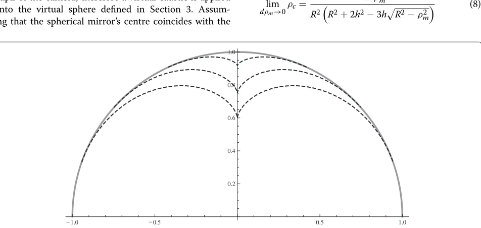
dz with (ρ_m+dρ_m)2+ (zm+dzm)2 = R2. Denoting a point on the caustic curve asPc(ρc,zc), the result of the derivation is shown in Equations (8) and (9). Detailed derivations can be found in Appendix. Figure 7 shows sample plots of the caustic curve of a spherical mir-ror with = 1 described in parametric equations with varyingh.

lim dρm→0

ρc=

2h2_ρ3 m

R2_R2_+2h2_−3hR2_−ρ2 m

(8)

1.0 0.5 0.5 1.0

0.2 0.4 0.6 0.8 1.0

zc=

h−R6_+hR2_R2_−ρ2 m

2ρ2 m+3R2

+h2_4ρ4

m−2ρ2mR2−2R4

R2_R2_+2h2_−3hR2_−ρ2

m R2−2h

R2_−ρ2 m

(9)

4.2.2 Point mapping

The forward mapping function ofPm to its correspond-ing world point,Pw(ρw,zw)is obtained by differentiating Equations (8) and (9) with respect toρm using the chain rule of calculus. This thus forms the gradient,mj, of the incident ray,j(ρ). However, due to the lost of depth infor-mation during the image acquisition process, constraint on either zw or ρw is needed. Mathematically, the con-straint is needed becausej(ρ)is valid forρ=(ρ_m,∞). In practical application however, a constraint onρwis better thanzwbecause at certainρm,mjwill change sign. More discussion is provided in Section 6. Assumingρwis to be constrained,zwis then given by:

zm−zw ρm−ρw =

mj=

dzc

dρm

dρ_c

dρm

zw=zm−(ρm−ρw)

dzc

dρ_m

dρ_c

dρ_m

(10)

where mj is derived from the caustic curve provided in Equation (13).

In order to derive the backward mapping functions of

Pw to its corresponding Pm, more measures have to be

taken. An incident ray would pass through a Pw and

is tangential to the caustic curve at Pc. This relation-ship can be exploited as a sixth order polynomial shown in Equation (11). Detailed derivation can be found in Section 4.3.

16h4z_w2+ρ_w2ρ_m6 −16h4R2ρw

ρ_m5

+4h2R2h2R2+2hR2zw+−8h2+2R2z2w

+−8h2+2R2ρ_w2ρ_m4 +4h2R46h2−R2−2hzwρwρ3m +R4−4h4R2+h2R4 +−8h3R2+2hR4zw

+−4h2+R22z2_w+20h4−12h2R2+R4ρ_w2ρ_m2

−2hR64h2−R2(h−zw) ρwρm

−R64h4−5h2R2+R4ρ_w2=0

(11)

By solving Equation (11), the correspondingρmcan be obtained andzm=

R2_−ρ2

mcan be determined

accord-ingly. Since 0≥ρm ≥ρm,max, there will only be one valid solution for Equation (11).ρm,maxis easily observed as the

maximumρm due to the maximum viewing angle,ζ, as

follows:

tanζ

2 =

ρm,max

R =

√ h2_−R2

h

ρm,max=R 1− R h 2 (12)

4.3 Derivation of world-to-mirror mapping function In order to derive Equation (11), it is first considered that an incident ray passes through a Pw(ρw,zw)and is tan-gential to the caustic curve at Pc(ρc,zc). Therefore, the mapping of aPwto its correspondingPm(ρm,zm)can be done by making use of the gradient of the incident ray,

mj, which can be obtained by differentiating Equations (8) and (9) with respect to ρ_m using the chain rule of calculus.

mj= zc−zw

ρc−ρw

= dzc dρm

_d

ρc dρm

(13)

= hR4+R4

R2_−ρ2 m+2h2

2ρ_m2 −R2 R2_−ρ2 m ρm

R4_+4h2_(ρ2 m−R2)

(14)

Substituting Equations (8) and (9) into Equation (13) and subsequently rearranging them would then yield Equation (15). By discarding the denominator of Equation (15), the square root functions are then eliminated form-ing Equation (16).

R4

h(ρw−ρm)+

R2_−ρ2

mρw−ρmzw

+2h22ρ_m2ρ_w−R2ρ_w−ρ_mR2 R2_−ρ2

m+2ρmzw

R2−ρ_m2

ρmR4+4h2ρm2 −R2

=0 (15)

Finally, not shown in this article due to the length of the equation, Equation (16) is summed to a common denominator and subsequently the denominator is again discarded. Collecting theρ_mterms hence forms Equation (11).

−R2+ρ_m2 +

−hR4_ρ

m+4h2R2zwρm−R4zwρm−4h2zwρm3 +hR4ρw ₂

−2h2_R2_ρm−2h2_R2_ρw+R4_ρw+4h2_ρ2

mρw2 =

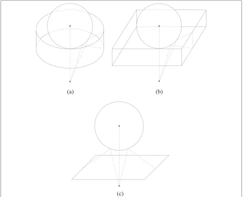
5 Stage 3-projection plane for unwrapping A virtual projection plane is assumed to be an imagi-nary 2 dimensional (2D) plane of light source. The illu-minated light from the plane would travel towards the virtual sphere and thus be reflected into the camera’s pupil. By using the forward mapping functions derived in Section 4, the corresponding incident ray of a specific image point can be traced, and subsequently a world point where the incident ray coincides with the virtual projec-tion plane can be obtained. Then, the backward mapping functions will be used to populate the virtual plane using common interpolation technique (i.e. bilinear interpola-tion). Finally, the plane itself results into an unwrapped image. In addition, by selecting the shape and position of the virtual plane, different forms of unwrapping is pos-sible. Lei et al. [21] had documented the idea of virtual plane in details and they had demonstrated two forms of panoramic unwrapping—cylindrical and cuboid. Cuboid panoramic unwrapping is done by replacing the cylindri-cal virtual plane with a cuboid one. For our case, we will demonstrate that a ground plane view is also possible with our method by choosing an appropriate projection plane as illustrated in Figure 8c.

In order to take advantage of a unified platform with multiple form unwrapping output capability, the map-ping functions have been conveniently made to accept and produce points in the Cartesian form. Therefore, the loca-tion of each element in a virtual plane (ends up as an image pixel) described in Cartesian points would be eas-ily translated into their respective image points. Generally, a lookup table of corresponding points will be generated so that subsequent unwrapping can be speeded up. Such practice is commonly applied in omnidirectional image unwrapping field and is documented in details in Jeng and Tsai [29] work.

5.1 Cylindrical panoramic unwrapping

Cylindrical panoramic unwrapping can be done using an open-ended cylinder plane wrapping around the spherical mirror as shown in Figure 8a. Since a cylinder is rota-tionally symmetrical about its central axis and by letting it coincides with the optical axis, points on the pro-jection plane described in cylindrical coordinate system (e.g.(ρ,ϕ,z)) will have a similar mapping ofρandzfor all ϕ. Therefore, only one set of mapped coordinate is required.

The cylinder will have a user-defined radius in pixel,rk, and thus the width of the unwrapped image is roughly

2πrk pixel. The height of the cylinder is dependent on the region of image to be unwrapped and is also user-defined. Due to the nature of the spherical mir-ror, unwrapping is only suitable up to a certain region of the mirror. More will be discussed in Section 6. Figure 9a shows the set-up of our experiment in a

controlled environment. The captured image is shown in Figure 9b with cylindrical panoramic unwrapping shown in Figure 10.

5.2 Cuboid panoramic unwrapping

Cuboid panoramic unwrapping is an enhanced version of the cylindrical one. As documented in [21], a cuboid pro-jection plane will artificially create a perspective view of the surrounding. The output of this method results in a more natural view of the surrounding for human eye perception and is particularly effective if the surrounding is a rectangularly confined space. Figure 11 is the result of unwrapping Figure 9b using cuboid projection plane as illustrated in Figure 8b. The result shown assumed a cuboid placed at the centre of the virtual plane with upright orientation to thex-axis butx-axis but in practice, a rectangular one would work equally well. The shape, position, and orientation of the cuboid projection plane is mainly dependant on the boundary of surrounding space (e.g. walls, partitions, building etc.).

5.3 Ground plane view unwrapping

Ground plane view unwrapping generates an output that appears perspectively correct as if the image were cap-tured from some height above. A more commonly known term for ground plane view is thebird’s eye view. As the name suggests, ground plane view unwrapping is mainly used to detect features on the ground. While panoramic unwrapping can include ground features, they would introduce low quality unwrapping due to insufficient data point (image pixel) near the centre of the mirror and rendering less useful interpolated data. Previous work by Hicks and Bajcsy [35] performed analogue ground plane correction using a specialised mirror profile. Another work by Gaspar and Santos-Victor [27] corrects distortion on ground feature by solving the geometry made by the captured light rays.

In Figure 12, a controlled environment to demonstrate ground plane view unwrapping is set up. To adapt to such form of unwrapping using the existing derived map-ping functions, a projection plane that is normal to the optical axis is simply placed some distance away from the virtual sphere instead of upright project planes used in the previous two panoramic unwrapping schemes as shown in Figure 8c. Illustration of the result is shown in Figure 13.

5.4 Assessment on accuracy

Figure 8Projection planes for unwrapping.By choosing an appropriate projection plane, the algorithm is able to produce different unwrapped views, including (a) the cylindrical panoramic view, (b) the cuboid panoramic view, and (c) the ground-plane view.

Figure 10Cylindrical panoramic unwrapping.Common cylindrical unwrapping can be done using an open-ended cylindrical virtual plane.

5.4.1 Line fitting

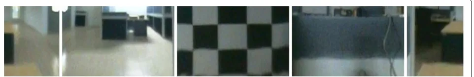
In this experiment, a checker-box pattern was initially captured and unwrapped into cuboid panoramic view. Then, Harris and Stephens [36] corner detection algo-rithm was used to capture the corner points in the unwrapped checker-box pattern. For any ambiguities due to detection of multiple corners at the same point, the cen-troid of the cluster was used instead. Subsequently, hori-zontal and vertical lines were fitted using linear regression model to the points as shown in Figure 14. Note that for vertical lines, the axes were flipped so that fitting is possible. Throughout the entire process, human interac-tion was made minimal where user only specifies the total points to detect and a coarse estimation of the location of the points.

In Table 3, an analysis of the line-fitting in Figure 14b is presented. The mean gradient suggested the “straightness” of the fitted lines while meanR2suggested the “goodness” of fit of the points involved. As can be seen, the mean gra-dient and meanR2approach 0 and 1 respectively, which imply a proportionally high degree of correctness in the relative position of the points involved as they are mapped from omnidirectional view to cuboid panoramic view. A second analysis was done on the spacing,, between the

fitted lines. Let y be the mean spacing of horizontal

lines whilexbe mean spacing of vertical lines, the ideal benchmark checker-box pattern of Figure 14a should pro-duce a ratio of y

x = 1 neglecting lens distortion. On the unwrapped checker-box pattern, it is found that y

x=0.93, indicating an error of 7% in the ratio after unwrapping.

This simple line fitting experiment was meant to show a preliminary assessment of the mapping functions without

involving complex algorithm. Since it is not a common practice in previous works, a benchmark for the result in Table 3 is not possible. Thus, another experiment that is more commonly conducted, i.e. 3D reconstruction in Section 5.4.2, was carried out to provide further evalua-tion on the mapping funcevalua-tions.

5.4.2 3D reconstruction

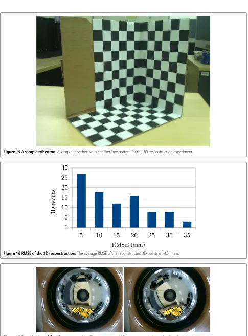
In this experiment, a 3D reconstruction [37] of a trihe-dron with checker-box pattern was conducted. Initially, two images of the trihedron in Figure 15 were captured from two different viewing locations and unwrapped into cuboid form. Then, a total 92 pairs of corresponding points from the two views were sampled manually. From the corresponding points, the fundamental matrix was first computed and subsequently the two camera matrices, P1andP2, associated with the two views were deduced. As P1is set at [I|0], this resulted in a projective reconstruc-tion of the corresponding points by linear triangulareconstruc-tion method. Finally, the reconstructed 3D points are upgraded to a metric reconstruction [37].

From the reconstructed trihedron points, several mea-surements were obtained to assess the accuracy of the mapping equations. Figure 16 shows the distribution of the calculated root-mean-square error (RMSE) of the 3D points with an average of 14.54 mm. Without further opti-misation on the reconstruction (i.e. bundle adjustment), the error obtained is observed to be within a similar range as previous works [20,22]. Finally, the 3D points were reprojected back to the input image as shown in Figure 17 and the reprojection error of the points were measured as shown in Figure 18. The average reprojection error of the 3D points was found to be 0.22 pixels.

(a)

(b)

Figure 12Experiment set-up for ground plane view unwrapping.A controlled environment for ground plane view unwrapping is set up as in (a)and a corresponding omnidirectional view image is captured as shown in(b).

(a)

(b)

Figure 14Accuracy assessment of mapping functions.Horizontal and vertical lines are fitted on a checker-box pattern unwrapped into cuboid panoramic view as in(b)to assess the accuracy of the mapping functions.(a)is the same pattern taken using a perspective view camera.

5.4.3 Sources of error

The assessments on accuracy revealed a certain degree of error introduced by the mapping functions. The pos-sible sources of error include the assumptions made in the derivations of the mapping functions. An ideal spher-ical mirror is assumed in the derivations while this may not be always true in practice. Also, the spherical mir-ror’s centre might not coincides with the optical axis perfectly. Factors such as these could also affect the

accuracy of parameter calibration for f and R, which

eventually lead to error compounding as mapping is processed.

Other than that, the lens of the camera could be ideally assumed to provide a perfect perspective view projec-tion. Slight fish-eye distortion might be introduced as the omnidirectional view image is captured. Lastly, sampling error, either manually or using Harris corner detection algorithm [36], is inevitable.

6 Image quality and algorithm limitation

Due to heavy dependency on ray tracing in the proposed algorithm, different unwrapping forms are optimum only in certain regions on the omnidirectional image that is radially confined from the centre of the mirror. For ground plane view unwrapping, incident rays withmj≤0 do not intersect anx−yplane placed below the virtual sphere, which translates tomk ≥ 0 for reflected rays. Theoret-ically, unwrapping cannot be done with the mentioned condition. In practical unwrapping however,mjwill never reach 0 but converges to it. At the converging region, there is insufficient data point at the input image (image pixel) to

Table 3 Analysis of line fitting on Figure 14b

Line MeanR2 Mean Gradient Spacing,(px)

Mean σ

Horizontal 1.00 -0.01 23.12(x) 1.19

Vertical 1.00 -0.01a _24.73

y 2.06

The axes are flipped to allow proper fitting, thus a value closing to 0 indicates a “straighter” vertical line fitting.

perform useful interpolation that results in highly detailed output and therefore should be avoided. Figure 19 shows a plot of ρ_i versus ρ_win pixels, where ρ_i gradually con-verges to a limit as ρw progresses, indicating thatρw is roughly represented by similarρi as the projection plane expands. The converging region suggests a low quality output region.

For panoramic unwrapping, upright projection planes suffer less from the above mentioned limitation. As shown in the solid line plot in Figure 20, ρi is rather evenly “distributed” acrosszwindicating that the output is inter-polated from a rather evenly spaced data point. However, for practical usage, as points on the input image are rep-resented using Polar coordinates, region closing to the centre of the mirror should be avoided as it is stretched along the angular axis after unwrapped, which produces an output with degraded quality.

Also note in Figure 20, an overlapping dashed line plot is provided for the purpose of showing thatmj changes sign during the complete mapping. In Section 4.2.2, as Equation (10) is derived, there is a need to provide addi-tional constraint on eitherρworzw. Mathematically, ifρw is constrained, there might be two possible correspond-ingzwdepending on the sign ofmjat that instance. One of thezwwould be invalid by observing the geometry. In forward mapping, this means that an arbitraryzwmay not have a corresponding valid solution ofρw. For practical implementation, constraint onρwcan be effectively pro-vided by the projection plane and thus the consideration made when deriving Equation (10).

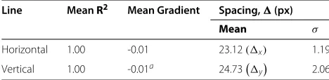
Figure 15A sample trihedron.A sample trihedron with checker-box pattern for the 3D reconstruction experiment.

Figure 16RMSE of the 3D reconstruction.The average RMSE of the reconstructed 3D points is 14.54 mm.

Figure 18Reprojection error of the 3D reconstruction.The average reprojection error of the reconstructed 3D points is 0.22 pixel.

7 Conclusion

A novel technique of unwrapping for spherical omnidi-rectional images has been proposed. The algorithm com-prises three key stages in which (1) the camera is first calibrated to obtain essential parameters, (2) ray tracing is then utilised to solve the functions that map points back and forth between the omnidirectional image and its unwrapped counterpart, and finally (3) a projection plane is set up for the unwrapping.

The proposed unwrapping scheme enables three com-monly performed unwrapping forms, namely, cylindrical panoramic, cuboid panoramic, and ground plane view to be done. The different forms of unwrapping can be achieved by selecting an appropriate projection plane to be populated as the unwrapped image.

Finally, the accuracy of the mapping functions was accessed by conducting a simple line fitting and a 3D

Figure 19ρiversusρwgraph for ground plane unwrapping.For ground plane unwrapping,ρigradually converges to a limit asρw progresses in pixels. The converging region suggests a degraded quality output region whereρware roughly represented by similarρi as the projection plane expands.

reconstruction. The line fitting experiment showed a 7% error in the checker-box pattern ratio. For the 3D reconstruction experiment, the average RMSE was 14.54 mm while the average reprojection error was 0.22 pixel.

Appendix

Derivation of a spherical mirror’s caustic curve In order to derive the caustic curve for a spherical mir-ror, the gradient of an incident ray,j(ρ,ρ_m) = mj(ρm)· ρ+cj(ρm)at an arbitrary mirror point,Pm(ρm,zm), is first derived. Note that for clarity,mjandcjare functions ofρm whereasjis a function ofρandρ_m. Prior to this section, they are omitted for brevity. Figure 6 shows thatmj(ρm) is in fact tanθ whereθ =α−2β.

mj(ρm)=tanθ =tan(α−2β)

= tan(α)tan(β)2+2 tan(β)−tan(α)

tan(β)2−2 tan(α)tan(β)−1

(17)

tanα= h−zm

ρ_m =

h−R2_−ρ2 m

ρ_m (18)

tanβ= −d[s(ρ)]

dρ _ρm = ρ_m

R2_−ρ2 m

, (19)

where tanα can be deduced geometrically while tanβ

can be obtained from the gradient of the spherical mir-ror curve,s(ρ). Substituting Equations (18) and (19) into Equation (17) yields:

mj(ρm)= −

R2R2_−ρ

m2−hR2+2hρm2 2hρm

0 100 200 300 400 500 600 50

100 150 200

3.00 2.00 1.00 0.00 1.00 2.00

zw

i

m

j

Figure 20ρiversuszwgraph andmhversuszwgraph for upright plane unwrapping.For upright plane unwrapping,ρiis rather “evenly distributedacrosszwas illustrated by the solid line plot (Both are in pixels). Therefore, panoramic unwrapping suffer less quality degradation due to mapping alongρ-axis. The overlapping dashed line plot illustrates the gradient of incident ray,mj, involved. Sincemjchanges sign at one point, the constraint for Equation 10 is more convenient whenzwis chosen.

Secondly, thez-intercept ofj(ρ,ρ_m),cj(ρm), is obtained by examine the relationship ofzm=j(ρm,ρm).

zm=j(ρm,ρm)=mj(ρm)·ρm+cj(ρm)

which implies that:

cj(ρm)=zm−mj(ρm)·ρm

=ρm

R2R2_−ρ

m2−hR2+2hρm2

2hρ_mR2_−ρ

m2−ρmR2

+R2_−ρm2

(21)

Thirdly, let two incident rays contacting atPm(ρm,zm) and P_m(ρ_m+dρ_m,zm+dzm), their intersection points would form the caustic curve. Points on the caustic curve are denoted asPc(ρc,zc).

zc=j(ρc,ρm)=j(ρc,ρm+dρm)

mj(ρm)·ρc+cj(ρm)=mj(ρm+dρm)·ρc+cj(ρm+dρm)

ρc=

cj(ρm+dρm)−cj(ρm) mj(ρm)−mj(ρm+dρm)

(22)

Substituting Equations (20) and (21) into Equation (22) and taking the limit ofdρm → 0 thus results in Equation (8). Accordingly,zcis therefore derived fromj(ρc,ρm) =

mj(ρm)·ρc+cj(ρm), yielding Equation (9).

Endnote

a_{Paraboloidal catadioptric camera and hyperboloidal}

catadioptric camera are also known as para-catadioptric and hyper-catadioptric respectively in short mainly due to extensive utilisation.

Abbreviations

FOV: field of view; SVP: single viewpoint; NSVP: non-single viewpoint; CNC: computer numerical control; 3D: 3 dimensional; 2D: 2 dimensional; RMSE: root-mean-square error.

Competing interests

The authors declare that they have no competing interests.

Acknowledgements

This research project is funded by the Ministry of Higher Education (MOHE), Malaysia, under a Fundamental Research Grant Scheme

(FRGS/2/2010/TK/SWIN/03/02). N. S. Chong also thanks the Swinburne University of Technology (Sarawak Campus) for his Ph.D. studentship.

Received: 22 June 2012 Accepted: 11 December 2012 Published: 11 January 2013

References

1. DW Rees, Patent 3505465 (1970)

2. K Yamazawa, Y Yagi, M Yachida, inProceedings of the 1993 IEEE/RSJ

International Conference on Intelligent Robots and Systems ’93, IROS ’93,

vol. 2. Omnidirectional imaging with hyperboloidal projection, (Tokyo, Japan, 1993), pp. 1029–1034

3. Y Yagi, S Kawato, vol. 1. Panorama scene analysis with conic projection, (1990), pp. 181–187

4. J Hong, X Tan, B Pinette, R Weiss, EM Riseman, Image-based homing. IEEE Control Syst.12, 38–45 (1992)

5. S Baker, SK Nayar, A theory of single-viewpoint catadioptric image formation. Int. J. Comput. Vis.35(2), 175–196 (1999). http://www. springerlink.com/index/WU62M18P65412043.pdf

6. S Baker, SK Nayar, inProceedings of the Sixth International Conference on

Computer Vision, 1998. A theory of catadioptric image formation (Bombay,

India, 1998), pp. 35–42

7. W Sturzl, W Srinivasan, inProccedings of the OMNIVIS - 10th Workshop on

Omnidirectional Vision, Camera Networks and Non-classical Cameras.

Omnidirectional imaging system with constant elevational gain and single viewpoint (Zaragoza, Spain, 2010), pp. 1–7

8. C Geyer, K Daniilidis, inProceedings of the 6th European Conference on

Computer Vision-Part II , ECCV ’00. A unifying theory for central panoramic

systems and practical applications, (London, UK, 2000), pp. 445–461. http://dl.acm.org/citation.cfm?id=645314.649434

9. JP Barreto, H Araujo, Geometric properties of central catadioptric line images and their application in calibration. IEEE Trans. Pattern Anal. Mach. Intell.27, 1327–1333 (2005). http://dl.acm.org/citation.cfm?id=1070616. 1070819

10. X Ying, Z Hu, Catadioptric camera calibration using geometric invariants. IEEE Trans. Pattern Anal. Mach. Intell.26(10), 1260–1271 (2004) 11. X Ying, H Zha, in2005 IEEE/RSJ International Conference on Intelligent

Robots and Systems, 2005. (IROS 2005). Simultaneously calibrating

catadioptric camera and detecting line features using Hough transform (Alberta, Canada, 2005), pp. 412–417

12. P Vasseur, EM Mouaddib, inBritish Machine Vision Conference. Central catadioptric line detection (Kingston University, London, UK, 2004)

13. C Mei, P Rives, inIEEE International Conference on Robotics and Automation, 2007. Single view point omnidirectional camera calibration from planar grids, (Roma, Italy, 2007), pp. 3945–3950

14. L Puig, Y Bastanlar, P Sturm, JJ Guerrero, JA Barreto, Calibration of central catadioptric cameras using a DLT-Like approach. Int. J. Comput. Vis.93, 101–114 (2011)

15. XM Deng, FC Wu, YH Wu, An easy calibration method for central catadioptric cameras. Acta Automatica Sinica.33(8), 801–808 (2007) 16. S Gasparini, P Sturm, J Barreto, in2009 IEEE 12th International Conference

on Computer Vision. Plane-based calibration of central catadioptric

cameras, (2009), pp. 1195–1202

17. F Wu, F Duan, Z Hu, Y Wu, A new linear algorithm for calibrating central catadioptric cameras. Pattern Recogn.41(10), 3166–3172 (2008) 18. Y Wu, Z Hu, inTenth IEEE International Conference on Computer Vision, 2005.

ICCV 2005, vol. 2. Geometric invariants and applications under

catadioptric camera model, (Beijing, China, 2005), pp. 1547–1554 19. D Scaramuzza, A Martinelli, R Siegwart, inProceedings of the 2006 IEEE/RSJ

International Conference on Intelligent Robots and Systems. A toolbox for

easily calibrating omnidirectional cameras, (Beijing, China, 2006), pp. 5695–5701

20. D Scaramuzza, A Martinelli, R Siegwart, inIEEE International Conference on

Computer Vision Systems, 2006 ICVS ’06. A flexible technique for accurate

omnidirectional camera calibration and structure from motion, (New York, USA, 2006), p. 45

21. J Lei, X Du, YF Zhu, JL Liu, Unwrapping and stereo rectification for omnidirectional images. J. Zhejiang Univ. SCI. A.10(8), 1125–1139 (2009). http://www.springerlink.com/index/10.1631/jzus.A0820357

22. B Micusik, T Pajdla, inProceedings of the 2004 IEEE Computer Society

Conference on Computer Vision and Pattern Recognition, 2004, CVPR 2004,

vol. 1. Autocalibration 3D reconstruction with non-central catadioptric cameras, (Washington, DC, USA, 2004), pp. 58–65

23. B Micusik, T Pajdla, Structure from motion with wide circular field of view cameras. IEEE Trans. Pattern Anal. Mach. Intell.28(7), 1135–1149 (2006) 24. A Agrawal, Y Taguchi, S Ramalingam, inProceedings of the 11th European

conference on computer vision conference on Computer vision: Part III.

Analytical forward projection for axial non-central dioptric and catadioptric cameras (ECCV’10, Springer-Verlag, Berlin, Heidelberg, 2010), pp. 129–143

25. S Derrien, K Konolige, inProceedings of IEEE Workshop on Omnidirectional

Vision, 2000. Approximating a single viewpoint in panoramic imaging

devices, (South Carolina, USA, 2000), pp. 85–90

26. A Shabayek, O Morel, D Fofi, inThe Proceedings of the 10th Workshop on Omnidirectional Vision (OMNIVIS) in conjunction with Robotics Systems and

Science RSS. Auto-calibration and 3D reconstruction with non-central

catadioptric sensors using polarization imaging (Zaragoza, Spain), p. 2010 27. J Gaspar, J Santos-Victor, inProceedings of the International Symposium on

Intelligent Robotic Systems - SIRS’99. Visual path following with a

catadioptric panoramic camera (Coimbra, Portugal, 1999). http:// citeseerx.ist.psu.edu/viewdoc/summary?doi:10.1.1.33.3379 28. N Winters, J Gaspar, G Lacey, J Santos-Victor, inProceedings of the IEEE

Workshop on Omnidirectional Vision. Omni-directional vision for robot

navigation, (South Carolina, USA, 2000), pp. 21–28

29. SW Jeng, WH Tsai, Using pano-mapping tables for unwarping of omni-images into panoramic and perspective-view images. IET Image Process.1(2), 149–155 (2007)

30. C Geyer, K Daniilidis,Catadioptric camera calibration, vol. 1. (Kerkyra, Greece, 1999), pp. 398–404

31. C Geyer, K Daniilidis, Paracatadioptric camera calibration. IEEE Trans. Pattern Anal. Mach. Intell.24(5), 687–695 (2002)

32. Z Zhang, A flexible new technique for camera calibration. IEEE Trans. Pattern Analy. Mach. Intell.22(11), 1330–1334 (2000). http://dx.doi.org/10. 1109/34.888718

33. RO Duda, PE Hart, Use of the Hough transformation to detect lines and curves in pictures. Commun. ACM.15, 11–15 (1972)

35. RA Hicks, R Bajcsy, Reflective surfaces as computational sensors. Image Vis. Comput.19(11), 773–777 (2001). http://linkinghub.elsevier.com/ retrieve/pii/S0262885600001049

36. C Harris, M Stephens, inProceedings of Fourth Alvey Vision Conference. A combined corner and edge detector, (Manchester, UK, 1988), pp. 147–151 37. RI Hartley, A Zisserman,Multiple View Geometry in Computer Vision, 2nd

edn. (Cambridge University Press, Cambridge, 2004)

doi:10.1186/1687-5281-2013-5

Cite this article as:Chonget al.:A closed form unwrapping method for a

spherical omnidirectional view sensor.EURASIP Journal on Image and Video Processing20132013:5.

Submit your manuscript to a

journal and benefi t from:

7Convenient online submission

7Rigorous peer review

7Immediate publication on acceptance

7Open access: articles freely available online

7High visibility within the fi eld

7Retaining the copyright to your article