Applying compressive sensing to TEM video: a substantial frame rate increase on any camera

R E S E A R C H

Open Access

Applying compressive sensing to TEM video:

a substantial frame rate increase on any camera

Andrew Stevens

, Libor Kovarik

, Patricia Abellan

, Xin Yuan

, Lawrence Carin

and Nigel D. Browning

Abstract

One of the main limitations of imaging at high spatial and temporal resolution duringin-situtransmission electron microscopy (TEM) experiments is the frame rate of the camera being used to image the dynamic process. While the recent development of direct detectors has provided the hardware to achieve frame rates approaching 0.1 ms, the cameras are expensive and must replace existing detectors. In this paper, we examine the use of coded aperture compressive sensing (CS) methods to increase the frame rate of any camera with simple, low-cost hardware modifications. The coded aperture approach allows multiple sub-frames to be coded and integrated into a single camera frame during the acquisition process, and then extracted upon readout using statistical CS inversion. Here we describe the background of CS and statistical methods in depth and simulate the frame rates and efficiencies for

in-situTEM experiments. Depending on the resolution and signal/noise of the image, it should be possible to increase the speed of any camera by more than an order of magnitude using this approach.

Mathematics Subject Classification: (2010) 94A08·78A15

Keywords: Compressive sensing; Transmission electron microscopy; Video; Coded aperture; Nanoparticles; Chemical dynamics

Background

In-situ transmission electron microscopy (TEM) has established itself as a very powerful analytical technique for its ability to provide a direct insight into the nature of materials under a broad range of environmental condi-tions. With the recent development of a wide range of in-situTEM stages and dedicated environmental TEM, it is now possible to image materials under high-temperature, gas, and liquid conditions, as well as in other complex electrochemical, optical, and mechanical settings [1–4]. In many of these applications, it is often critical to capture the dynamic evolution of the microstructure with a very high spatial and temporal resolution. While enormous developments in electron optics and the design ofin-situ cells have been made, leading to significant improvements in achievable resolution [5–7], there still exist many chal-lenges associated with capturing dynamic processes with high temporal-resolution.

*Correspondence: [email protected]

1Pacific Northwest National Laboratory, Richland, WA, USA 2Duke University ECE, Durham, NC, USA

At the present time, a majority of in-situTEM video capture is performed with charge-coupled device (CCD) cameras. High-performance commercially available CCD cameras have readout rates in the range of a few tens of MB/s [8], which under appropriate binning conditions can provide video acquisition rates (∼30 ms acquisition rate) [8]. Important progress has been made recently by the introduction of the direct detection camera (DDC), which utilizes CMOS technology, and thus provides an order of magnitude increase of the readout rate— it has been demonstrated that these cameras can be operated in the ms range [9]. Importantly, DDCs pro-vide a new approach by directly recording the incoming electrons without the use of a scintillator. By avoid-ing the electron-to-light conversion, the DDC achieves unprecedented sensitivity. While improving temporal res-olution, the DDC also enables electron dose reduction, another key challenge forin-situTEM imaging. The lim-itation in implementing this technology (or any other hardware-based acquisition system), however, is that as the frame rates increase, reading out the images becomes a challenge—the issue then becomes a data transfer prob-lem rather than an electron detection probprob-lem.

CS combines sensing and compression in one operation, and thus provides an approach that could further improve the temporal resolution of any detector (both CCDs and DDCs). Because the signal is measured in a compressive manner, fewer total measurements are required; which, when applied to TEM video capture, improve the acqui-sition speed and reduces the electron dose rate. CS is a recent concept and has come to the forefront due the seminal works of Candès et al. [10] and Donoho [11]. Since those publications, there has been enormous growth in the application of CS and development of CS vari-ants. The concept of CS has also been recently applied to electron tomography [12] and reduction of electron dose in scanning transmission electron microscopy (STEM) imaging [13].

The approach proposed in this paper increases the effec-tive frame rate of any camera by adding a mask/aperture between the sample and the imaging sensor. The mask is moving at a fixed rate so that a sequence of coded images is integrated into a single frame on the sensor. Once the experiment has concluded, the data can be decompressed by the algorithm presented here or by other methods such as GAP [14] or TwIST [15]. The approach presented here is also useful for imaging dose-limited materials. A traditional camera would capture a single image that has integrated a sequence of undamaged and damaged images, whereas CS-TEM would capture a sequence of coded images that can be reconstructed to determine the precise onset of beam damage.

In addition to presenting new results, this article is meant to serve as a general introduction to CS and also to the methods behind the algorithm presented herein, which is fundamentally different from previ-ous approaches. Many of the references are tutorials and reviews (e.g., [16–21]), while others highlight recent developments (e.g., [22–24]). We hope that the descrip-tions and illustradescrip-tions provide a starting point for micro-scopists to enter the related literature.

Before presenting the experimental results, CS the-ory and a probabilistic recovery approach are reviewed. Next, theinexpensivemicroscope modifications needed to achieve this imaging approach are outlined. In the exper-iments section, simulated recovery results are shown for palladium nanoparticle oxidation and silver nanoparticle coalescence. Finally, for both simulations, image degrada-tion is quantified as a funcdegrada-tion of compression level, and an estimate for a reasonable compression level is given.

Methods

CS has quickly become one of the most important discov-eries in the digital age. The theory of CS, and numerous implementations, shows that a signal can be compressed at the time of measurement and accurately recovered at a later time in software. In imaging applications, the

compression can be applied spatially to reduce the num-ber of pixels that need to be measured. This can lead to an increase in sensing speed, a decrease in data size, and dose reduction in the case of electron microscopy [13]. In video applications, the time dimension can be com-pressed. By compressing the sensed data in time, the total frame rate of a camera system is multiplied by integrating a sequence of coded images into a single frame from the camera. In this section, the statistical models and micro-scope hardware for an approach to compressively sensing and recovering videos will be described.

The traditional approach in signal acquisition is to sam-ple and then compress. This is motivated by the Nyquist-Shannon sampling theorem, which states that in order to accurately reconstruct a signal it must be sampled at a frequency at least twice the highest frequency present. Figure 1 shows a sum of three sine waves with differ-ent frequencies and amplitudes. By the sampling theorem, a rate of at least 128 would be required to reconstruct the signal. Yet, in the frequency domain, three samples are sufficient; the signal is said to be 3-sparse under the Fourier basis. One notion of the CS problem is to design a non-adaptive sensing scheme to measure signals in the basis that makes the signal as sparse as possible— effectively reducing the number of measurements below the Nyquist rate [18]. This approach has the benefit of eliminating the overhead of sensing the entire signal according to the sampling theorem. Usually the basis is chosen to be Fourier modes or wavelets, but it is also pos-sible to discover the basis from the measurements [25].

CS background

In imaging problems, the signal has two spatial dimen-sions, so the basis must also have two spatial dimensions.

0 0.1 0.2 0.3 0.4 0.5 0.6 0.7 0.8 0.9 1 −2 −1 0 1 2 Time Amplitude

0 10 20 30 40 50 60 70

0 0.2 0.4 0.6 0.8 1

Frequency (2πω)

Normaliz

ed Ma

gnitude

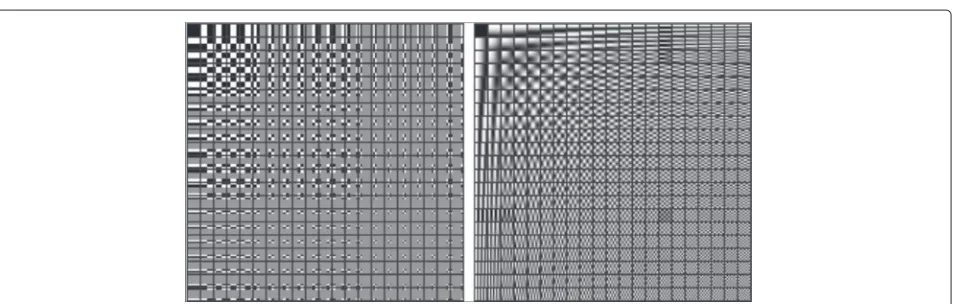
Often, small two-dimensional images (and higher) are referred to as patches. Figure 2 shows the two-dimensional Haar wavelet basis alongside the discrete cosine basis (DCT)—the real part of the Fourier trans-form. The basis patches along the top and left sides are the same as the one-dimensional basis elements, except they have been copied to fill the second dimension. The interior of the table is formed by combining the basis patches along the top and left edges into all of the possible two-dimensional variants.1

There are conditions on the design of the sensing scheme2, but in practical applications and in this paper the sensing scheme will simply omit pixels randomly. The measurements are linear so they can be represented as a matrixand the true signal as a vectorx(flattened from the two-dimensional image). Expressed mathematically,

y=x. (1)

In order to omit pixels, there is a single 1 in each column; another way of stating this is that the rows are randomly selected from the identity matrix without replacement. The representation in Fig. 3 includes zero rows for illustra-tive purposes, but the sensing matrix does not have those zero rows. Because the sensing matrix is missing rows, it is short and wide, that isi ∈ RQ×P,Q P, whereQis the dimension of compressed measurement,y∈RQ, and Pis the dimension of the signalx∈RP. The inverse prob-lem of recoveringxfromyis underdetermined, so further assumptions must be imposed to guarantee a solution.

Equation (1) is somewhat deceiving in that it appears that a single signal is recovered from a single measure-ment. In fact, there is a set of measurements,{y₁,. . .,y_N}, a set of sensing matrices,{1,. . .,N}, and a set of signals {x1,. . .,xN},3with the indexiadded to Eq. (1),

y_i=ixi. (2)

In sensing problems where the signal is an image, the sig-nals{x1,. . .,xN}are patches from the full image. Usually the patches are overlapping so that each pixel has a cor-responding patch, except for the right and bottom regions of the image. Figure 4 is an illustration of the patches and how they overlap. The sensing matrices, measurements, and signals are all obtained by extracting patches from the corresponding full-size images. In the case of the signal, the CS algorithm will recover the patchesxiand then the patches are put back together and the overlapping pixels are averaged.

Dictionary learning and sparse-CS

Dictionaries are another choice for the basis, but dictio-naries do not have an analytical form like the Fourier or wavelet bases. Dictionary learning is a method to discover a frame4from the data, which is referred to as the dic-tionary. The learned dictionary allows every patch to be represented by a weighted sum of a few5 dictionary ele-ments or vectors (assuming overcompleteness). Because the overcomplete dictionary model enforces the use of only a few basis patches, the data is sparse under the dictionary. This approach is advantageous because the learned dictionary can guarantee a sparse representation, whereas choosing a Fourier basis, for example, does not guarantee sparsity. Two learned dictionaries are depicted in Fig. 5.

The first algorithm for dictionary learning was based on human vision [26]. More recently, a much faster vari-ant was proposed, theK-SVD algorithm [27], and Mairal et al. have further improved theK-SVD-based approach and given a thorough review of dictionary learning [16]. Another approach, a part of the approach in this paper, is beta-process factor analysis (BPFA) [25]. BPFA has been used in compressive sensing of STEM images [13]. The relationship between optimization/maximum likeli-hood (K-SVD) approaches and Bayesian/sampling (BPFA)

Fig. 3By turning the image patches into vectors, the sensing scheme can be written as a matrixthat omits pixels when applied to a patch. The vectorei∈RPhas a one in theith position and zeros in all other positions, sohas a subset of identity matrix columns. The illustration shows that the first pixel is eliminated while the second is kept. The zero columns are used here to motivate the idea, but in the actual sensing matrix, the zero columns are not present, so the compressed patch vector (y∈RQ_{) is shorter than the signal patch vector (x∈R}P_,QP)

approaches is discussed after the details of the BPFA model are introduced.

Another approach that has been applied in image restoration tasks, and specifically to STEM image restora-tion is the non-local means algorithm [16, 28]. Non-local means uses all of the image patches simultaneously to find a reweighting of the central pixel of each patch. Sparse representation, on the other hand, finds a sub-set of elements from a dictionary and the corresponding weights to reconstruct an entire patch (dictionary learn-ing simultaneously finds a dictionary). Non-local means is a kernel density estimation method, and when employ-ing the Gaussian kernel, it is closely related to the GMM, which will be explained in detail.

One of the approaches to guarantee that the solution of the underdetermined system of Eq. (2) is the desired solu-tion is to assume there is a sparse representasolu-tion under some basis/frame (e.g., Fourier, wavelets, or a learned dictionary). This means that

xi=Dwi, (3)

y_i=iDwi, (4)

where the columns of D =[d1,. . .,dK] are the dictio-nary elements. The number of non-zero elements inwiis much less than the size of the basisK(number of columns

in D), nnz(wi) K. The choice of basis is important since it should induce sparsity in thewi. The issue of the CS inverse being underdetermined is alleviated by finding solutionswithat are also sparse. In practical applications, the noiseimust also be considered

y_i=i(Dwi+i). (5)

In the Fourier example above, the signal is recoverable as long as the noise amplitude is not larger than the ampli-tude of the smallest signal component. The same idea holds for sparse CS.

There are a few applications of sparse-CS in electron microscopy. The first was using 1 and total variation (TV) regularization to simulate compressive sensing on STEM images and speculate about the application to STEM tomography [12]. It has also been shown that TV regularization is useful in electron tomography [29]. Tomography is closely related to CS, and even more so in electron tomography where it is common to have a missingwedge of data due to the inability to acquire all of the projections. More recently, BPFA has been applied to STEM compressive sensing [13], and an optimization approach is reported for compressed STEM imaging and tomography in [24].

Fig. 5Two dictionary bases learned from overlapping patches extracted from the photograph of Park Avenue in Fig. 4. On theleft, there are 32 dictionary elements and on theright512. Dictionaries are overcomplete when they have more elements than the dimension of the signal. Overcompleteness helps induce sparsity by allowing multiple choices for representing a signal where only one is needed. In this example, the patch dimension is 8×8, so the dictionary on therightis overcomplete, but the dictionary on theleftis undercomplete or low-rank (32<64<512)

Manifold-CS

A more recent approach in CS is to assume that the signal is a manifold embedded in a high-dimensional space [30]. Essentially, the intrinsic dimension of the data is smaller than the ambient dimension. Manifold-CS enjoys higher accuracy because the model is more flex-ible than sparse-CS [31] (sparse-CS is a special case of manifold-CS). A simple example of a manifold is a tube or a sheet through a three-dimensional space that is not self-intersecting. The concept of two-dimensional materials, such as graphene, is similar to the concept of a manifold in anN-dimensional space. Another example of a mani-fold is face images [32]. As the face image changes from happy to angry, as the lighting changes from light to dark, or as the face turns from right to left, the coordinates of the data move along constrained sections of the ambient space—the face manifold. This is not the same as mov-ing along the principal dimensions defined by a principal components analysis (PCA). Manifold approaches learn local structures, whereas PCA-like methods learn global structures.

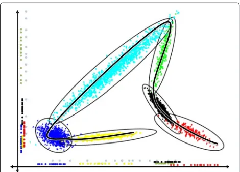
The concept of compactness from mathematical topol-ogy ([33], Chapter 3) states that a set, such as a manifold, can be covered by a finite number of open sets from theN-dimensional space.6There is no specific structure required for the covering sets, so they can be assumed to be Gaussian, i.e., ellipsoids. Figure 6 shows the cov-ering of a one-dimensional manifold (a curve) through a two-dimensional space. It can be seen that in order to use this approach the centers, orientations, and radii of the ellipsoids must be determined. Furthermore, any point on the manifold can be approximated arbitrarily well by this method simply by increasing the number of ellipsoids and also shrinking them to have a tighter fit. Statistically, hav-ing too many ellipsoids can cause undesirable overfitthav-ing effects, and mathematically, the number of ellipsoids (if it can be determined) is closely related to the manifold condition number.

The manifold-CS model described above is known in statistics as a mixture of factor analyzers (MFA). MFA combines the Gaussian mixture model (GMM) and fac-tor analysis. In MFA, the GMM determines the number of ellipsoids and the factor analyzer determines the statis-tics of each ellipsoid (location, orientation, and radii). Connecting the pixel omission example in Fig. 3 to the MFA is the final piece in CS-MFA. Figure 7 illus-trates the omission of dimensions of the measured data. The compressed data lies along the x- and y-axes. The CS inversion process—recovering the signal from com-pressed measurements—must take comcom-pressed measure-ments and map them back to the signal manifold. The model parameters learned by the MFA make this feasible by constraining the inversion procedure to the manifold.

One difficulty with the standard version of the GMM and factor analysis is that the number of clusters and

Fig. 7An illustration of the relationship between CS and MFA. The sensing matrix projects the new measured data along the axes. The measurements are missing a component and the job of CS inversion is to recover the missing component. In higher dimensions, the data is projected onto a subspace; several components are missing, and several components are available. In the experiments section, 4×4 patches are used and half of the pixels are blocked, so eight components are available and eight must be recovered for every patch. The CS inversion procedure maps the measurements back to the manifold using the previously learned MFA that approximates the manifold with ellipsoids

dimension of the basis must be set a priori. Cross-validation can be employed to determine the parameter settings, but it requires splitting the data into several sections and learning the model on each section. Bayesian nonparametrics [34] offers a solution to this problem by including these parameters in the inference of the model. The rest of this section will describe the mathematical details of the GMM, factor analysis, their nonparametric extensions, the MFA, and a description of the hardware needed for a TEM to collect data that can be inverted by CS-MFA.

Gaussian mixture model

The approach in this paper for manifold-CS is to model the manifold as an MFA. The mixture part of the MFA

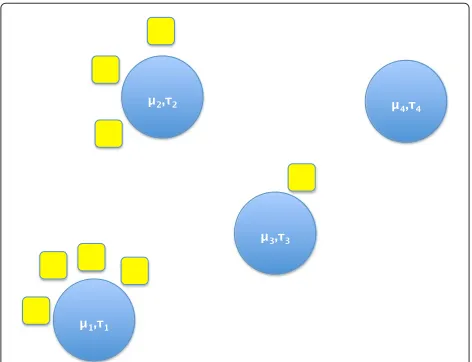
finds the number of ellipsoids needed to cover the man-ifold. The mixture part of MFA is based on the GMM, a model for clustering real-valued data. Figure 8 shows a set of two-dimensional data that was generated from a GMM. The primary goal in clustering is to determine which cluster each item belongs to and once this has been deter-mined, cluster statistics such as mean and variance can be determined. Meeting this primary goal is easily accom-plished by methods such asK-means. But the GMM goes beyond the primary goal by also finding the uncertainty parameters in the cluster assignments. In Fig. 8, several points lie in the overlap of two ellipses, withK-means they would simply be assigned to the nearest ellipse. In some applications, it may be important to know how strongly the algorithm believes a data point belongs to a cluster; this information can be inferred with the GMM.

The GMM is defined by the following hierarchical Bayesian model.7 _{In the GMM, the probability of a data} point given the means μ1,. . .,μT, precisions (inverse variances),τ1,. . . τT, and cluster weightsλ1,. . .,λT, is

p(xi|λ1,. . .,λT,μ1,. . .,μT,τ1,. . . τT)= T

t=1

λtN

μt,τt−1

,

(6)

whereT is the number of clusters andtis a specific clus-ter number. This says that the data point could lie in any of the clusters, so the probability is the sum over the prob-ability ofxibeing in each cluster. The rest of the hierarchy is defined as

xi|t(i)∼N

μt(i),τ_t−_(i1₎

(7)

μt∼N

a,b−1 (8)

τt∼G(c,d) (9)

λ1,. . .,λT ∼Dirichlet(α/T,. . .,α/T) (10) t(i)∼Multinomial(1;λ1,. . .,λT) (11)

where t(i) is the cluster number of the ith data point andG(·,·)is the gamma distribution, the conjugate prior for the precision of a normal distribution. The weight

λi determines the proportion of the data in clusteri. In Eq. (7), the cluster is known, so the probability is sim-ply defined by the statistics of that cluster. The mean and precision of each cluster are given by Eqs. (8)–(9). The hyperparameters a,b,c,d are usually determined using the mean and precision of the entire data set. The clus-ter proportions are sampled jointly from a symmetric Dirichlet distribution in Eq. (10). The Dirichlet distribu-tion is a multivariate extension of the beta distribudistribu-tion, where each λt ∈[ 0, 1] and Tt=1λt = 1. The param-eter α > 0 determines the decay rate of λ1,. . .,λT and will be discussed more below. Finally, the latent cluster assignments are drawn from a multinomial dis-tribution based on the cluster proportions. The multi-nomial distribution is a generalization of the Bernoulli distribution;n trials (data points) are performed with a chance of success in exactly one ofkdifferent categories (clusters).

A common method of inference in Bayesian modeling is Gibbs sampling, a Markov chain Monte Carlo (MCMC) method. In order to use Gibbs sampling, the probability of each model parameter must be able to be sampled given all the other parameters. Each parameter is sampled iter-atively until the model mixes; a model has mixed when the predicted distribution reaches a steady state. The sam-ples taken before the model mixes are called burn-in and are thrown away. Samples taken after the burn-in phase can be used to compute statistical approximations, which will be used later. For the cluster assignments, the probability of t(i) can be analytically averaged over all possibleλ1,. . .,λT. This is done by integrating the prod-uct of the distributions in Eqs. (10)–(11) with respect to

λ1,. . .,λT. The result is that the probability of a data item being assigned to a particular cluster is proportional to the number of data items already assigned to that cluster:

p(t(i)=j|t(−i),α)= n−ij+α/T

n−1+α , (12)

wheret(−i)is the list of all cluster assignments except the ith andn−ijis the number of items in clusterj, excluding itemi.

Returning to the number of clusters, it was previously mentioned that it is possible to infer the number of clus-ters using Bayesian nonparametrics. For the GMM, the nonparametric model is known as the infinite GMM and is produced by modifying the Dirichlet distribution to be a Dirichlet process (DP). There are a few analogies for the DP that have been well circulated in the statistics litera-ture, the Chinese restaurant process (CRP) and the stick breaking process (SBP). In this paper, the CRP and SBP, which are equivalent to the DP, will be introduced; the-oretical details of DP mixture models can be found in [17, 35, 36].

In the CRP, customers will choose a certain table with probability

p(occupied tablet)= nt n−1+α,

p(new table)= α

n−1+α, (13)

where n is the current number of customers,nt is the number of customers at table t, and α is the parame-ter related to the rate new tables are set up. To form a draw from a CRP, the infinity of customers are seated at their tables sequentially and after every customer has been seated the proportion of customers at each table deter-mines{λt}∞t=1. The CRP representation clearly shows the influence of α on the thickness of the tail of the pro-portions; increasing α increases the tail thickness. This countably infinite set of proportions replaces the finite number of proportions in the GMM. Informally, ifT → ∞in Eq. (12), then limiting cases are given by Eq. (13). Once the proportions have decayed past a certain level, the remaining proportions are set to zero and the num-ber of tables (clusters) can be determined. Figure 9 depicts the seating arrangement and assignment probabilities for a new customer after several customers have been seated. As previously mentioned, the primary function of the CRP is to draw an infinite set of random proportions. Another way to think of this is the SBP. In the SBP, a ran-dom proportion is drawn from Beta(1,α)and broken off a stick of unit length. Proportions are drawn from Beta(1,α) and broken from the remaining stick until the stick is gone (infinitely small). This approach achieves the same result

Fig. 9A depiction of the CRP after eight customers have been seated. The ninth customer will be seated at tables 1–3 with probabilities

4

as the CRP, but the SBP samples the proportions directly. Mathematically, the SBP is defined as

λt=vt t−1

j=1

(1−vj) (14)

vt∼Beta(1,α) (15)

and replaces Eq. (10) in the infinite GMM. As with the CRP, the SBP can be terminated when the proportions are sufficiently small. Figure 10 illustrates the stick breaking process.

Factor analysis

In the MFA approach to manifold-CS, a factor analyzer is used to determine the statistics of each ellipsoid cover-ing the manifold. Factor analysis is a statistical method for discovering a basis/frame for a dataset. The probabilistic model PCA [37], one of the most common types of factor analysis, is given in the following equations:

xi=Dwi+μ+i

dk∼N (0,P−1IP)

i∼N (0,γ−1IP)

(16)

where D =[d1|. . .|dK]∈ RN×K, μ ∈ RP is the mean offset,wi ∈ RK are Gaussian distributed weights,

i are Gaussian noise, and IN is the N × N identity matrix. In PCA, the data {xi}N_i=1 is used to discover

the matrix D whose column vectors span the space

of the data (up to noise) and wi are the transformed representations of xi. The algorithm has two parame-ters that need to be set K, the number of dictionary-elements/factors, and γ, the noise precision (inverse variance). The noise precision can also be modeled by a gamma random variable, so that it can also be inferred. Because thedk are Gaussian, the space

discov-ered is ellipsoidal. This can be seen through the following reparameterization:

xi∼N(μ,DD+γ−1IN). (17)

Using the singular value decomposition (SVD),DD =

K

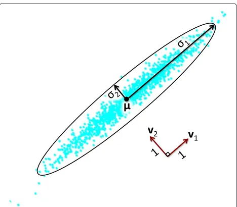
k=1σkvkv_k, where the singular vectorsvkare orthonor-mal and the singular valuesσk > 0. The singular values are the radii of a K-dimensional ellipsoid and the sin-gular vectors determine the orientation of each dimen-sion (assuming γ−1 < σK). Figure 11 illustrates the singular values and the mean. Note that probabilistic PCA is different from PCA, which is simply a projection onto the topKprincipal components (either via SVD of the data or eigen-decomposition of the data covariance matrix) [37].

As with the GMM, it is desirable to infer the number of dictionary elements necessary for the data. The solu-tion is again Bayesian nonparametrics. In factor analysis, the Beta-Bernoulli process (BeBP) is employed to infer the number of dictionary elements. The BeBP exhibits two additional features beyond the ability to infer the number of dictionary elements. First, the BeBP induces sparsity on the weights wi, and second, it allows infor-mation to be shared across the weights during infer-ence. The finite Beta-Bernoulli hierarchy is defined as follows

zki∼Bernoulli(πk), πk∼Beta a K,b

K−1 K

, (18)

whereKis the number of dictionary elements anda,bare hyperparameters. For eachxi∈RP, the latent binary vec-torzi ∈ RK encodes which dictionary elements are used by xi. The proportion πk is the sharing mechanism and encodes the average use of basis vectorkacross all of the selection vectorszi.

The metaphor used to describe the BeBP is the Indian Buffet Process (IBP). In the IBP, customers (data points) enter the restaurant and choose dishes (dictionary ele-ments) from the buffet. The first customer chooses Poisson(a) dishes. The ith customer samples each old dish with probability #(previous samples)/iand samples

Fig. 11An illustration of principal components analysis. The data points are described by anellipsecentered at the meanμof the data. The orientation of theellipseis determined by the principal vectors

v1,v2, and the radii are determined by principal valuesσ1,σ2. The

principal values also represent the distance of one standard deviation from the mean

Poisson(a/i)new dishes. This is the single parameter IBP withb=1. Figure 12 illustrates the process. As the num-ber of customersi tends to infinity, the number of new dishes tends to zero. In practice, the IBP is truncated to a number of dishes sufficiently large (i.e., large enough that some dishes are unused with high probability—this is data dependent) and any dishes that are unused can be removed from the representation. Details about the IBP and BeBP can be found in [17, 25].

Combining the BeBP with factor analysis results in the following beta process factor analysis [25]:

xi=Dwi+i (19)

dk ∼N (0,P−1IP) (20)

k ∼N (0,γ−1IP) (21)

γ∼G(c,d) (22)

wi=si◦zi (23)

si∼N (0,γs−1IK) (24)

γs∼G(e,f) (25)

zi∼ K

k=1

Bernoulli(π_k) (26)

π ∼ K

k=1

Beta a

K,b K−1

K

, (27)

where Eqs. (23)–(25) have replaced the expression for wi in the PCA model, ◦ is the element-wise Hadamard product, and the product notation in 26 and 27 denotes

independent draws. The mean μ has been omitted in

(19), since in the case of a single factor analyzer, the mean can simply be subtracted from the data as a pre-processing step. When implementing the algorithm, the hyper-parameters a,. . .,f are set to so-called non-informative values.

To make the connection to optimization approaches (e.g.,K-SVD), the negative log likelihood is

−logp(D,S,Z,π|X,a,b,c,d,e,f)

= γ

2 N

i=1

xi−D(si◦zi)22+ P 2

K

k=1

dk22

+ γs

2 N

i=1

si22

−logfBeta-Bern(Z;a,b)−log Gamma(γ|c,d)

−log Gamma(γs|e,f)+Const,

(28)

which is minimized to find the latent parameters. The first term is the least square error between the inferred parameters and the data while the second and third terms are commonly used as smoothing regularizers. The fourth term is the sparsifying regularizer, similar to the

1 norm. The BPFA model is commonly implemented

using Gibbs sampling or variational Bayesian methods [25, 30]. It must be emphasized that Eq. (28) is not used by sampling algorithms and cannot be optimized with traditional approaches. For more details about beta process dictionary learning including the application to three-dimensional data, see [38].

Mixture of factor analyzers

The MFA is realized by combining the GMM and the factor analyzer. The MFA is used to find an ellipsoidal cov-ering of the signal manifold. Equations (19) and (21) can be combined to create an equivalent representation (with the mean no longer omitted)

xi∼N

Dwi+μ,γ−1IN

. (29)

The new representation in Eq. (29) is the same format as the GMM. Now, the mixture of factor analyzers [30, 39, 40] can be introduced:

xi∼N

Dt(i)wi+μt(i),γ−,t1(i)IP

(30)

Dt(i)= ˜Dt(i)t(i) (31) ˜

d(_kt)∼N 0,P−1IP (32)

σ(t) kk ∼N

0,τ_tk−1

(33)

t(i)∼SBP(α) (34)

wi=si◦zt(i) (35)

si∼Nt(i)0,γ_s−1IK

(36) zt∼IBP(a,b) (37)

μt∼N

μ,τ₀−1IP

(38)

where γ,t,γs,t,τtk,τ0 all have gamma hyperpriors. Equation (30) says that data pointi is in a cluster with

statistics given by factor analyzer t(i). Equations (31)– (33) give a basis representation wheret(i)is a diagonal matrix similar to a singular value matrix that weights the contributions of each basis vector. If some of the (diagonal) elements of t are small relative to the noise variance, then that componentt(i)will be low rank.

The MFA is also a block-sparse model, concatenating all of the means and bases together

x=μ₁,D1|. . .|μT,DT ⎡ ⎢ ⎣ w1 .. . wT ⎤ ⎥ ⎦ (39)

where only one of the vectorswtis non-zero. In this way, only a single block or group is active, which also makes the representation sparse. If there is only a single ellipsoid in the model, then the sparse-CS formulation is recovered as a special case.

In addition to having a block-sparse structure, the non-parametric MFA usually infers bases that are low-rank, K < P. Low-rank Gaussian bases correspond to local-ized tubular manifolds. In [30] the fact that the signal is 1-block sparse is used to prove the reconstruction guar-antee. Theorems for the separability of the components and satisfaction of the restricted isometry property (RIP) can also be found in [30]. Essentially, the number of mea-surements should be greater than a constant times the largest rank among all of theDtplus the log of the number of components. The largest rank is the intrinsic manifold dimension, while the number of componentsTis related to the manifold condition number.

CS-MFA

In order to use the MFA for CS inversion, the proba-bility of the signal given the measurements needs to be determined,p(x|y), this requires the posterior predictive probabilityp(x)and the probability of the measurements given the signalp(y|x). The posterior predictive distribu-tion is the expected value of a new (predicted) data point with the expectation taken over the posterior

p(x)=

ˆ w

px| ˆwpwˆ|{xi}Ni=1,. . .

dwˆ

= ˆ w N

t=1

N x;D˜t(tdiag(zt))wˆ +μt,γ−,t1IP

N w;ˆ ξ_t,t

dwˆ

= T

t=1

λtN

x;χ_t, t

,

Fig. 13A schematic of the TEM setup for CACTI. After the beam passes through, the sample portions of it are occluded by the aperture. The occluded images are integrated together on the camera. Because each image has a different encoding, defined by the position of the aperture, they can be recovered by CS inversion. In order for each image to get a different encoding, the piezoelectric stage is driven by the function generator at a rate faster than the camera

where

χt= ˜Dt(tdiag(zt))ξt+μt (41)

t= ˜Dt(tdiag(zt))t(diag(zt)t)D˜t +γ−,t1IP. (42)

The prior predictive distribution is obtained whenξ_t =0 andt = IP, however this is usually inaccurate, so the posterior parameters are obtained by calculating the mean and covariance of the Gibbs samples. The basesD˜tare also taken as the mean of the Gibbs samples.

The probability of the measurements given the signal is also known

p(y|x)=N y;x,R−1, (43)

where R is the noise precision of the compressed noise

. By invoking Bayes’s rule, the order of the conditional

probability can be switched and after another reparame-terization, the desired probability is again a MFA.

p(x|y)= p(x)p(y|x) p(x)p(y|x)dx

= T

t=1

˜ λtN

x;χ˜_t, ˜t

, (44)

where

˜

λt= λt

N y;χ_t,R−1+ t

T

l=1λlN

y;χ_l,R−1+ l

(45)

˜ χt=

R+ −_t1

−1

(46)

˜_{t= ˜χtRy+} −1 t χt

. (47)

The representation in Eq. (44) admits an analytic CS inver-sion procedure, that is, once the model parameters are

learned (either offline or online [22, 41]), new signals are recovered by matrix–vector operations.

Description of CS-TEM hardware

The coding scheme, called pixel-wise flutter-shutter, blocks pixels on the camera while it is integrating. A single pixel of the measured image has the following representation:

Yij=

Aij1,Aij2,. . .,AijL

⎡ ⎢ ⎢ ⎢ ⎣

Xij1 Xij2 .. . XijL

⎤ ⎥ ⎥ ⎥

⎦ (48)

TheAijare binary indicators of whether pixelijis blocked in compressed frame, andXis the image. This represen-tation can be consolidated as

Yij=ijxij, (49)

and the completeis built by combining each pixel mask into a block diagonal matrix

=diag1,1,1,2,. . .,Nx,Ny

, (50)

where the image size isNx×Nypixels. As previously men-tioned, the images are broken down into patches so the data pointsxiin the MFA model are of size 4×4×L.

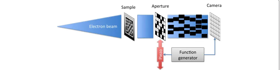
In order to obtain compressed measurements suitable for CS-MFA, the coded aperture compressive tempo-ral imaging (CACTI) approach described in [23, 42] is used. CACTI was developed for optical video CS. In the CACTI camera system, the signal passes through a coded aperture that changes at a faster rate than the camera obtains images. This causes multiple coded images to be integrated into a single image. The aperture is set on a piezoelectric stage. The stage moves along either thex- or y-axis according to a triangle wave. During an up-stroke, a set of coded images are integrated and then another set are integrated during the down-stroke. A function gener-ator is used to drive the piezo stage and trigger the image capture on the camera at the troughs and peaks of the tri-angle wave. The same setup is possible in TEM. The major difficulty in moving this approach to TEM is designing an aperture to block electrons rather than photons. Figure 13 shows an illustration of the TEM-CACTI system.

The benefit of placing the mask on a moving stage is that moving the mask creates a new encoding—essentially a new mask. If the position of the mask is known, then the encoding is known. This overcomes a difficulty in CS of using a new mask for every measurement. The com-pression ratio is determined by the range of motion of the mask. Effectively, movingnpixels (mask feature size) will give a factor ofncompression, ornframes from 1.

Another difficulty—present in CS for TEM, but not in optical CS—is that the part of the mask blocking the signal must be supported by a material transparent to electrons.

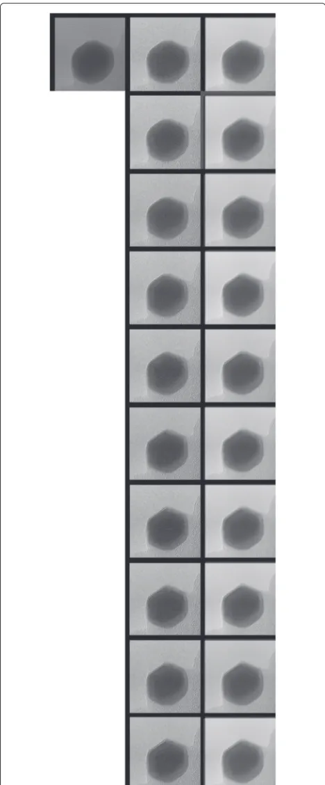
Fig. 15An illustration of CS inversion from 10 frames compressed into 1. Thetop leftimage shows the compressed frame, themiddle

columnof images shows the reconstructed frames, and theright

columnshows the original frames. During the sequence, a peak atop

Example masks that allow approximately 50 % of elec-trons to pass are shown in Fig. 14. An issue that might be raised about this approach is that 50 % of the image is dis-carded. The intent of our approach, however, is to increase the acquisition rate. It has been shown that image data can be discarded and subsequently recovered, both gen-erally [25] and in electron microscopy [13]. Moreover, it might be possible to place the aperture before the speci-men, which would give a decrease in dose and an increase in acquisition rate.

Results and discussion

The results in this section show the efficacy of the CS approach to TEM video. First, the algorithm settings and simplifications are given. Second, two example videos are discussed. Third, the relationship between the com-pression ratio and reconstruction quality is shown to be approximately logarithmic. The reconstruction qual-ity decreases more slowly as the compression factor increases. The standard deviation of the average PSNR is also well-behaved. The simulation used real TEM video and sampled it according to the CACTI scheme. The CS reconstruction is then compared against the original for a quantitative error analysis. The images are the direct out-put of the CS algorithm and havenotbeen post processed. Note:The images are best viewed digitally and full image resolution is available via the zoom function in most PDF readers.

Sampling approaches are computationally expensive (and usually scale poorly with respect to the data size), so we relax the factor analysis constraint and simply use a (finite) GMM. The GMM can be fit very efficiently by expectation-maximization ([19], chapter 9). The develop-ment above shows that this simplification is well-founded and the results below show that the simplification still pro-duces adequate results. For training the GMM, we use the algorithm supplied by the MATLAB statistics tool-box with T = 20 and regularization parameter 10−8. The only other parameters are the patch size and patch spacing.

For all three experiments, the patch size was 4×4×2, and these were extracted half-overlapping (the spacing between the patches was 2× 2 × 1). In the first two experiments, the compression factor was 10 frames, so the rate is 10 to 1. To train the GMM model, the first few frames were used, specifically frames 1, 4, 7,. . ., 3N+1, whereN is the number of frames compressed in 1 mea-surement. Training the GMM model on other data also works well (and is more practical), but those results are not reported here. The reconstruction also proceeded by shifting 5 frames at a time (or half of the compression ratio in the last experiment). This adds temporal stability by averaging nearby reconstructions. The silver nanoparticle video has over 900 frames each with 1024×1024 pixels, or roughly 235 million half-overlapping patches that were reconstructed in a few hours on a workstation.

Palladium nanoparticle oxidation

To demonstrate the applicability of coded aperture CS video reconstruction for atomic resolution imaging, we show observations from Pd nanoparticles during expo-sure to elevated temperature and an oxidizing environ-ment. Supported Pd nanoparticles are used extensively in catalytic applications under high temperatures and in reactive gas environments. The ability to visualize and characterize morphological, structural, and surface transformations associated with environmental exposure under in-situ conditions at high temporal resolution is critical for rationalization of structure–property relation-ships and thus essential for future advancement of cat-alytic technologies.

The observations here focus on characterization of atomic level processes associated with a formation of a surface oxide in the initial stage of oxidation. In particu-lar, the observations show how adsorption of oxygen and interaction with a SiNxsupport lead to subtle morpholog-ical changes, and subsequently to a formation of surface oxides. The observations were performed with an envi-ronmental FEI Titan 80–300. The microscope is equipped with CEOS aberration corrector for the image-forming

Fig. 17This figure is a plot of the PSNR for each reconstructed frame in the 10×compressed palladium nanoparticle video. At the beginning, the PSNR is low because of the top and left edge missing in the reconstruction, this is due to the coded aperture. Many frames are reconstructed with a translational component, for example, frame 134. After registration, these frames have a reconstruction PSNR similar to the average

lens, which allows imaging with Ångström resolution. The images were acquired with Gatan’s Ultra-Scan 1000S CCD camera, and the acquisition was performed in Dig-ital Micrograph (DM) at the frame rate of 1.1 frames/s. The observations were performed at oxygen partial pres-sure of 10−2mbar at 500 °C. Heating of the samples was done with an Aduro Protochips heating holder.

From the originally recorded video of Pd oxidation, which is available in the supplementary information, CS video reconstruction was simulated by integrating every 10 aperture-coded frames into a single measurement frame. A subset of 10 original images, the integrated coded image, and reconstructed images are shown in Fig. 15. The comparison in Fig. 15 shows very good agreement between the original and reconstructed images. Figure 16 shows the last frame recovered from a set of compressed frames—the peaked feature is accurately recovered. The

reconstruction preserves the atomic resolution in the bulk portion of the nanoparticles with a small loss of resolu-tion observed in the interfacial region. The peak signal to noise ratio (PSNR) for each recovered frame is shown in Fig. 17. The large drop in PSNR is due to misalign-ment, and after registering the reconstructed image with the original, the PSNR is 16.95 dB. The reason for the relatively low PSNR overall (despite the fact that the reconstructionlooksgood, Fig. 18) is due to the fact that the reconstructed image is denoised as a side effect of reconstruction. Moreover, the top and left edges of the image (10 pixels) are mostly lost due to the coding process.

Silver nanoparticle coalescence

Using aberration-corrected environmental TEM, hetero-geneous catalysts surface restructuration by gas molecules [43], the sintering mechanisms of supported metal cat-alysts [44], and other structural changes in a gaseous environment [45], can be studied at the atomic scale under gas pressures of up to 20 Torr. For gas pressures closer to catalytic conditions, up to 1 Atm, subnanometer resolution can be achieved by using dedicated gas cell holders [46, 47]. In order to gain in-situinformation at the atomic level, highly magnified imaging is required. Typically, an increase in magnification results in the elec-tron beam having to be focused onto a smaller area in order to keep the number of electrons per pixel constant. This increase in the electron dose will ultimately lead to an increase of possible beam damage effects that can influence the process. Here we show an example of metal-lic particle coalescence induced merely by parallel elec-tron beam illumination in TEM. While our experiments have been done for 60 nm Ag particles, we expect addi-tional or more pronounced beam effects for the case of smaller particles. This is most relevant for catalysis appli-cations, since particle mobility during sintering will be higher.

Figure 19 shows a sequence of bright field TEM images of the electron beam-induced coalescence of six Ag nanoparticles supported on amorphous carbon. Commer-cially available 60-nm-diameter Ag particles (0.02 mg/mL

Fig. 19A sample of frames from the Ag particle video. The video shows the electron beam-induced coalescence of six Ag nanoparticles. These images have been cropped to show only the Ag nanoparticles

in aqueous buffer, Sigma-Aldrich) were drop cast on a holey carbon film (Ted Pella, Inc.). As with the previ-ous example, thein-situTEM videos were acquired using an 80–300 keV FEI Titan environmental TEM equipped with an objective-lens spherical aberration corrector and

operating at 300 keV and in high vacuum mode. Changes in image contrast are observed, indicating particular dynamic processes, such as the formation of cavities, localized areas with lighter contrast within the particles and adjacent to areas displaying surface expansion, and

diffraction contrast due to recrystallization, apparent as broad linear contours. Mass transport is apparent as pro-gressive changes in contrast from the darker particles to the lighter inter-particles and the surface of newly formed areas. After about 10 min of electron-beam irradiation, a recrystallization front is formed and advances from the top left corner of the forming crystal down. After 13 min of irradiation, formation of facets on the recrystallized surface is also observed. The mass transport during irra-diation, as shown in the snapshots for the first 2 min of the process, occurs first at the sintering neck between particles and homogeneously around their surfaces on the outermost particles. This indicates that surface diffu-sion is a main mechanism driving the coalescence process under the electron beam. This observation is in good agreement with previous works [48, 49].

A set of reconstructed frames are shown for comparison in Fig. 20. The images in Fig. 20 are qualitatively accu-rate when compared to Fig. 19. In the last 200 frames, the specimen begins to drift up and left. The reconstruction quality diminishes during this phase, as shown by Fig. 21, since the training data did not include drift dynamics. Of note, however, is a bright flash that occurs near frame 850, the reconstruction completely eliminates this transient effect (the image became mostly white in a few frames and then returned to the original contrast over the same period). Moreover, the speckled noise is also removed— it is especially apparent in the background of the original data. The reconstruction PSNR of the Ag nanoparticle experiment is relatively higher than the PSNR of Pd recon-struction because the noise in the original Ag data is much lower.

Fig. 21This figure shows the PSNR over time of the Ag nanoparticle video. The reconstruction quality is very good until the last 200 frames when the specimen drifts up and left. This kind of motion was not incorporated into the model, which explains why the reconstruction quality suffers in this portion of the video

Fig. 22The average PSNR (dB) is plotted over a range of compression factors for CS-MFA and linear interpolation for the palladium nanoparticle video. Theerror barscorrespond to 1 standard deviation. Best fit logarithmic curves are also displayed

Compression versus reconstruction quality

The final experiment compares the reconstruction quality over several compression levels. Figures 22 and 23 show the average PSNR across all video frames as a function of the compression factor. These curves are approxi-mately logarithmic. As the compression factor increases, the average PSNR decreases more slowly. This kind of saturation occurs because the reconstructed image is increasingly smooth, but still maintains the average image, thus it cannot have a very low PSNR.

For comparison, the average PSNR of linear interpola-tion is also plotted. This is simply a baseline, it would be difficult to do worse with a principled approach. For example, when the video has been subsampled with compression factor 2 (i.e., every other frame is missing), the interpolated result is the average of the previous frame and the next frame. The compressed video used for the interpolation results is simply subsampled at the rate cor-responding to the compression factor. To compute the average PSNR, all of the sampled frames are omitted, since their PSNR is infinite. Therefore, the comparison is between the inferred frames of both methods.

The comparison between CS-MFA and interpolation shows that the compressed frames contain significant information. CS-MFA is able to exploit this information to achieve accurate results for a wide range of compression

factors. Moreover, the variance in the reconstruction PSNR is relatively small and does not increase with the compression factor.

Finally, reconstructed frames from both movies at 10×, 20×, and 30× compression can be seen alongside the original frames in Figs. 24 and 25. As the compression level increases, the image contrast decays. Many of the important structures are still visible in reconstructed images, and the reconstructed images are denoised. The edge artifacts in the palladium video are from an image alignment that occurred prior to the CS simulation.

It is difficult to decide from Figs. 22 to 23 what the max-imum compression factor should be. The reconstructed images degrade very smoothly. Upon inspection of the reconstructed videos (included in the supplementary material), a compression of about 15×seems feasible for

Fig. 25Fromtoptobottomoriginal, 10×, 20×, and 30×compressed reconstruction; fromlefttorightframes 113, 349, and 733. Again, a significant denoising effect can be seen in the reconstructed images. The salient features remain, but contrast reduces as compression increases. The structure in thebottom leftof the original frame 733 has disappeared from the reconstructions, this is likely because nothing like the structure existed in the training data

the palladium nanoparticle video and about 20×for the silver nanoparticle video. The compression factor also depends on what image features are important; this is a tradeoff between speed and image clarity.

Conclusions

In this paper, we have provided an overview of CS and CS recovery via MFA. By using real TEM data to simulate the effects of compression, we were able to show the feasibility of video CS for TEM. The videos that were recovered from the simulated CS measurements exhibit the salient features of the material dynamics being stud-ied at a compression factor of 10–20×. Balancing the information required, the signal to noise of the image and the desired resolution suggests that the compression

could be increased even further for other experiments— dramatically improving the temporal resolution of obser-vations in the TEM. Work to build a prototype aperture to collect compressively sensed video is currently underway. If successful, such an approach will be able to improve the ability to observe materials dynamics in any TEM imaging system.

Endnotes

1_{AnN-dimensional basis can be formed by taking the}

Kronecker product ofNcopies of the 1-dimensional basis.

2_{The sensing scheme must satisfy the restricted}

3_{The form used in equation (1) is built by stacking all of}

thexi,yiinto single vectors and placing theiinto a block diagonal matrix.

4_{Frames are a generalization of bases. A frame can have}

a different number of elements than a basis. If the dimension of the space isN, then a basis will haveN elements of dimensionN, whereas a frame will have K=Nelements of dimensionN. WhenK>Nthe frame is sometimes referred to as an “overcomplete basis”.

5_{If the dictionary is inR}N×K_{,K>N, the number of}

dictionary elements used is much smaller thanK. The actual number of elements used depends on the compressibility of the signal.

6_{More formally, if{A}

i}is an open cover of a setSin a metric space, thenSis compact if

S⊂Ai1∪Ai2∪. . .Ain,

where the number of indicesnis finite.

7_{The one-dimensional version is presented for}

simplicity and is easily generalized with the Wishart distribution.

Competing interests

This work was funded through projects at Pacific Northwest National Laboratory (PNNL). The indicated authors receive salary from their respective institutions. PNNL will pay for publishing fees. We are in the process of patenting this work.

Authors’ contributions

AS wrote the bulk of the manuscript, helped determine the approach for using the prescribed algorithm on TEM video, performed the compressive reconstructions, and conducted the numerical experiment comparing compression ratios. LK performed the palladium nanoparticle experiment and wrote that section of the paper, likewise for PA for the silver nanoparticles, LK also edited the manuscript. XY devised and implemented the algorithm and helped determine the best approach for applying it to TEM video. LC also worked on the development of the algorithm. NDB determined appropriate experiments to demonstrate the method, wrote the introduction, and was the primary editor of the manuscript. All authors read and approved the final manuscript.

Acknowledgements

This work was supported in part by the United States Department of Energy Grant No. DE-FG02-03ER46057. This research is also part of the Chemical Imaging Initiative conducted under the Laboratory Directed Research and Development Program at Pacific Northwest National Laboratory (PNNL) and was performed using EMSL, a national scientific user facility sponsored by the Department of Energy’s Office of Biological and Environmental Research located at PNNL. PNNL is a multi-program national laboratory operated by Battelle Memorial Institute under Contract DE-AC05-76RL01830 for the U.S. Department of Energy.

Received: 11 June 2015 Accepted: 11 June 2015

References

1. Ferreira, PJ, Mitsuishi, K, Stach, EA:In-situtransmission electron microscopy. MRS Bull.33, 83–90 (2008)

2. Jinschek, JR: Advances in the environmental transmission electron microscope (etem) for nanoscalein-situstudies of gas-solid interactions. Chem. Commun.50, 2696–2706 (2014)

3. Huang, JY, Zhong, L, Wang, CM, Sullivan, JP, Xu, W, Zhang, LQ, Mao, SX, Hudak, NS, Liu, XH, Subramanian, A, Fan, H, Qi, L, Kushima, A, Li, J:In-situ

observation of the electrochemical lithiation of a single SnO2nanowire electrode. Science.330(6010), 1515–1520 (2010)

4. Evans, JE, Jungjohann, KL, Browning, ND, Arslan, I: Controlled growth of nanoparticles from solution within-situliquid transmission electron microscopy. Nano Lett.11(7), 2809–2813 (2011)

5. Krivanek, OL, Dellby, N, Lupini, AR: Towards sub-Å electron beams. Ultramicroscopy.78(14), 1–11 (1999)

6. Haider, M, Rose, H, Uhlemann, S, Kabius, B, Urban, K: Towards 0.1 nm resolution with the first spherically corrected transmission electron microscope. J Electron. Microsc. (Tokyo).47(5), 395–405 (1998) 7. Jinschek, JR, Helveg, S: Image resolution and sensitivity in an

environmental transmission electron microscope. Micron.43(11), 1156–1168 (2012)

8. Gatan: TEM Imaging & Spectroscopy. http://www.gatan.com/products/ tem-imaging-spectroscopy. Accessed: 19 Dec 2014

9. McMullan, G, Faruqi, AR, Clare, D, Henderson, R: Comparison of optimal performance at 300 kev of three direct electron detectors for use in low dose electron microscopy. Ultramicroscopy.147, 156–163 (2014) 10. Candès, EJ, Romberg, J, Tao, T: Uncertainty principles: exact signal

reconstruction from highly incomplete frequency information. Inform. Theory IEEE Trans.52(2), 489–509 (2006)

11. Donoho, DL: Compressed sensing. Inform. Theory IEEE Trans.52(4), 1289–1306 (2006)

12. Binev, P, Dahmen, W, DeVore, R, Lamby, P, Savu, D, Sharpley, R: Compressed sensing and electron microscopy. In: Vogt, T, Dahmen, W, Binev, P (eds.) Modeling Nanoscale Imaging in Electron Microscopy. Nanostructure Science and Technology, pp. 73–126. Springer, (2012) 13. Stevens, A, Yang, H, Carin, L, Arslan, I, Browning, ND: The potential for Bayesian compressive sensing to significantly reduce electron dose in high-resolution STEM images. Microscopy.63(1), 41–51 (2013) 14. Liao, X, Li, H, Carin, L: Generalized alternating projection for weighted-2,1

minimization with applications to model-based compressive sensing. SIAM J. Imaging Sci.7(2), 797–823 (2014)

15. Bioucas-Dias, JM, Figueiredo, MA. T: A new TwIST: Two-step iterative shrinkage/thresholding algorithms for image restoration. Image Process. IEEE Trans.16(12), 2992–3004 (2007)

16. Mairal, J, Bach, F, Ponce, J: Sparse modeling for image and vision processing (2014). arXiv preprint arXiv:1411.3230

17. Griffiths, T, Ghahramani, Z: The Indian buffet process: an introduction and review. J. Mach. Learn. Res.12, 1185–1224 (2011)

18. Baraniuk, RG: Compressive sensing. IEEE Signal Process. Mag.24(4) (2007) 19. Bishop, CM,et al: Pattern Recognition and Machine Learning. Springer,

New York (2006)

20. Foucart, S, Rauhut, H: A Mathematical Introduction to Compressive Sensing, Springer, New York (2013)

21. Gill, J: Bayesian Methods: A Social and Behavioral Sciences Approach. CRC press (2014)

22. Yuan, X, Yang, J, Llull, P, Liao, X, Sapiro, G, Brady, DJ, Carin, L: Adaptive temporal compressive sensing for video. In: Image Processing (ICIP), 2013 20th IEEE International Conference On, pp. 14–18, Melbourne, Australia, (2013)

23. Yuan, X, Llull, P, Liao, X, Yang, J, Brady, D, Sapiro, G, Carin, L: Low-cost compressive sensing for color video and depth. In: Computer Vision and Pattern Recognition (CVPR), 2014 IEEE Conference On. IEEE, (2014). arXiv:1402.6932v1

24. Saghi, Z, Benning, M, Leary, R, Macias-Montero, M, Borras, A, Midgley, PA: Reduced-dose and high-speed acquisition strategies for

multi-dimensional electron microscopy. Adv. Struct. Chem. Imaging (2015)

25. Zhou, M, Chen, H, Paisley, J, Ren, L, Li, L, Xing, Z, Dunson, D, Sapiro, G, Carin, L: Nonparametric Bayesian dictionary learning for analysis of noisy and incomplete images. Image Process. IEEE Trans.21(1), 130–144 (2012) 26. Olshausen, B,et al: Emergence of simple-cell receptive field properties by

learning a sparse code for natural images. Nature.381(6583), 607–609 (1996)

28. Binev, P, Blanco-Silva, F, Blom, D, Dahmen, W, Lamby, P, Sharpley, R, Vogt, T: High-quality image formation by nonlocal means applied to high-angle annular dark-field scanning transmission electron microscopy

(HAADF–STEM). In: Vogt, T, Dahmen, W, Binev, P (eds.) Modeling Nanoscale Imaging in Electron Microscopy. Nanostructure Science and Technology, pp. 127–145. Springer, (2012)

29. Goris, B, den Broek, WV, Batenburg, KJ, Mezerji, HH, Bals, S: Electron tomography based on a total variation minimization reconstruction technique. Ultramicroscopy.113, 120–130 (2012)

30. Chen, M, Silva, J, Paisley, J, Wang, C, Dunson, D, Carin, L: Compressive sensing on manifolds using a nonparametric mixture of factor analyzers: algorithm and performance bounds. Signal Process. IEEE Trans.58(12), 6140–6155 (2010)

31. Wakin, MB: Manifold-based signal recovery and parameter estimation from compressive measurements (2010). arXiv preprint arXiv:1002.1247 32. He, X, Yan, S, Hu, Y, Niyogi, P, Zhang, H-J: Face recognition using

laplacianfaces. Pattern Anal. Mach. Intell. IEEE Trans.27(3), 328–340 (2005) 33. Munkres, JR: Topology: A First Course. Prentice-Hall Englewood Cliffs, NJ

(1975)

34. Gershman, SJ, Blei, DM: A tutorial on Bayesian nonparametric models. J. Math. Psychol.56(1), 1–12 (2012)

35. Rasmussen, C: The infinite Gaussian mixture model. In: NIPS, pp. 554–560, Denver, CO, (1999)

36. Neal, RM: Markov chain sampling methods for Dirichlet process mixture models. J. Comput. Graph. Stat.9(2), 249–265 (2000)

37. Tipping, ME, Bishop, CM: Probabilistic principal component analysis. J. R. Stat. Soc. Series B (Stat. Methodol.)61(3), 611–622 (1999) 38. Xing, Z, Zhou, M, Castrodad, A, Sapiro, G, Carin, L: Dictionary learning for

noisy and incomplete hyperspectral images. SIAM J. Imaging Sci.5(1), 33–56 (2012)

39. Ghahramani, Z, Hinton, GE,et al: The EM algorithm for mixtures of factor analyzers (1996). Technical report, Technical Report CRG-TR-96-1, University of Toronto

40. Tipping, M, Bishop, C: Mixtures of probabilistic principal component analyzers. Neural Comput.11(2), 443–482 (1999)

41. Yang, J, Yuan, X, Liao, X, Llull, P, Sapiro, G, Brady, DJ, Carin, L: Gaussian mixture model for video compressive sensing. In: Image Processing (ICIP), 2013 20th IEEE International Conference On, pp. 19–23, (2013)

42. Llull, P, Liao, X, Yuan, X, Yang, J, Kittle, D, Carin, L, Sapiro, G, Brady, D: Coded aperture compressive temporal imaging. Opt. Express.21(9), 10526–10545 (2013)

43. Yoshida, H, Kuwauchi, Y, Jinschek, JR, Sun, K, Tanaka, S, Kohyama, M, Shimada, S, Haruta, M, Takeda, S: Visualizing gas molecules interacting with supported nanoparticulate catalysts at reaction conditions. Science. 335(6066), 317–319 (2012)

44. DeLaRiva, AT, Hansen, TW, Challa, SR, Datye, AK:In-situtransmission electron microscopy of catalyst sintering. J. Catalysis.308, 291–305 (2013) 45. Jinschek, J: Advances in the environmental transmission electron

microscope (ETEM) for nanoscalein-situstudies of gas-solid interactions. Chem. Commun.50(21), 2696–2706 (2014)

46. Creemer, J, Helveg, S, Hoveling, G, Ullmann, S, Molenbroek, A, Sarro, P, Zandbergen, H: Atomic-scale electron microscopy at ambient pressure. Ultramicroscopy.108(9), 993–998 (2008)

47. Mehraeen, S, McKeown, JT, Deshmukh, PV, Evans, JE, Abellan, P, Xu, P, Reed, BW, Taheri, ML, Fischione, PE, Browning, ND: A (S)TEM gas cell holder with localized laser heating forin-situexperiments. Microscopy Microanal.19(02), 470–478 (2013)

48. Tsyganov, S, Kästner, J, Rellinghaus, B, Kauffeldt, T, Westerhoff, F, Wolf, D: Analysis of Ni nanoparticle gas phase sintering. Phys. Rev. B.75(4), 045421 (2007)

49. Surrey, A, Pohl, D, Schultz, L, Rellinghaus, B: Quantitative measurement of the surface self-diffusion on Au nanoparticles by aberration-corrected transmission electron microscopy. Nano Lett.12(12), 6071–6077 (2012) 50. Candès, EJ: The restricted isometry property and its implications for

compressed sensing. Comptes Rendus Mathematique.346(9), 589–592 (2008)

Submit your manuscript to a

journal and benefi t from:

7Convenient online submission 7Rigorous peer review

7Immediate publication on acceptance 7Open access: articles freely available online 7High visibility within the fi eld

7Retaining the copyright to your article