Analyzing airﬂow in static ice caves by using the calcFLOW method

(1)

www.the-cryosphere.net/10/879/2016/ doi:10.5194/tc-10-879-2016

Analyzing airflow in static ice caves by using the calcFLOW method

Christiane Meyer1, Ulrich Meyer2, Andreas Pflitsch3, and Valter Maggi1

1_{Universita di Milano-Bicocca, Dipartimento di Scienze Ambiente e Territorio e Scienze della Terra, Piazza della Scienza 1,} 20126 Milan, Italy

2_{University of Bern, Astronomical Institute, Sidlerstrasse 5, 3012 Bern, Switzerland}

3_{Ruhr-University Bochum, Geography Department, Working Group Cave- and Subway-Climatology, Universitätsstrasse} 150/Building NA, 44780 Bochum, Germany

Correspondence to: C. Meyer ([email protected])

Received: 29 July 2015 – Published in The Cryosphere Discuss.: 30 September 2015 Revised: 29 March 2016 – Accepted: 13 April 2016 – Published: 25 April 2016

Abstract. In this paper we present a method to detect airflow through ice caves and to quantify the corresponding airflow speeds by the use of temperature loggers. The time series of temperature observations at different loggers are cross-correlated. The time shift of best correlation corresponds to the travel time of the air and is used to derive the airflow speed between the loggers. We apply the method to test data observed inside Schellenberger Eishöhle (ice cave). The suc-cessful determination of airflow speeds depends on the exis-tence of distinct temperature variations during the time span of interest. Moreover the airflow speed is assumed to be con-stant during the period used for the correlation analysis. Both requirements limit the applicability of the correlation analy-sis to determine instantaneous airflow speeds. Nevertheless the method is very helpful to characterize the general pat-terns of air movement and their slow temporal variations. The correlation analysis assumes a linear dependency be-tween the correlated data. The good correlation we found for our test data confirms this assumption. We therefore in a second step estimate temperature biases and scale factors for the observed temperature variations by a least-squares adjust-ment. The observed phenomena, a warming and an attenua-tion of temperature variaattenua-tions, depending on the distance the air traveled inside the cave, are explained by a mixing of the inflowing air with the air inside the cave. Furthermore we test the significance of the determined parameters by a standard

F test and study the sensitivity of the procedure to common manipulations of the original observations like smoothing. In the end we will give an outlook on possible applications and further development of this method.

1 Introduction

(2)

analy-sis. Besides financial reasons, ice cave studies are facing two other problems in general: the accessibility of the study site and the energy supply for technical devices. The study sites are in many cases in remote places in the high mountains, ex-posed to avalanches and winter conditions often lasting sev-eral months. As a consequence, e.g., airflow measurements using sonic anemometers are not always possible, though an understanding of the airflow regime is indispensable for the understanding of these complex systems (e.g., Pflitsch and Piasecki, 2003). For the development but also degradation of subterranean ice, the airflow regime is the main influencing factor beside the time/amount of water and the thermal con-ditions or the heat transfer between the different media (rock, ice, water, air) (Korzystka et al., 2011). Racovitza (1927) states that the main factor that characterizes a cave in general is the air temperature. Among the deduced topoclimatologi-cal factors, the airflow regime, which is first of all determined by the thermal relation between the exterior atmosphere and the cave atmosphere, is the most important physical fac-tor to describe the topoclimate of a cave. For this reason Racovitza (1975) proposes to classify the different types of cave topoclimate using the diverse types of airflow regimes. Lütscher and Jeannin (2004a) propose, for the specific case of ice caves in temperate regions, to classify on the basis of two criteria: cave air dynamics and the type of ice. They explain this by the importance of the airflow regime as the “dominating process at the origin of cave ice” in, e.g., static or dynamic ice caves, just to mention the best known ice cave types. Numerous case studies highlight the role of air-flow for the development of ice caves, (e.g., Lütscher and Jeannin, 2004b; Pflitsch et al., 2007; Morad et al., 2010). For these reasons we present here calcFLOW, a practical at-tempt to use the database which is available for the majority of ice caves, i.e., air temperature measurements for comput-ing air fluxes. In this paper we present the basic principles and the methodology of the calcFLOW method and apply it to Schellenberger Eishöhle (Germany). The results allow the interpretation of observations that have so far not been well understood, but also reveal principle shortcomings of the setup of the loggers that limit the analysis. They will be useful to install a refined network of temperature loggers inside the cave. We are convinced that also other observa-tion campaigns may benefit from analysis by the calcFLOW method. In the last part of this paper possible further appli-cations of the calcFLOW method are discussed. All calcula-tions were conducted by using the GNU Octave open-source software1.

2 Study site and data

Bögli (1978) defined ice caves as caves containing ice all year around. One can further distinguish different types

1_{https://www.gnu.org/software/octave/}

based on the origin of the ice, the main ice building pro-cesses, and the type of the ventilation (Lütscher, 2005). Ice caves occur mainly at elevations below the 0◦_{C isotherm}

(in the Alps at about 2000 m elevation) due to the availabil-ity of water, but they may also occur in permafrost regions (Lütscher and Jeannin, 2002). Boundary criteria, which ad-ditionally limit the existence of ice caves are the airflow sys-tem, the number of surface openings, and the cave morphol-ogy. One common type are the static ice caves. Like in our example, this kind of ice cave only has one natural entrance, which is situated in the upper or middle part of the cave, and therefore acts like a cold air trap. In summer, when outside temperatures are above the cave air temperatures, the cooler air stays in the cold air trap and is only slowly warmed by the surrounding rock. Stable temperature stratification oc-curs when deep temperatures are preserved over summer. The open phase or so-called “winter situation”, when air change with the external atmosphere occurs, is limited to ex-ternal temperatures below the cave air temperatures. When outside temperatures drop below the current cave air temper-ature, the colder air replaces the warm air inside the cave. The cold air enters the cave along the floor of the cave passages, while the warm air is pushed out along the ceiling towards the cave entrance. The temperatures observed close to the cave floor and at the ceiling therefore may differ greatly. For this reason care has to be taken in the selection of the positions for the temperature loggers to capture the airflow of interest. By the mixing of cold and warm airflows and by the contact of the inflowing cold air with the cave walls and cave ice, the inflowing air will gradually warm up, and on the other hand, the cave is cooled down from the entrance towards its inner reaches. As a consequence the stratification of the cave air is disturbed. Instead, the air temperature positively correlates with the distance the air traveled inside the cave. Temper-atures recorded along the floor of descending passages that track the inflowing cold air will show an inverted gradient compared to temperatures observed during the closed phase. As soon as the outside temperatures rise above the cave tem-perature and the inflow of cold air stops the stratification of the air is restored.

(3)

Figure 1. Location of Schellenberger Eishöhle at the foot of the east face of Untersberg. The mountain is viewed from the East, the

AG and DI Wenger-Oehn, digital elevation model: Bundesamt für Eich- und Vermessungswesen in Wien). The map inlay shows the location of Untersberg in Germany.

Josef-Ritter-von-Angermayer-Halle, the largest room in the cave with a length of 70 m and a width of 40 m, that is il-luminated by daylight. The floor of this hall, 17 m below the entrance level, completely consists of a major ice mono-lith, which is surrounded by the cave trail. The two passages Wasserstelle and Mörkdom connect to the deepest part of the ice cave called Fuggerhalle, 41 m below entrance level. They are also partly covered with ice. Temperature loggers were placed in Angermayerhalle (T1 and T4), along one of the passages leading downwards (Wasserstelle: T2), and in Fug-gerhalle (T3, see Fig. 2). The loggers recorded temperature data with an interval of 10 resp. 15 min. These temperature measurements were recorded for a first cave climate study of Schellenberger ice cave (compare Meyer et al., 2014; Grebe et al., 2008) and the logger setup was not optimized for the application of the calcFLOW method. Therefore synchroniz-ing the samplsynchroniz-ing rates of the different loggers was not em-phasized. Analyzing the observed temperature data, several questions arose. The two loggers in Angermayerhalle show quite different temperature behavior that could not easily be explained. Moreover the logger in Fuggerhalle recorded tem-peratures that seemed to be too warm for the lowest part of the ice cave where the coldest air was expected. The devel-opment of the calcFLOW method was motivated by these observations and led to reasonable explanations for the ob-served phenomena.

3 The model

As described in Sect. 2, two different stages of a static ice cave have to be distinguished: an open and a closed phase.

Fuggerhalle

Wasserstelle Mörkdom* Schellenberger ice cave ice part- ground view Based on the survey of Fritz Eigert 1959 drawing: F. Seewald

digitization: Christiane Meyer

Air temperature

measurements Angermayerhalle

lower part

Angermayerhalle upper part T4

T1 T2

T3

* No data for the example epoch of our calculation. Entra

nce

Estimated ice extent

0 m 25 m

Entrance

Angermayerhalle lower part

Fuggerhalle

Schellenberger ice cave

Schematic illustration of the side view

Angermayerhalle upper part

Wasserstelle Mörkdom

Direction to the

deeper non-ice part of the cave

Measuring point Unknown extent of ice

snow cone

Ice Snow + 50 m

0 m - 50 m - 100 m - 150 m - 200 m Side view -view to north

Siphon to

Salzburger Schacht

Entrance 1570 m a.s.l. Angermayerhalle Fuggerhalle

Wassergang

Ice part Non-ice part, only accessible with equipment

0 m

-50 m

(a)

(b)

Figure 2. Ground map and side view of Schellenberger Eishöhle with positions of all temperature loggers.

During the closed phase, or so-called “summer situation”, the air temperature in the cave is below the temperature outside and no interaction between the inside and outside atmosphere by gravitational air mass transport takes place. In this case the undisturbed air inside the cave shows stratification due to its specific weight, the densest (coldest) air occupying the deepest ranges of the cave. As long as the slow warming of the cave during the closed phase is ignored, the difference in temperature observed by two loggers at different locations in the cave is constant over time and may be described by a simple bias:

TB(t )=TA(t )+b, (1)

TAandTBbeing the temperatures observed at timet by the loggers at locations A and B inside the cave.bis the tempera-ture bias observed between both loggers and is considered to be constant over time in this simple model. The phenomenon of stratification of air in static ice caves during the closed phase is a basic principle and is not discussed further here.

(4)

a completely different scenario than during the closed phase. We expect a temperature bias, but now with inverted sign, the cave being warmer the further inside the logger is placed (see Sect. 2). We furthermore expect the variations in air temper-ature that are driven by the weather and the day/night cycle outside the cave to be measurable also inside the cave, but attenuated, due to mixing of the inflowing air with the more stagnant air inside the cave. Thirdly, we assume that the cold inflowing air needs some time to travel from logger A to log-ger B. Our model for the air temperature measurements taken by different loggers during the open phase of a static ice cave includes all three parameters: bias, scale factor (attenuation of temperature variations), and travel time of the air from logger A to logger B. The model for the open phase there-fore reads

TB(t )−TB=s·(TA(t−1t )−TA). (2)

TA,TB, andtare defined as above. The model is augmented by a scale factor s and the travel time1t of the air mov-ing from logger A to logger B. In fact 1t is the parame-ter ultimately of most inparame-terest to calculate the speed of air flow between loggers.TAandTBare the mean temperatures measured by loggers A and B. The terms TB(t )−TB and

TA(t−1t )−TAdescribe the temperature variations around the means recorded by the two loggers, that are attenuated by factorsat logger B due to the mixing of the inflowing air with stagnant air along the way from logger A to logger B. The biasb=TB−TA is hidden in the difference between the mean temperatures at A and B.

We express the temperature modeled for logger B as a function of the temperature measured by logger A:

TB(t )=s·(TA(t−1t )−TA)+b∗, b∗=TB=TA+b. (3)

The parameters b∗ and s of this simple model may be estimated from the observed temperature data by a stan-dard least-squares adjustment process (Koch, 1999). To keep things simple, the single temperature measurements are as-sumed to be independent of each other and not affected by colored noise (i.e., their errors are assumed to be normally distributed).

To set up the design matrix A of the adjustment process we have to compute the partial derivatives of the modeled tem-peratures at loggerBwith respect to the unknown parameters

b∗ands:

A=



    

∂TB(t1)

∂b∗

∂TB(t1)

∂s ..

. ...

∂TB(tn) ∂b∗

∂TB(tn) ∂s



    

,∂TB(t )

∂b∗ =1,

∂TB(t )

∂s (4)

=TA(t−1t )−TA.

The optimal solutions_bˆ∗_and_s_ˆ_{of the sought-for}

parame-ters are found by solving the equation

_ˆ

b∗

ˆ

s

=(ATPA)−1ATPTB, (5) whereTB is the column vector of temperatures measured at logger B. The weight matrix P is the identity matrix, as long as all temperatures are observed with comparable qual-ity (otherwise it is a diagonal matrix with the diagonal ele-ments equal to the inverse of the square of the assumed a pri-ori errors). With the estimated parametersbˆ∗andsˆthe differ-ence between observed and modeled temperatures at logger B, determined by the sum of squares of the residuals, is min-imized.

To determine the third unknown parameter1tin the same way, we would have to compute the partial derivative:

∂TB

∂1t =

∂TB

∂TA

∂1t =s·

∂TA

∂1t. (6)

Neither an a priori value for s nor ∂TA/∂1t are known. We therefore propose to determine the time shift1t inde-pendently by cross-correlation of the time series of observed temperaturesTAandTB.

The correlation between cave and outside temperatures to our knowledge was first studied by Smithson (1991), who did not take into account time shifts between different log-ger sites. The idea behind the correlation analysis presented here is that a weather-induced temperature pattern is visible at all measuring stations inside the cave and that it is suffi-ciently unique to produce a distinct maximum of correlation when cross-correlating the observed temperature time series of two different loggers. For this purpose one of the time se-ries is shifted in time until maximum correlation is reached. The time shift corresponding to optimal correlation of both time series is equal to the travel time of the air between the two temperature loggers. To determine the airflow speed, the length of the passage between the two loggers has to be di-vided by the travel time of the air. An analogous method is used, e.g., in hydrology to determine the travel time of a flood pulse or, when applied to karst springs, the time delay be-tween rainfall and discharge (see, e.g., Padilla and Pulido-Bosch, 1994; Laroque et al., 1998). In case of hydrology the medium is water, not air, and the observable is the flow rate, not the temperature.

Pearson’s correlation coefficient between two linearly cor-related time seriesXandY ofnsamples each is computed by

r=

Pn

i=1(xi−x)(yi−y) q

Pn

i=1(xi−x)2 q

Pn

i=1(yi−y)2

, (7)

where x=1/nPn_i₌₁xi and y=1/nPni=1yi are the mean

(5)

28 Jan 29 Jan 30 Jan 31 Jan 01 Feb 02 Feb −5.5

−5.0 −4.5 −4.0 −3.5 −3.0 −2.5 −2.0 −1.5 −1.0 −0.5

Date in 2009

Temperature

[

C]

T1: Angermayer 1 T2: Wasserstelle T3: Fuggerhalle T4: Angermayer 2

Figure 3. Temperature observations of loggers T1 (Angermayer-halle, lower part), T2 (Wasserstelle), T3 (Fuggerhalle), and T4 (Angermayerhalle, upper part) available for analysis.

validates the assumption that Y=b+s·Xwith biasband scales. Note that this assumption exactly corresponds to our simple model introduced above, and therefore r may addi-tionally serve to validate the applicability of the model.

4 Application to data

To illustrate the methods introduced in Sect. 3, we apply them to temperature measurements recorded in the static ice cave Schellenberger Eishöhle. In Fig. 3, temperature obser-vations of the four different loggers are displayed for a pe-riod of 6 days. During this pepe-riod, a gradual cooling can be observed during the first 5 days, interrupted by a warm spell on 30 January. On 1 February warmer weather sets in, result-ing in a rather abrupt rise in cave temperatures. As mentioned in Sect. 2, the loggers recorded temperature observations at either 10 or 15 min intervals. For our analysis observations at common 30 min intervals were chosen. It turned out that for the determination of wind speeds, a higher sampling rate would have been beneficial. It therefore is planned to syn-chronize and increase the sampling rate in the future.

In a first step, time shifts between one of the loggers in Angermayerhalle (T1) and all the other loggers (T2, T3, and T4) were determined for an example epoch early in the af-ternoon of 30 January, applying the correlation analysis. In a second step, temperature biases and scale factors between the corresponding loggers were determined from the same set of data according to the least-squares formalism introduced in Sect. 3.

4.1 Correlation analysis

Two parameters have to be chosen carefully when actually correlating the temperature data. First we have to define the numbernof samples we want to use for correlation. We in-herently assume that the airflow speed is constant for the time period covered by thensamples. It is therefore desirable to choosenas small as possible if we are interested in the tem-poral variability of the airflow speed in the cave. On the other hand the part of the time series under consideration has to be long enough to show a unique temperature pattern for corre-lation. Due to the smoothness of the observed temperatures they will resemble a linear trend during short stretches of time. Cross-correlating two straight lines will produce con-stant correlation coefficients of 1, and no distinct maximum will be distinguishable.

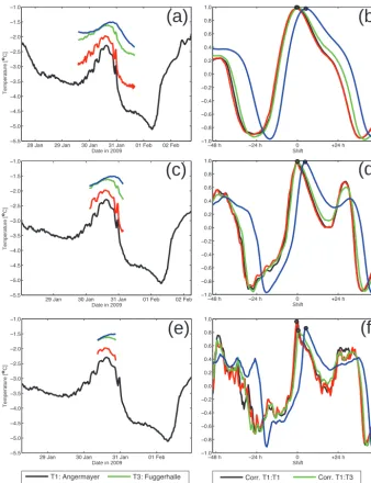
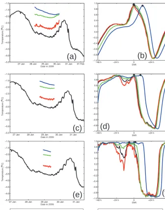
To find an adequatenit is helpful to actually take a look at the correlation function of example data observed in Schel-lenberger Eishöhle. We analyzed temperatures observed by four different loggers during periods of large temperature variations on 30 January (Fig. 4) or small temperature varia-tions on 29 January (Fig. 5). The temperatures at logger T1 were taken as a reference, while the temperatures recorded by loggers T2, T3, and T4 were cross-correlated with the temperatures at logger T1 using different numbers of sam-ples. During periods with large temperature variations, only a small number of samples is needed to produce distinc-tive maxima in the correlation function (Fig. 4, bottom pan-els). Actually for our example epoch, correlation maxima are more distinctive the fewer samples are used. During periods of little temperature variations on the other hand, no distinc-tion of a maximum of correladistinc-tion is possible, if too few sam-ples n are considered for cross-correlation (Fig. 5, middle and bottom panels) and the determined time shifts become meaningless. Generally we may assume that a time span of 1 day (corresponding roughly to a correlation lengthnof 51 samples in Figs. 4 and 5) will most probably suffice in most cases to get a clear correlation peak due to the day/night cy-cle in outside temperature. Shorter time spans may suffice during periods of pronounced weather patterns. Fine tuning ofnwill be worthwhile, whenever time resolution of the de-termined airflow speeds is in the center of interest.

The second parameter we have to choose is the maximum number of samples we shift time seriesY against time series

(6)

win-29 Jan 30 Jan 31 Jan 01 Feb

−5.5 −5.0 −4.5 −4.0 −3.5 −3.0 −2.5 −2.0 −1.5 −1.0

Date in 2009

29 Jan 30 Jan 31 Jan 01 Feb 02 Feb

−5.5 −5.0 −4.5 −4.0 −3.5 −3.0 −2.5 −2.0 −1.5 −1.0

Date in 2009

28 Jan 29 Jan 30 Jan 31 Jan 01 Feb 02 Feb

−5.5 −5.0 −4.5 −4.0 −3.5 −3.0 −2.5 −2.0 −1.5 −1.0

Date in 2009

Temperature

[

C]

−48 h −24 h 0 +24 h +48 h

−1.0 −0.8 −0.6 −0.4 −0.2 0.0 0.2 0.4 0.6 0.8 1.0

Shift

−48 h −24 h 0 +24 h +48 h

−1.0 −0.8 −0.6 −0.4 −0.2 0.0 0.2 0.4 0.6 0.8 1.0

Shift

−48 h −24 h 0 +24 h +48 h

−1.0 −0.8 −0.6 −0.4 −0.2 0.0 0.2 0.4 0.6 0.8 1.0

Shift

Corr. T1:T1

Corr. T1:T2 Corr. T1:T3Corr. T1:T4 T1: Angermayer

T2: Wasserstelle T3: FuggerhalleT4: Angermayer

(a)

(b)

(c)

(d)

(e)

(f)

Temperature

[

C]

Temperature

[

C]

Figure 4. Observed temperatures (left panels) and correlation functions (right panels) during a period of large temperature variations, well suited for correlation analysis. Data of loggers T2, T3, or T4 are cross-correlated with the data of logger T1 using a correlation length of 101 (a, b), 51 (c, d), and 25 (e, f) samples.

dows of ±2 d to also show the variability of the correlation coefficient related to the applied time shift.

It has to be stressed that the sampling rate of the temper-ature measurements limits the time resolution of the corre-lation analysis. The time shift of maximum correcorre-lation will always be an integer multiple of the sampling rate, and its uncertainty corresponds to half the sampling rate. Even if the smooth nature of the temperature measurements suggests creasing the sampling rate by interpolation, this will not in-troduce new information for the correlation analysis. On the other hand, it does not disturb the analysis according to our experience (not shown).

4.2 Bias and scale

The time shifts determined by the correlation analysis are inserted into Eq. (4) to compute the partial derivatives with respect to the scale factors. In a consecutive step, biases and scale factors of our simple model can be determined for each pair of data loggers. We perform the least-squares adjustment for the example epoch of Fig. 4, applying the time shifts de-termined using 51 samples (Fig. 4, middle row).

(7)

exam-−48 h −24 h 0 +24 h +48 h −1.0

−0.8 −0.6 −0.4 −0.2 0.0 0.2 0.4 0.6 0.8 1.0

Shift

−48 h −24 h 0 +24 h +48 h −1.0

−0.8 −0.6 −0.4 −0.2 0.0 0.2 0.4 0.6 0.8 1.0

Shift

−48 h −24 h 0 +24 h +48 h −1.0

−0.8 −0.6 −0.4 −0.2 0.0 0.2 0.4 0.6 0.8 1.0

Shift

27 Jan 28 Jan 29 Jan 30 Jan 31 Jan −5.5

−5.0 −4.5 −4.0 −3.5 −3.0 −2.5 −2.0 −1.5 −1.0

Date in 2009

27 Jan 28 Jan 29 Jan 30 Jan 31 Jan −5.5

−5.0 −4.5 −4.0 −3.5 −3.0 −2.5 −2.0 −1.5 −1.0

Date in 2009

27 Jan 28 Jan 29 Jan 30 Jan 31 Jan 01 Feb −5.5

−5.0 −4.5 −4.0 −3.5 −3.0 −2.5 −2.0 −1.5 −1.0

Date in 2009

Corr. T1:T1

Corr. T1:T2 Corr. T1:T3Corr. T1:T4

T1: Angermayer

T2: Wasserstelle T3: FuggerhalleT4: Angermayer

(a)

(b)

(c)

(d)

(e)

(f)

Temperature

[

C]

Temperature

[

C]

Temperature

[

C]

Figure 5. Observed temperatures (left panels) and correlation functions (right panels) during a period of small temperature variations, apparently not so well suited for correlation analysis. Data of loggers T2, T3, or T4 are cross-correlated with the data of logger T1 using a correlation length of 101 (a, b), 51 (c, d), and 25 (e, f) samples.

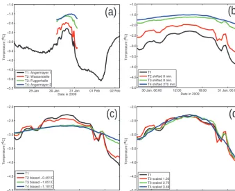
ple epoch are listed in the legends of Figs. 6 and 7. To com-pare them, the signs of the time shift and bias of either Figs. 6 or 7 have to be changed and the corresponding scale has to be inverted. Note that bias and scale factor were determined together and are only evaluated separately for Figs. 6 and 7.

Between loggers T1 and T2 the air is warmed by 0.45◦C (or 0.47◦C); between T1 to T3 it is warmed by 1.05◦C, and between T1 and T4 by 1.12◦C (or 1.19◦C). This warming goes hand in hand with an attenuation of temperature varia-tions by a factor of 0.77 (or 1/1.22) between T1 and T2, by a factor of 0.36 (or 1/2.75) between T1 and T3, and by a factor of 0.31 (or 1/3.49) between T1 and T4. We therefore assume that the inflowing cold air passes T1 and T2 on its way to the

(8)

29 Jan 30 Jan 31 Jan 01 Feb 02 Feb

−5.5 −5.0 −4.5 −4.0 −3.5 −3.0 −2.5 −2.0 −1.5 −1.0

Date in 2009

T1: Angermayer 1 T2: Wasserstelle T3: Fuggerhalle

T4: Angermayer 2

30 Jan, 06:00 12:00 18:00 31 Jan, 00:00

−5.0 −4.5 −4.0 −3.5 −3.0 −2.5 −2.0 −1.5 −1.0

Date in 2009

T1

T2 shifted 0 min. T3 shifted 0 min. T4 shifted 270 min.

30 Jan, 06:00 12:00 18:00 31 Jan, 00:00

−5.0 −4.5 −4.0 −3.5 −3.0 −2.5 −2.0

Date in 2009

T1

T2 biased −0.45ϒ C

30 Jan, 06:00 12:00 18:00 31 Jan, 00:00

−5.0 −4.5 −4.0 −3.5 −3.0 −2.5 −2.0

Date in 2009

T1

T2 scaled 1.22 T3 scaled 2.75 T4 scaled 3.49

(a)

(b)

(c)

(d)

Temperature

[

C]

Temperature

[

C]

Temperature

[

C]

Temperature

[

C]

Figure 6. Raw data (a) of loggers T2, T3, and T4 were shifted in time relative to logger T1 to be correlated (b). The time period shown in (a) corresponds to the search window, while a time span of 51 samples was used for correlation analysis and to adjust temperature biases and scale factors. In a second step (c) the temperature biases were applied to loggers T2, T3, and T4; and finally (d) the temperature variations at loggers T2, T3, and T4 were scaled to fit those at logger T1.

its way through the cave and the attenuation of temperature variations agree well with the assumptions that underlie the model design (see Sect. 3).

The slightly different results in Figs. 6 and 7 are due to the fact that the reference epochs differ by the determined time shifts (depending on which logger is kept fixed as reference). The very much comparable results prove that the method is robust and that the parameters are stable for the period un-der investigation (the temporal variability of the parameters is studied in Sect. 5). The validity of our model is further confirmed by the optically good fit achieved for the example data (Figs. 6d and 7d); measures for the quality of the model fit are introduced in Sect. 6.

5 Temporal variability

In Sect. 4.1 it was mentioned that the airflow speed is sup-posed to be constant during the time period considered for correlation. In this section we will estimate airflow speeds (time shifts) for the whole period of about 6 days (see Fig. 3) to check if this requirement is met. To do so we repeat the analysis performed in Sect. 4 for an example epoch for all epochs of the period shown in Fig. 3. We use either 51 or 101 samples for correlation. We also try the effect of

smooth-ing (by a centered movsmooth-ing mean of five samples) to filter out short-term variations of unknown origin visible in Fig. 3.

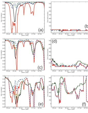
The determined time shifts and the corresponding max-ima of correlation are displayed in Fig. 8. The latter may serve to assess the reliability of the time shifts. Compara-bly small correlation coefficients indicate questionable re-sults. Only between loggers T1 and T2 the correlation, at least of the smoothed temperature data, is high during the whole period analyzed and the determined airflow speed is quite constant. As already mentioned, the sampling rate of 30 min is too coarse to really resolve it; the time shift varies between 0 and−30 min, indicating a true value between both limits. The negative time shift, which is at first glance puz-zling, may hint at the placement of logger T1 too high above the ground. The cold air entering the cave moves along the floor of the passage below T1 and reaches T2, before it is recorded by T1 (see discussion in Sect. 7).

(9)

correla-29 Jan 30 Jan 31 Jan 01 Feb 02 Feb

−5.0 −4.5 −4.0 −3.5 −3.0 −2.5 −2.0 −1.5 −1.0

Date in 2009

T1: Angermayer 1 T2: Wasserstelle T3: Fuggerhalle

T4: Angermayer 2

30 Jan, 06:00 12:00 18:00 31 Jan, 00:00

−5.0 −4.5 −4.0 −3.5 −3.0 −2.5 −2.0 −1.5 −1.0

Date in 2009

T2

T1 shifted 30 min.

T3

T1 shifted 0 min. T4

T1 shifted −270 min.

30 Jan, 06:00 12:00 18:00 31 Jan, 00:00

−4.0 −3.5 −3.0 −2.5 −2.0 −1.5 −1.0

Date in 2009

T2

T1 biased 0.47ϒ C T3

T1 biased 1.05ϒ C

T4 T1 biased 1.12ϒ C

30 Jan, 06:00 12:00 18:00 31 Jan, 00:00

−4.0 −3.5 −3.0 −2.5 −2.0 −1.5 −1.0

Date in 2009

T2

T1 scaled 0.77

T3

T1 scaled 0.36 T4 T1 scaled 0.31

(a)

(b)

(c)

(d)

Temperature

[

C]

Temperature

[

C]

Temperature

[

C]

Temperature

[

C]

Figure 7. In this example the raw data (a) of logger T1 were shifted (b) relative to loggers T2, T3, or T4 until best correlation was reached. Then (c) temperature biases were applied at logger T1 to fit either T2, T3, or T4 before finally, (d) the temperature variations at logger T1 were scaled to fit loggers T2, T3, or T4.

tion analysis fails. The somewhat different values determined from the analysis of either 51 or 101 samples indicate that the slow airflow at the beginning of the period affects the results for a longer time if 101 samples are considered for correla-tion. In general the correlation of a larger number of samples leads to smoother results. In case of the analysis of loggers T1 and T4 we get very variable results for the time shifts as well as for the value of maximum correlation. A closer look at the correlation function at single epochs would reveal that side maxima distort the analysis, leading to jumps in the determined time shifts. A reduction of the search window would probably help to remove some of these artifacts. The results achieved for 51 or 101 samples agree best during the middle of the period, where the spell of warm weather leads to a distinct temperature pattern that facilitates the correla-tion analysis. The smoothing of the data generally improves correlation by reduction of uncorrelated noise, but does not significantly alter the determined time shifts.

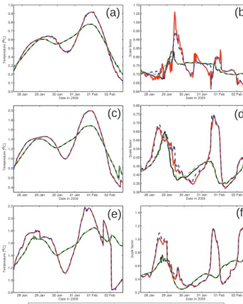
After applying the determined time shifts to the time series of temperature observations at loggers T2, T3, and T4, opti-mal biases and scale factors were estimated for each epoch. The results are summarized in Fig. 9 and show a strong de-pendency on the temperature of the cold inflowing air. Colder inflowing air goes hand in hand with larger temperature gra-dients that lead to a faster inflow of the cold air. This

re-sults in less pronounced attenuation of temperature varia-tions, i.e., larger scale factors, because the time for energy exchange with the cave (air, ice, rock) is reduced. The short spell of warm weather on 30 January immediately leads to an increased attenuation, i.e., smaller scale factors. The bi-ases increase with the steepness of the temperature gradients. Again, the parameters were fitted either from 51 temperature samples or from 101 samples. Because the fit is optimal to all samples used, an averaging takes place and the results obtained from more samples look considerably smoother. A smoothing (moving mean) of the temperature time series prior to the estimation of biases and scales helped to derive scales between T1 and T2, where short-term variations of unknown origin superimpose the temperature variability in-duced by outside temperature variation (Fig. 9b).

6 Validation of the model

(10)

28 Jan 29 Jan 30 Jan 31 Jan 01 Feb 02 Feb 0.90

0.91 0.92 0.93 0.94 0.95 0.96 0.97 0.98 0.99 1.00

Date in 2009

Max. correlation

28 Jan 29 Jan 30 Jan 31 Jan 01 Feb 02 Feb 0

100 200 300 400 500 600 700

Date in 2009

Time shift [minutes]

0.91 0.92 0.93 0.94 0.95 0.96 0.97 0.98 0.99 1.00

Date in 2009

Max. correlation

100 200 300 400 500 600 700

Date in 2009

0.91 0.92 0.93 0.94 0.95 0.96 0.97 0.98 0.99 1.00

Date in 2009

Max. correlation

100 200 300 400 500 600 700

Date in 2009

n=101 n=51 n=101, smoothed n=51, smoothed

(a)

(b)

(c)

(d)

(e)

(f)

Figure 8. Epoch-wise maxima of correlation (left panels) and corresponding time shifts (right panels) for the three pairs of loggers T1 : T2 (top panels), T1 : T3 (middle panels), and T1 : T4 (bottom panels); for smoothing the centered moving mean of five samples was computed.

assumed. In our analysis of data collected in Schellenberger Eishöhle, correlation was generally high (>0.9 for most of the time analyzed) and we can safely assume the linear model to be valid. The quality of the bias and scale parameters de-termined by a least-squares adjustment can be assessed by their formal errors. The overall quality of the model is char-acterized by the post-fit error of the modeled temperatures when compared to the ones actually observed.

The post-fit errorσ of the modeled temperatures is easily computed from the sum of squares of the residuals:

ν2=X

n

(TB, observed−TB, modeled)2 (8)

σ=

s ν2

n−u, (9)

(11)

0.1 0.2 0.3 0.4 0.5 0.6 0.7 0.8 0.9 1.0

Date in 2009 28 Jan 29 Jan 30 Jan 31 Jan 01 Feb 02 Feb

0.60 0.65 0.70 0.75 0.80 0.85 0.90 0.95 1.00 1.05 1.10

Date in 2009

Scale factor

0.6 0.8 1.0 1.2 1.4 1.6 1.8 2.0

0.30 0.35 0.40 0.45 0.50 0.55 0.60 0.65 0.70 0.75 0.80

Date in 2009

Scale factor

1.0 1.2 1.4 1.6 1.8 2.0 2.2

0.2 0.4 0.6 0.8 1.0 1.2 1.4

Date in 2009

Scale factor

(a)

(b)

(c)

(d)

(e)

(f)

Temperature

[

C]

Temperature

[

C]

Temperature

[

C]

Figure 9. Epoch-wise biases (left panels) and scale factors (right panels) for the three pairs of loggers T1 : T2 (top panels), T1 : T3 (middle panels), and T1 : T4 (bottom panels); for smoothing the centered moving mean of five samples was computed.

The formal errors of biasσband scale factorσsare taken from the covariance matrix of the least-squares adjustment:

K=σ2·

σ_b2 σbs

σsb σs2

=σ2·ATPA

−1

. (10)

K is a symmetric matrix; covariancesσbsandσsbare identi-cal. Keep in mind that in Sect. 3 we chose P to be the identity matrix. The formal errors are scaled by the post-fit errorσ. Note that from the covariance matrix one can also compute the correlation coefficient between the bias and the scale fac-tor:

rbs=

σbs √

σb·σs

. (11)

This has not been evaluated in this study. In the case of the data analyzed from Schellenberger Eishöhle the correlation between bias and scale turned out to be small and could also be neglected (corresponding to a separate estimation of both parameters).

(12)

0.005 0.010 0.015 0.020 0.025 0.030

Date in 2009

S

ig

m

a:

te

m

pe

ra

tu

re

b

ia

s [

C

]

0.000 0.005 0.010 0.015 0.020 0.025 0.030

Date in 2009

0.000 0.005 0.010 0.015 0.020 0.025 0.030

Date in 2009

0.00 0.05 0.10 0.15 0.20 0.25

Date in 2009

Sigma: scale factor

0.00 0.05 0.10 0.15 0.20 0.25

Date in 2009

Sigma: scale factor

0.00 0.05 0.10 0.15 0.20 0.25

Date in 2009

Sigma: scale factor

(a)

(b)

(c)

(d)

(e)

(f)

Sigma:

temperature

bias

[

C]

Sigma:

temperature

bias

[

C]

Figure 10. Epoch-wise standard deviations of biases (left panels) and scale factors (right panels) for the three pairs of loggers T1 : T2 (top panels), T1 : T3 (middle panels), and T1 : T4 (bottom panels).

As long as the time shifts are computed independently by cross-correlation we cannot define their error bounds corre-spondingly to bias and scale. However, in any case the ac-curacy of the determined time shifts is limited by the pling rate of the temperature observations to half the sam-pling interval (in our case, this corresponds to error bounds of plus/minus 15 min). Note that time shifts determined to be zero are not meaningless; they just show that the air took less time than half the sampling period (i.e., 15 min) from one logger to another.

Finally the significance of the estimated parameters may be calculated, assuming that their errors are normally dis-tributed (their variances areχ2-distributed). This test tells us

if the parameter in question is indispensable to improve the model. We expect that during the closed phase, only the bi-ases are significant parameters of the model (corresponding to time shifts of 0 and scales of 1 that do not contribute to the modeled temperatures), while during the open phase all three parameters are rated as significant. The test of signif-icance will not tell us if the estimated values represent the physical quantities the parameters were intended to model. A parameter that absorbs systematic noise will be rated as significant, even if the determined numerical values may not be interpreted in a meaningful way.

(13)

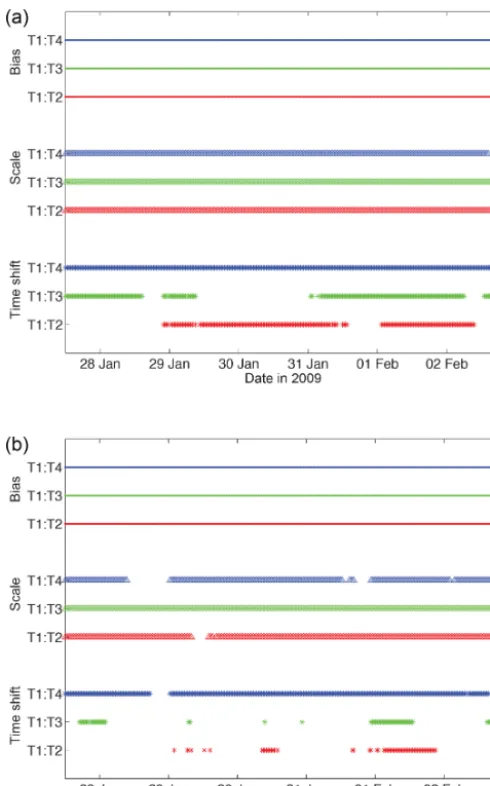
Figure 11. Significantly determined parameters; correlation length is 101 samples (a) or 51 samples (b).

(full model), the other one including all but the parameter in question (reduced model).

The reduced model to test the significance of1treads

TB1t(t )=s·(TA(t )−TA)+b

∗_; ₍₁₂₎

the reduced model to test the significance ofsreads

TBs(t )=TA(t−1t )+b

∗_;

(13) and finally, the reduced model to test the significance ofb∗

reads

TBb∗(t )=s·(TA(t−1t )−TA)+TA. (14)

Note that it is not correct to determine the parameters of the full model once and subsequently insert them into the re-duced models. Instead, the parameters of each of the rere-duced models have to be determined in a separate estimation pro-cedure to also take into account the correlations between the

different parameters. As mentioned before, the correlations may be neglected here for the test of bias and scale, which can be determined quite independently, but for the signifi-cance test of the time shift, both parameters of the reduced model (Eq. 12) have to be re-estimated with a time shift of

1t=0.

We perform anF test (e.g., Snedecor and Cochrane, 1989) computing the ratio

8= ν

2 r −νf2

/(rr−rf)

ν_f2/rf

, (15)

whereν_r2andν_f2are the sum of squares of the observed tem-peratures after substraction of the modeled ones (see Eq. 8); subscript f refers to the full model, subscript r to the reduced model.rr andrf are the corresponding degrees of freedom

n−uof the two models, the number of unknownsur=uf−1 of the reduced model being smaller than that of the full model

uf, and thereforerr=rf+1.

8 is F-distributed, its probability density function

Fnm(8), with n=rf andm=rr−rf, is a measure for the probability that the additional parameter in the full model could have been estimated in the same way from normally distributed random numbers. We evaluate the associated cu-mulative distribution function and reject all parameters for which it is smaller than 0.99 (corresponding to a 99 % con-fidence level). The remaining biases, scales, and time shifts are marked in Fig. 11a for a correlation length of 101 sam-ples, and in Fig. 11b for a correlation length of 51 samples. Bias and scale turn out to significantly improve the model for most of the time. The results look different for the time shift, which is only rated as significant for short periods of time. Comparing Fig. 11 with Fig. 8 we realize that the time shift is always rated insignificant when it is estimated to be zero. This is reasonable because a time shift of zero corresponds to not estimating the time shift at all. As stated above, the estimates of zero for the time shift are artifacts caused by the coarse sampling rate. With an increased sampling rate, it can be expected that the time shifts are rated as significant whenever the scale factors that benefit from the high temper-ature resolution of the loggers indicate air movements in the cave. The message of Fig. 11 therefore is that for the time period analyzed, all three parameters – time shift (as soon as it is larger than half the sampling rate), bias, and scale – are indispensable for our model. The test probably will become more interesting when the model is refined to include effects like insolation of the entrance hall that most probably affects the loggers in Angermayerhalle and should be measurable, at least during the closed phase of the cave.

7 Discussion of results

(14)

described in Meyer et al. (2014), the two loggers T1 and T4 in Angermayerhalle show very different behavior (Fig. 7a) that could not yet be explained. Our analysis revealed a sig-nificant time shift (Fig. 7b) as well as a pronounced posi-tive temperature bias (Fig. 7c) of T4 relaposi-tive to T1, as well as a pronounced attenuation of the temperature variations (Fig. 7d) recorded by T4. We therefore assume that logger T1 records the cold inflowing air, while T4 records the rela-tively warmer air flowing out of the cave. We further assume that the cold inflowing air passes by logger T2 to the deepest point in Fuggerhalle, where logger T3 is positioned. Temper-ature biases are positive and increase with the distance the air has traveled into the cave (as long as we assume that T4 records the outflowing air), as predicted by our model. The scaling factors are smaller than 1 (attenuation of signal) and are inversely proportional to the distance the air has traveled. The sampling rate of 30 min proved to be too coarse to determine the airflow speed from T1 to T3 for most of the time analyzed. The estimate of 0 min means that the air took less than 15 min for the distance of approximately 65 m be-tween T1 and T3, corresponding to a speed of more than 4 m min−1 (agreeing well with air speeds of gravitational flow of 6 m min−1 reported by Smithson, 1991). Negative values for the time shift between T1 and T2 may indicate a position of logger T1 too high above the floor so that the cold air that flows along the floor of the passage passes T1 without being noticed and reaches T2 before it is recorded at T1. This suspicion was confirmed by in situ inspection of logger T1.

While T2 shows distinctive variations of rather short du-ration (and unknown origin) that clearly correspond to the temperature variations recorded by T1, the same variations are very much attenuated at T3 and not at all visible any more at T4. This may be explained by the distance the air traveled inside the cave and by the attenuation of the temper-ature variations due to energy exchange with stagnant cave air, ice, and rock. Moreover, Fuggerhalle acts as a dead end where the cold air that enters via Wasserstelle and probably also via Mörkdom is thoroughly mixed with the stagnant air. The assumption that Fuggerhalle is probably warmed by dy-namic ventilation from deeper reaches of the cave could not be confirmed. The temperature biases and scaling factors de-termined for T3 fit our model very well. We conclude that Fuggerhalle is warmer than Angermayerhalle or Wasserstelle just because it is farther from the entrance.

From T3 at the furthest end of Fuggerhalle the warm air takes a significant amount of time before it reaches T4 on its way out of the cave. For this remaining distance of 115 m, a time shift of 270 min was determined for our example epoch (Sect. 4.1), corresponding to an air speed of 0.5 m min−1. Not much more signal attenuation or warming takes place along this path. Unfortunately, in the time period analyzed, no log-ger was positioned in the second passage (Mörkdom) con-necting Angermayerhalle and Fuggerhalle, so it cannot be clarified if one of the passages acts as the primary way down

for the cold air while the other channels the warm air back to the surface. The determined air speeds have to be considered as mean speeds for the way the air traveled between loggers; they will of course vary depending on the cross section of the passage. The different speeds determined for the inflow-ing cold air and the replaced warm air may also be explained by the cross section of the passage occupied by the corre-sponding air flow. Independent of all the factors that compli-cate interpretation, we can state that the results appear to be realistic.

The resolution of the correlation analysis is drastically lim-ited by the coarse sampling rate of the loggers and the miss-ing synchronization. This fact does not reduce the applica-bility or validity of our model, but it limits the interpreta-tion of the results. Nevertheless we were able to characterize the general patterns of air movement and their slow tempo-ral variations. The analysis of the tempotempo-ral variability of the determined parameters (Sect. 5) confirmed the basic princi-ples on which the model is based. Low outside temperatures correspond to steep temperature gradients that result in small time shifts (high air speeds). The energy exchange with the cave environment is limited by the short time the cold air stays in the cave, and the attenuation factors are closer to 1 when outside temperatures are low. The biases correspond to the temperature gradients and are larger during spells of cold weather.

But the analysis of the temporal variability also revealed problems in the correlation analysis. The cross-correlation of loggers T1 and T4 exhibits an unrealistic variability, in-cluding a number of jumps. These clearly are artifacts that are caused by side maxima of the correlation analysis, stress-ing the need to limit the search window to a sensible width, which depends on the cave, the placement of the loggers, and the distance between loggers, and can only be refined after some tentative analysis. Generally it can be stated that times of poor correlation correspond to periods of little temperature variations. Long correlation lengths may help but also reduce the time resolution of the determined time shifts due to av-eraging over the number of samples used for the correlation analysis. A rise of the outside temperatures above the cave temperature will lead to ceasing air flow and an interruption in the open phase of the cave. In this case the correlation analysis fails.

(15)

out-side winds would be a probable candidate, though difficult to model. As is the case for the time shifts, a reduced number of samples used for the determination of bias and scale fac-tor leads to an improved time resolution, while an increased number of samples stabilizes the estimation. As can be ex-pected, the uncertainty of the fit (i.e., the formal errors of bias and scale factor) increases with the distance between loggers.

8 Conclusions

The objective of this paper is to present the principles and the methodology of the calcFLOW method that was devel-oped in order to be able to use air temperature measurements in static ice caves to define the airflow regime. The idea of calcFLOW is based on the fact that in many ice caves in re-mote places, airflow measurements are difficult. However, in every ice cave where cave climate related studies are con-ducted, at least temperature measurements (air, rock, ice) are performed. Based on this data we calculate three different parameters to better characterize the processes that dominate the cave climate and to understand the temperature differ-ences observed between the measuring points: the airflow speed, the change of the mean air temperature, and the at-tenuation of the temperature variations dependent on the lo-cation inside the cave. The primary objective is to calculate airflow speeds inside a static ice cave to define the airflow regime. It is achieved by cross-correlating air temperature data of different logger sites. The method was applied to temperatures recorded in Schellenberger Eishöhle during the open period, when air movement inside the cave is governed by gravitational flow.

The method of cross-correlation we use for the determi-nation of time shifts in general depends on rather distinc-tive temperature variations to successfully correlate the ob-servations of different loggers. On the other hand, the airflow speed is supposed to be relatively constant during the time span used for correlation. These two requirements contradict each other and it has to be shown by further studies to what extent the temporal variability of the air movements inside the cave may be resolved. Most probably the reliability of the analysis will benefit from an increased sampling rate of the temperature observations. Regardless of the complexity of the situation at our test site, we may state that the pre-sented method is well suited to uncover the complicated air movements in the cave. The results of the analysis will help to optimize the placement of the loggers. An increased num-ber of loggers positioned near the floor as well as near the ceiling of the passages will allow the paths of the inflowing and outflowing air to be distinguished with much better spa-tial resolution and reliability. Decreased sampling intervals will enable the determination of the speed of the rather fast inflowing cold air and generally improve the reliability of the correlation analysis.

We have already tested calcFLOW with air temperature data from Fossil Mountain Ice Cave (USA), but these results will be part of future publications. What we can already state for the moment is that calcFLOW is applicable to other ice caves, too. This is one major reason for the publication of this pilot study and also a reason for us to keep the model as simple as possible. We want to present a basic tool for cave climate studies which everyone can use for their specific site. To summarize the outcome of this study, we can state that calcFLOW is useful in the following way:

1. to characterize the airflow regime inside a static ice cave;

2. to compute (interpolate) the temperatures between two loggers with one simple model, based on only three de-termined parameters;

3. to indicate possible problems in the measuring setup (e.g., position and height of loggers); and

4. to indicate useful observation intervals.

In a next step we will address key problems of calcFLOW in a dedicated simulation study with the objective to provide measures for the signal content of the time series of tempera-ture observations, evaluated by the root-mean-square, and for the quality of the cross-correlation. The latter will be based on the shape of the peak of maximum correlation, exploit-ing characteristics like its dominance and width. The simu-lation study will also provide a test bed for cross-validation methods to assess the reliability of the determined air speeds; and of course we also hope to validate the calculated airflow speeds by comparison to real-time airflow measurements.

Meanwhile the logger setup in Schellenberger Eishöhle has been revised. With the expected results we hope to be able to further differentiate the specific paths of the airflow and to tackle questions of energy exchange in the cave. For this task, finally a much denser network of temperature log-gers, which also probe ice and rock temperatures, and a vol-ume model of the cave and its ice filling, will be indispens-able. The evaluation of the temperature observations has to be automatized, based on the criteria developed in the simu-lation study.

Acknowledgements. This work is part of the Italian Project of

Strategic Interest NEXTDATA (PNR2011–2013) funded by the Italian National Research Council (CNR). It is also part of a PhD project, “Ice deposit evolution and cave climatology of ice caves”, at Ruhr University Bochum (Germany). For the logistical support and the good cooperation, we would like to thank the Verein für Höhlenkunde Schellenberg e.V. Moreover, we would like to thank Martina Grudzielanek for the revision of the mathematical part of the paper.

(16)

References

Bock, H.: Mathematisch-physikalische Untersuchung der

Eishöhlen und Windröhren, in: Die Höhlen im Dachstein, Verein für Höhlenkunde in Österreich, Graz, 102–144, 1913. Bögli, A.: Karsthydrographie und physische Speläologie, Berlin,

1978.

Crammer, H.: Eishöhlen- und Windröhren-Studien, in: Abhand-lungen der K. K. geographischen Gesellschaft in Wien, Vol. 1, K. K. geographical society of Vienna, printed by Verlag Lechner, Wien, 1899.

Fugger, E.: Beobachtungen in den Eishöhlen des Untersberges bei Salzburg, Mitteilungen der Gesellschaft für Salzburger Lan-deskunde (MGSLK), Salzburg, 28, 65–144, 1888.

Grebe, C.: Eishöhlenforschung vom 16. Jahrhundert bis in die Mod-erne – vom Phänomen zur aktuellen Forschung, MS thesis, un-published, Bochum, Germany, 2010.

Grebe, C., Ringeis, J., and Pflitsch, A.: Study of Temperature and Airflow in the Schellenberger Ice Cave (Berchtesgadener Limestone Alps, Germany), in: Proceedings of 3rd International Workshop on Ice Caves (IWIC-III), Kungur Ice Cave, Perm Re-gion, Russia, 12–17 May 2008, 26–29, 2008.

Koch, K. R.: Parameter Estimation and Hypothesis Testing in Lin-ear Models, 2nd Edn., Springer, Berlin, Heidelberg, New York, 1999.

Korzystka, M., Piasecki, J., Sawinski, T., and Zelinka, J.: Cli-matic system of the Dobinska Ice Cave, in: Proceedings of the 6th Congress International Show Caves Associations, Liptovsky Mikulas, 85–97, 2011.

Laroque, M., Mangin, A., Razack, M., and Banton, O.: Contribution of correlation and spectral analyses to the regional study of a large karst aquifer (Charente, France), J. Hydrol., 205, 217–231, 1998.

Lohmann, H.: Das Höhleneis unter besonderer Berücksichtigung einiger Eishöhlen des Erzgebirges, Diss., Univ. Leipzig, Leipzig, 1895.

Lütscher, M. and Jeannin, P. Y.: Une anne d’enregistrements de tem-peratures la glaciere de Monlesi/Ein Jahr Temperaturmessungen in der Glaciere de Monlesi (NE), Stalactite, 52, 27–29, 2002. Lütscher, M. and Jeannin, P. Y.: A process-based classification of

alpine ice caves, Theor. Appl. Karstol., 17, 5–10, 2004a. Lütscher, M. and Jeannin, P. Y.: The role of winter air circulation for

the presence of subsurface ice accumulations: an example from Monlesi Ice Cave (Switzerland), Theor. Appl. Karstol., 17, 19– 25, 2004b.

Lütscher, M.: Processes in Ice Caves and their Significance for Pa-leoenvironmental Reconstructions, Thesis university of Zürich, edition ISSKA, La Chaux-de-Fonds, 2005.

Meyer, C., Pflitsch, A., Holmgren, D., and Maggi, V.: Schellen-berger Ice Cave (Germany): a conceptual model of temperature and airflow, in: Proceedings of the Sixth International Workshop on Ice Caves, 17–22 August, Idaho Falls, Idaho, USA, 82–87, 2014.

Morard, S., Bochud, M., and Delaloye, R.: Rapid changes of the ice mass configuration in the dynamic Diablotins ice cave – Fribourg Prealps, Switzerland, The Cryosphere, 4, 489–500, doi:10.5194/tc-4-489-2010, 2010.

Padilla, A. and Pulido-Bosch, A.: Study of hydrographs of karstic aquifers by means of correlation and cross-spectral analysis, J. Hydrol., 168, 73–89, 1994.

Pflitsch, A. and Piasecki, J.: Detection of an airflow system in Niedzwiedzia (Bear) Cave, Kletno, Poland, J. Cave Karst Stud., 65, 160–173, 2003.

Pflitsch, A., Piasecki, J., and Sawinski, T.: Development and degra-dation of ice crystals sediment in Dobsinska Ice Cave (Slovakia), in: 2nd International Workshop on Ice Caves IWIC II, Proceed-ings, 8–12 May, Demänovska Dolina, Slovak Republic, Lip-tovsky Mikulas, 29–37, 2007.

Racovitza, G.: Observations sur la glacière naturelle dite Ghetarul de la Scarisoara’, Bull. Soc. Sci. Cluj., III, 75–108, 1927. Racovitza, G.: La classification topoclimatique des cavités

souter-raines, in: Trav. Inst. Speol. “E. Racovitza”, 14, 197–216, 1975. Racovitza, G. and Onac, B. P.: Scarisoara Glacier Cave, Monografic

study, Ed. Carpatica, Cluj-Napoca, 2000.

Saar, R.: Eishöhlen, ein meteorologisch-geophysikalisches

Phänomen, Untersuchungen an der Rieseneishöhle (R.E.H.) im Dachstein, Oberösterreich, in: Geogr. Ann. A, 38, 1–63, 1956. Smithson, P. A.: Inter-relationship between cave and outside air

temperatures, Theor. Appl. Climatol., 44, 65–73, 1991. Snedecor, G. W. and Cochrane, W. G.: Statistical Methods, 8th Edn.,

Iowa State University Press, Ames, 1989.