www.earth-surf-dynam.net/4/607/2016/ doi:10.5194/esurf-4-607-2016
© Author(s) 2016. CC Attribution 3.0 License.
Exploring the sensitivity on a soil area-slope-grading
relationship to changes in process parameters using a
pedogenesis model
W. D. Dimuth P. Welivitiya1,2, Garry R. Willgoose1, Greg R. Hancock2, and Sagy Cohen3 1School of Engineering, The University of Newcastle, Callaghan, 2308, Australia
2School of Environment and Life Sciences, The University of Newcastle, Callaghan, 2308, Australia 3Department of Geography, University of Alabama, P.O. Box 870322, Tuscaloosa, Alabama 35487, USA
Correspondence to:Garry R. Willgoose ([email protected])
Received: 24 December 2015 – Published in Earth Surf. Dynam. Discuss.: 20 January 2016 Revised: 25 April 2016 – Accepted: 13 May 2016 – Published: 1 August 2016
Abstract. This paper generalises the physical dependence of the relationship between contributing area, lo-cal slope, and the surface soil grading using a pedogenesis model and allows an exploration of soilscape self-organisation. A parametric study was carried out using different parent materials, erosion, and weathering mech-anisms. These simulations confirmed the generality of the area-slope-d50 relationship. The relationship is also true for other statistics of soil grading (e.g.d10,d90) and robust for different depths within the profile. For small area-slope regimes (i.e. hillslopes with small areas and/or slopes) only the smallest particles can be mobilised by erosion and the area-slope-d50relationship appears to reflect the erosion model and its Shield’s Stress threshold. For higher area-slope regimes, total mobilization of the entire soil grading occurs and self-organisation reflects the relative entrainment of different size fractions. Occasionally the interaction between the in-profile weather-ing and surface erosion draws the bedrock to the surface and forms a bedrock outcrop. The study also shows the influence on different depth-dependent in-profile weathering functions in the formation of the equilibrium soil profile and the grading characteristics of the soil within the profile. We outline the potential of this new model and its ability to numerically explore soil and landscape properties.
1 Introduction
Soil is a product of various physical processes acting on earth’s crust. Weathering is a major contributor to soil pro-duction, along with transport processes that transport new material away and bring new material into a point. Weather-ing is a general term used to describe all the processes which cause rocks or rock fragments to disintegrate or alter through physical (Ollier, 1984; Wells et al., 2006, 2008; Yokoyama and Matsukura, 2006), chemical (Green et al., 2006; Ollier, 1984) or biological means (Strahler and Strahler, 2006). Dis-integration of rock material through physical weathering can occur by (1) unloading, (2) expansion and contraction of rock through heating and cooling cycles, (3) stress developing in rock fractures due to freezing water, (4) salt crystal growth or tree root intrusions, and (5) abrasion of rock by harder
materials transported by flowing water or glaciers (Thorn-bury, 1969). Physical weathering where larger soil particles are broken down into smaller particles is dominant in the surface layer of material where it is more exposed. Weath-ering also occurs underneath the surface and the weathWeath-ering rate at these subsurface layers can be modelled with depth-dependent weathering functions.
landforms in one form or another. Erosion is a term used for removal of material from an existing soil profile. Erosion can occur due to a number of processes such as (1) surface wa-ter flow (fluvial erosion), (2) wind (aeolian erosion), (3) flow of glaciers (glacial erosion) and (4) animal or plant activity (biological erosion) and others. Fluvial and Aeolian erosion tend to create an “Armour” on the soil surface. Depending on the energy of the erosion medium (water or air), portable fine particles are preferentially entrained and trans-ported from the surface soil layer. This process coarsens the remaining surface soil layer enriching it with coarser, less mobile, material. With time, if the energy of the transport medium remains constant, an armoured layer is formed with all the transportable material removed. At this time the sedi-ment transport reaches zero. This armour, where all the ma-terials are larger than the largest grains which the transport medium can entrain, prevents erosion of material from the subsurface. If the energy of the transport medium increases, the existing armour can be disrupted, and a newer stable ar-mour with coarser material can be formed (Sharmeen and Willgoose, 2006). Armouring in river beds has been widely understood and studied extensively for mostly streams and rivers (Gessler, 1970; Gomez, 1983; Lisle and Madej, 1992; Little and Mayer, 1976; Parker and Klingeman, 1982).
The importance of soil as an agricultural and commercial resource, and as an influencing factor on environmental pro-cesses such as climate regulation, is well established (Jenny, 1941; Bryan, 2000; Strahler and Strahler, 2006; Lin, 2011). However, spatially distributed quantification of soil proper-ties is difficult because of the complexity and dynamic na-ture of the soil system itself (Hillel, 1982). The necessity for quantified and spatially distributed soil functional prop-erties is clear (Behrens and Scholten, 2006; McBratney et al., 2003). Moreover, explicit soil representation in models of environmental processes and systems (e.g. landform evo-lution, and hydrology models) has increased rapidly in the last few decades. For accurate prediction these physically based and spatially explicit models demand high-quality spa-tially distributed soil attributes such as hydraulic conductiv-ity (McBratney et al., 2003).
The need for improved soil data arises in two main areas: (1) better mapping of the description of the soil (e.g. particle size distribution, soils classification), and (2) improved rep-resentation of soil functional properties (e.g. hydraulic con-ductivity, water holding capacity). For most environmental models the soil functional properties are of greatest interest since they determine the pathways and rates of environmental process. Accordingly this paper is focussed on a soil repre-sentation that can underpin the derivation of functional prop-erties. Pedotransfer functions exist (albeit with large uncer-tainty bounds) to then relate these soil descriptions to tional properties. The existence of these pedotransfer func-tions intellectually underpins the rationale of the work in this paper. While these techniques are not the focus of this paper, some discussion of them is pertinent so that the importance
of the scaling relationship discussed in this paper can be fully appreciated.
Traditional soil mapping typically uses field sampling and classifies soils into different categories based on a mixture of quantitative (e.g. pH) and qualitative features (e.g. colour). It does not directly provide the functional soil properties re-quired by environmental models. Several techniques have been introduced to tackle this lack of functional description such as pedotransfer functions, geostatistical approaches, and state-factor (Clorpt) approaches (Behrens and Scholten, 2006). Pedotransfer functions (PTFs) have been developed to predict functional soil properties using easily measurable soil properties such as particle size grading, organic content, and clay content. Although PTFs are very useful, they are limited because they need spatially distributed soil descriptions and, in many cases, site-specific calibration (Benites et al., 2007). Geostatistical approaches interpolate field data to create soil-attribute maps. Clorpt or Scorpan approaches (McBratney et al., 2003) use regression or fuzzy-set theory to create soil-attribute or soil-class maps (Behrens and Scholten, 2006).
Geostatistical digital soil mapping using field sampling of soil is possible for a specific site where the area is small (Scull et al., 2003). However, it can be prohibitively expen-sive and time consuming for larger sites. Soil mapping tech-niques, such as Clorpt or Scorpan, use digitisation of existing soil maps. They generate soil classes through decision tree methods and artificial neural networks using easily measur-able soil attributes (similar to PTFs) to generate the digital soil maps (McBratney et al., 2003). Although much work has been carried out these methods also suffer the need for site-specific calibration.
Remote-sensing technologies such as gamma ray spec-troscopy have introduced novel methods of characterizing soil properties and developing digital soil maps (Triantafilis et al., 2013; Wilford, 2012). The digital soil maps produced by gamma ray spectroscopy are relatively coarse and their spatial coverage is limited while their links with functional properties remain uncertain (McBratney et al., 2003). Devel-opments in geographic information systems (GIS) have en-abled fast and efficient characterization and analysis of large amounts of spatial and non-spatial data (Scull et al., 2003). The ease of use of GIS has revolutionised modelling by mak-ing distributed modellmak-ing easier to do and interpret (Smak-ingh and Woolhiser, 2002). This is the rationale for the Global-SoilMap initiative, which aims to provide a global 90 m map of soil properties for the world (Sanchez et al., 2009).
re-lationships. They have been implemented to predict the soil attributes data using terrain attributes as a proxy. ARMOUR (Sharmeen and Willgoose, 2006) is a physically based model that simulates (1) rainfall-runoff event overland flow, (2) ero-sion and the selective entrainment of fine sediments that cre-ates armouring of the soil surface, and (3) weathering of the particles on the surface that breaks down the armour. AR-MOUR simulates the evolution of the soil surface on a hills-lope. However, the very high computing resources and long run times (1000s of years at minute time resolution) of the physically based modelling prevented the coupling of AR-MOUR with a hillslope evolution model.
Cohen et al. (2009) developed a state-space matrix soils model, mARM, and calibrated it to output from ARMOUR. mARM was significantly more computationally efficient than ARMOUR, and was able to simulate more complex hill-slope geometries. It was sufficiently fast that it could be used to simulate the spatial distribution of the soil profile as well the surface properties. By incorporating the weathering char-acteristics of soil profile into mARM, Cohen et al. (2010) developed mARM3D, which was able to explore the evolu-tion of soil profiles for small catchments. Cohen et al. (2009) was the first to identify using pedogenic processes the rela-tionship between the hillslope soil grading, and the hillslope gradient that this paper further investigates. However, it was only tested for a small number of cases, and for one set of climate and pedogenic data.
Cohen et al. (2010) showed the robustness of the relation-ship with changes in in-profile weathering relationrelation-ship but did not investigate the full range of parameter values. This paper generalises the mARM3D formulation and extends its numerics to allow us to test the relationship for more gen-eral conditions. We present the results and insights obtained by the new modelling framework, State Space Soilscape Pro-duction and Assessment Model (SSSPAM). The state-space based model we developed using the SSSPAM framework simulates soil evolution in two horizontal dimensions (i.e.x andy), depth down the soil profile, time, and the soil particle size distribution with depth.
Modelling approaches
The combined effect of armouring and weathering on the soil evolution on hillslopes was first explored by Sharmeen and Willgoose (2006). They investigated interactions between particle weathering and surface armouring and its effect on erosion using a physically based one-dimensional hillslope soil erosion model called ARMOUR. To carry out their sim-ulations they used surface soil grading data from two mine sites: (1) Ranger Uranium Mine (Northern Territory, Aus-tralia), and (2) Northparkes Gold Mine (New South Wales, Australia). They demonstrated that the influence of weather-ing was significant in the armourweather-ing process, sediment flux, and erosion rate. ARMOUR could also modify the armour properties, and even prevent the development of armour, by
rapidly disintegrating the coarse material. If the amount of sediment generated by weathering is large it can be stored on the surface during times when the transport capacity is not large enough to entrain all the material. They called this a “transport-limited” regime. On the other hand for low weath-ering rates the armour will build up and prevent the subsur-face material from eroding which was called “weathering-limited” regime. In between these two extremes they identi-fied an equilibrium region where the erosion and weathering balance each other and where only the fine fraction generated by weathering is removed form the surface leading to a sta-ble armour layer. The grading of the armour layer was found to be different to the underlying soil grading (Sharmeen and Willgoose, 2006). Using ARMOUR they demonstrated the feasibility of using a physically based model to represent soil evolution to study geomorphological evolution and as a sim-ple model for pedogenesis. The main drawback of the numer-ical approximation used in ARMOUR model was its high computational complexity and very long run times which prevented it from being used for more complex geometries such as 2-D catchments (Cohen et al., 2009), or its coupling with a landform evolution model.
framework. They used exponential and humped exponential depth-dependent weathering functions (soil production func-tions) to quantify the weathering characteristics of the soil profile and the bedrock. They concluded that although the soil depth and the subsurface soil profiles are dependent on the depth-dependent weathering function, their effect on the spatial organisation of the grading of the soil surface was minimal. Their simulations showed that the area-slope-d50 relationship was still present at the soil surface even with dif-ferent depth-dependent weathering functions.
These results were in good agreement with the results of the ARMOUR model used by Sharmeen and Willgo-ose (2006). The work of both Sharmeen and Cohen used pro-cess parameters calibrated to observed field erosion (Willgo-ose and Riley, 1998) and laboratory weathering data (Wells et al., 2006, 2008) for a site at Ranger Uranium Mine. Thus their conclusions only apply to the site at Ranger.
The aim of this paper is to present a new model (SSS-PAM) that extends this previous work and generalises the conclusions using a sensitivity analysis of its process param-eters. In this way we test the robustness of the Cohen’s area-slope-d50relationship under different conditions (e.g. differ-ent climates and soil production functions). Here we presdiffer-ent (1) the extensions in SSSPAM, (2) calibration and validation of SSSPAM, and (3) exploration of the spatial and tempo-ral patterns of soil grading and weathering and armouring processes. The model discussed here is the soilscape compo-nent of a coupled soil-landscape evolution model and this pa-per aims to better understand the behaviour of this soilscape model before examining the more complex coupled soil-landform system.
2 The SSSPAM model
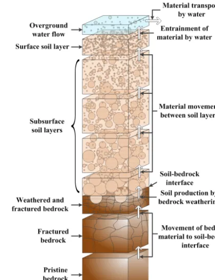
SSSPAM is a state-space matrix model simulating tempo-ral and spatial variation of the grading of the soil profile through depth over a landscape and extends the approach of the mARM model (Cohen et al., 2009) and mARM3D (Cohen et al., 2010). It uses matrix equations to represent physical processes acting upon the soil grading through the soil profile. SSSPAM uses the interaction between a number of layers to simulate soil grading evolution (Fig. 1). These layers are the following: (1) a water layer flowing over the ground which moves soil particles laterally, (2) a surface soil layer from which the water entrains soil particles and which produces an armour over the soil below, (3) several soil lay-ers representing the soil profile, and (4) a semi-infinite non-weathering bedrock/saprolite layer underlying the soil. In SSSPAM two processes are modelled: erosion due to over-land flow, and weathering within the profile. The armouring module consists of three components.
The grading of the surface (armour) layer changes over time because of three competing processes, (1) selective en-trainment of finer fractions by erosion, (2) the resupply of
Figure 1.Schematic diagram of the SSSPAM model (from Cohen et al., 2010).
material from the subsurface (that balances the erosion to ensure mass conservation in the armour layer) and (3) the breakdown of the particles within the armour due to physical weathering. The erosion rate of the armour layer is calcu-lated from the flow shear stress. The entrainment of particles into surface flow at each time step from the armour layer is determined by the erosion transition matrix, which is con-structed using Shield’s shear stress threshold. The Shield’s shear stress threshold determines the maximum particle size that can be entrained in the surface water flow. For particles smaller than the Shield’s shear stress threshold a selective en-trainment mechanism is used which was found to be a good fit to field data (Willgoose and Sharmeen, 2006). Resupply of particles to the armour layer from underneath is mass con-servative. The rate of resupply equals the rate of erosion, so the armour’s mass is constant.
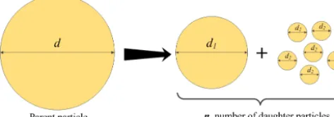
Figure 2. The fragmentation geometry used in SSSPAM (after Wells, et al., 2008).
and one of the cases studied in this paper is a generalisation of this equal volume fragmentation geometry. Weathering in this paper is mass conservative so that when larger particles break into smaller particles the cumulative mass of the soil grading remains constant. Thus we do not model dissolution. The state vectorgdefines the soil grading at any specific time and in every layer. Entriesgi in the state vectorg are the proportion of the material in the grading size range i. The evolution (of the state vector) from one state to another state during a single time step is defined using a matrix equa-tion. This matrix (called the transition matrix) describes the relationship between the states at two times and defines the change in the state during a time step
gt2 =(I+R1t)gt1, (1)
wheregt1 andgt2 are state vectors defining the soil grading at timet1andt2,Ris the marginal transition matrix,Iis the identity matrix, and1tis the timestep (Cohen et al., 2009).
For multiple processes Eq. (1) can be applied sequentially for each process, using theRmatrix appropriate for each of the processes.
Within each layer the equation for weathering follows Eq. (1)
gt2 =[I+(W 1t)B]gt1, (2)
where W is the rate of weathering (which is depth-dependent), and B is the non-dimensional weathering marginal transition matrix. ParameterW determines the rate of weathering whileBdetermines the grading characteristics of the weathered particles.
For the armour layer the mass in the layer is kept con-stant so that as fines are preferentially removed by erosion, the mass removed is balanced by new material added from the layer below, and with the grading of the layer below. For each layer in the profile mass conservation is applied, and any net deficit in mass is (typically) made up from the layer be-low (i.e. by removing material in the layer bebe-low). The only exception to this rule is the case of deposition at the surface where material is pushed down. In this latter case the pushing down results from an excess of mass in the armour layer and this excess propagates down through the profile.
2.1 Constitutive relationships for erosion and armouring The erosion rate (E) of the armour is calculated by a detachment-limited incision model,
E=eq α1Sα2
d50β
a
, (3)
whereeis the erodibility rate,q is discharge per unit width (m3s−1m−1),Sis slope,d50ais the median diameter of the
material in the armour (m),α1,α2 andβare exponents gov-erning the erosion process. It is possible to derive exponents α1 andα2 from the shear stress dependent erosion physics (Willgoose et al., 1991b) or they can be calibrated to field data (e.g. Willgoose and Riley, 1998). In this paper for sim-plicity we will consider a one-dimensional hillslope with a unit width, constant gradient, and a 2 m maximum soil depth. The discharge was calculated by
q=rx, (4)
wherer is the runoff excess generation (m3s−1) and x is the distance down the slope (m) from the slope apex to each node.
The implementation details of the erosion physics (e.g. how selective entrainment of fines is incorporated into the marginal transition matrix for erosion) are identical to that of Cohen et al. (2009) and will not be discussed here. The pri-mary process of relevance here is that a size-selective entrain-ment of fine fractions of the soil grading by erosion is used and it follows the approach of Parker and Klingeman (1982) as calibrated by Willgoose and Sharmeen (2006). The result is that for surfaces that are being eroded the surface becomes coarser with time (and thus why we call the top layer the armour layer).
2.2 Constitutive relationships for weathering
The fracturing geometry determines the weathering transi-tion matrixB. Each grading size class will lose some of its mass to smaller grading size classes as larger parent particles are transformed into smaller daughter particles. The daughter products can fall in one or more smaller grading classes de-pending on the size range of particles produced by the break-down of the larger parent particles. The amount of material received by each smaller size class is a function of size dis-tribution of the grading classes, fracture mechanism, and the size characteristics of the daughter particles.
To generalise the fracture geometries we will assume that a parent particle with a diameterdbreaks into a single daugh-ter particle with diamedaugh-terd1andn−1 smaller daughters with diameterd2(the total number of daughters beingn). For sim-plicity all the particles considered are assumed to be spheri-cal. Mass conservation implies
d3=d13+(n−1)d23. (5)
If the single larger daughter with diameterd1accounts forα fraction of the parent then
d1=α 1
3d (6)
d2= 1−α
n−1 13
d. (7)
By changing theαfraction value and the number of daugh-ters n we are able to simulate various fracture geome-tries such as symmetric fragmentation, asymmetric frag-mentation, and granular disintegration (Wells et al., 2008). For instance α=0.5, n=2 represents symmetric fragmen-tation with two daughter particles, α=0.99, n=11 repre-sents a fracture mechanism resembling granular disintegra-tion where a large daughter retains 99 % of the parent parti-cle volume and 10 smaller daughters have 1 % of the parent volume collectively.
The construction of the weathering transition matrix then follows the methodology outlined in Fig. 1 in Cohen et al. (2009).
2.3 Soil profile development through depth-dependent weathering
The weathering module of SSSPAM consists of two compo-nents. They are (1) the weathering geometry for the grading of the daughter particles discussed above, and (2) the weath-ering rate for the different soil layers which determines the rate at which the parent material is weathered. The weath-ering rate of each soil layer typically (though not always) depends on the depth below the soil surface.
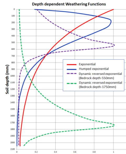
To characterize the weathering rate with soil depth, depth-dependent weathering functions are used. In their mARM3D model Cohen et al. (2010) used two depth-dependent weath-ering functions (Fig. 3), (1) exponential decline (called expo-nential) (Humphreys and Wilkinson, 2007) and (2) humped exponential decline (called humped) (Ahnert, 1977; Minasny and McBratney, 2006). For the exponential, the weathering rate declines exponentially with depth. The rationale under-pinning the exponential function is that the surface soil layer is subjected to the high rates of weathering because it is closer to the surface where wetting and drying, and temper-ature fluctuations are greatest. The humped function has the maximum weathering rate at a finite depth below the surface
Figure 3. Graphical representation of all the depth-dependent weathering functions used in SSSPAM.
instead of being at the surface itself and then declines ex-ponentially below that depth. The rationale for the humped function is evidence that the weathering is highest at the wa-ter table surface which leads to a humped function.
The three depth-dependent weathering functions are graphically represented by Fig. 3. The exponential function is (Cohen et al., 2010)
wh=β0e(−δ1h), (8)
wherewh is the weathering rate at the soil layer at a depth ofh(m) below the surface andδ1is the depth scaling factor (hereδ1=1.738).
The humped function used is (Minasny and McBratney, 2006)
wh=
P0e(−δ2h+Pa)−e(−δ3h)
M , (9)
whereP0andPaare the maximum weathering rate and the steady state weathering rate respectively,δ2andδ3are con-stants used to characterise the shape of the function, andM is the maximum weathering rate at the hump which is used to normalise the function. Values we used here wereP0=0.25, Pa=0.02,δ2=4,δ3=6, andM=0.04.
The dynamic reversed exponential function is
wh=
1−λ1−e−δ4(H−h) for h≤H
1−λ1−e−δ5(h−H) for h > H , (10)
whereH is the depth (m) to the soil bedrock interface from the surface which is calculated from the soil grading distri-bution at each iteration during the simulation,λis a constant which determines the function value at the asymptote,δ4and δ5are constants used to characterise the rate of decline with depth of the function. We usedλ=0.98,δ4=3,δ5=10.
The non-zero weathering below the bedrock-soil interface in Eq. (10) represents a slower rate of chemical weathering within the bedrock due to its lower porosity and hydraulic conductivity. In generalδ5>δ4.
The weathering rate of each layer is determined by mod-ifying the base weathering rate W0 (Eq. 2) and the depth-dependent weathering function used,f(h). The weathering rate of a soil layer at a depth ofhfrom surfaceWh is given by
Wh=W0f(h). (11)
3 Data used in this study
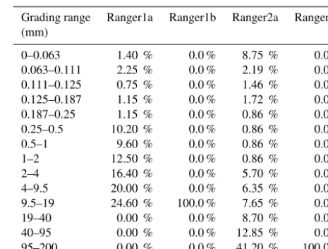
Four soil particle size distribution data sets were used as in-put data for SSSPAM simulations. Two particle size distri-bution data sets were collected from the Ranger Uranium Mine (Northern Territory, Australia) spoil site (Willgoose and Riley, 1998; Sharmeen and Willgoose, 2007; Cohen et al., 2009; Coulthard et al., 2012). The third and fourth grad-ings were created from the previous two gradgrad-ings to simulate the subsurface bedrock conditions. The naming convention used here is “a” for the actual grading data set and “b” for the
Table 1.Size distribution of soil gradings used for SSSPAM4D simulation.
Grading range Ranger1a Ranger1b Ranger2a Ranger2b (mm)
0–0.063 1.40 % 0.0 % 8.75 % 0.0 %
0.063–0.111 2.25 % 0.0 % 2.19 % 0.0 %
0.111–0.125 0.75 % 0.0 % 1.46 % 0.0 %
0.125–0.187 1.15 % 0.0 % 1.72 % 0.0 %
0.187–0.25 1.15 % 0.0 % 0.86 % 0.0 %
0.25–0.5 10.20 % 0.0 % 0.86 % 0.0 %
0.5–1 9.60 % 0.0 % 0.86 % 0.0 %
1–2 12.50 % 0.0 % 0.86 % 0.0 %
2–4 16.40 % 0.0 % 5.70 % 0.0 %
4–9.5 20.00 % 0.0 % 6.35 % 0.0 %
9.5–19 24.60 % 100.0 % 7.65 % 0.0 %
19–40 0.00 % 0.0 % 8.70 % 0.0 %
40–95 0.00 % 0.0 % 12.85 % 0.0 %
95–200 0.00 % 0.0 % 41.20 % 100.0 %
synthetic bedrock corresponding to the actual data set (e.g. Ranger1a is the actual data set and Ranger1b is the synthetic bedrock corresponding to Ranger1a actual data set). Further details are given below (Table 1).
– Ranger1a: this grading distribution was first used by Willgoose and Riley (1998) for their landform evolu-tion modelling experiments. This soil grading was sub-sequently used by Sharmeen and Willgoose (2007) and Cohen et al. (2009) for their armouring and weathering simulations. This grading distribution consists of stony metamorphic rocks of medium to coarse size produced by mechanical weathering breakdown, has a median di-ameter of about 3.5 mm, and has a maximum didi-ameter of 19 mm.
– Ranger2a: the second grading distribution was used by Coulthard et al. (2012) in their soil erosion modelling experiments and has a maximum diameter of 200 mm. The Coulthard data set includes a coarse fraction which is not included in Ranger1a, has a median diameter of 40 mm, and has a maximum diameter of 200 mm. Nom-inally Gradings 1a and 2a are for the same site but the gradings are not identical in the overlapping part of the grading below 19 mm.
– Ranger1b and Ranger2b: these grading data sets were created using the particle distribution classes of Ranger1a and Ranger2a to represent the underlying bedrock for each of the grading distributions mentioned above. To represent the bedrock for these data sets 100 % of the material was assumed to be in the largest diameter class for each grading classes (19 mm for the 1b and 200 mm for 2b).
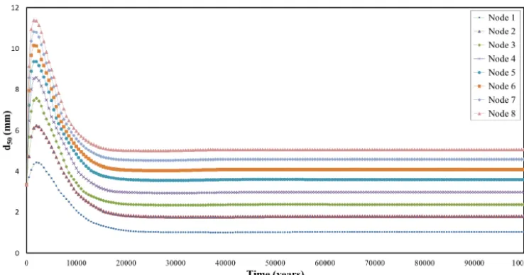
Figure 4.d50Evolution of the nodes with lowest slope gradient (2.1 %).
represented by 21 layers representing the armour layer and 20 subsurface layers. Initially the armour layer was set to ei-ther Ranger1a or Ranger2a grading data set (depending on the type of simulation) and all the subsurface layers were set to the corresponding bedrock layer (for Ranger1a sur-face grading Ranger1b was set as the bedrock grading for all other subsurface layers). For brevity henceforth simulations run with the “Ranger1 data set” used the Ranger1a grading for the initial surface layer and Ranger1b as the subsurface grading unless otherwise stated. Likewise “Ranger2 data set” means, Ranger2a for the initial surface and Ranger2b for the subsurface). We have used 30 years of measured pluviograph data (Willgoose and Riley, 1998) to calculate discharge. The 30 years of runoff was repeated to create a 100-year data set as was done in our earlier work (Sharmeen and Willgoose, 2006; Cohen et al., 2009).
4 SSSPAM calibration
To provide a realistic nominal parameter set around which parameters could be varied in the parametric study, SSSPAM was calibrated to mARM3D, which in turn had been cali-brated to ARMOUR1D (Willgoose and Sharmeen, 2006) and we know ARMOUR1D corresponded well with field data.
Figure 5 shows a comparison between contour plots gener-ated by mARM3D and SSSPAM using identical initial con-ditions (Ranger1 data set) and model parameters. The figure shows that mARM3D and SSSPAM produce similard50 val-ues, though SSSPAM is very slightly coarser. The slight dif-ferences between the two contour plots result from the im-proved numerics of SSSPAM and an imim-proved implemen-tation of the matrix methodology in SSSPAM. We are thus confident that SSSPAM and mARM3D are comparable. The parameter values used for SSSPAM areα1=1.0,α2=1.2, β=1.0,m=4,e=2.5×10⁻⁸andn=0.1.
Figure 5.Log-log Area-Slope-d50 contour plots generated using the Ranger1 data set.(a)mARM3D (Cohen et al., 2009),(b) SSS-PAM. The dotted lines in(b)are hypothetical long profiles down a drainage line showing how the contour figure can be used to gener-ate soil properties down a drainage line. See the text for more detail.
5 SSSPAM simulations and results
Cohen et al. (2009, 2010) found a strong log-log linear re-lationship between contributing area, slope and the d50 of the armour soil grading. They quantified the relationship be-tween soil grading, local topographic gradient and drainage area by
AαS
d50ε =constant, (12)
(i.e. median) of the soil grading, andαandεare constants. Cohen used only one parent material grading and one param-eter set for his analyses. To explore the generality of Eq. (12), we have examined the behaviour of the contour plots with changes to (1) weathering parameters, (2) grading of the pent material, (3) process and climate parameters, and (4) ar-mouring mechanisms. We also examined a broader range of area-slope combinations that would typically occur in na-ture (since we are interested in man-made landforms which may have far from natural geomorphology), and which Co-hen examined. For the initial conditions, unless otherwise indicated, in each simulation the “a” grading was used for the initial surface layer and the corresponding “b” bedrock grading for all the initial subsurface layers (e.g. Ranger1a for the surface and Ranger1b for the subsurface). To ensure that the hillslopes had reached equilibrium, the model simulated 100 000 years with output every 200 years. Equilibrium was assessed to occur when the grading of all nodes on the hill-slope stopped changing, typically well before 100 000 years. Figure 4 shows a time seriesd50 evolution of all the nodes with lowest slope gradient (2.1 %). It shows that equilibrium is reached well before 100 000 years. Hillslopes with higher gradients reached equilibrium even faster.
5.1 Interpretation of the grading contour plots
Before discussing the parametric study and its myriad of con-tour plots, Fig. 5 shows how the concon-tour plots can be used to estimate soil properties for any hillslope type. Five profiles are illustrated:
Curve 1: This is a hillslope where the slope is increasing down the hillslope so is concave down in profile and looks like a rounded hilltop. Thed50increases down the hillslope (i.e. increasing area, moving from left to right in Fig. 5). All our contour plots increase from left to right and from bottom to top, so in general concave hill-slopes will always coarsen downslope.
Curve 2: This hillslope has constant slope downslope and, as for slope 1, will always coarsen downslope.
Curve 3: This hillslope has slopes that are decreasing downslope and is concave up. Importantly the gradient of the line in Fig. 5 is less than the gradient of the con-tours so the hillslope coarsens downslope.
Curve 4: This hillslope is similar to 3 except that the rate of decrease of slope downstream is more severe (i.e. con-cavity is greater) so the gradient of the line in Fig. 5 is steeper than the gradient of the contours. This hillslope fines downstream.
Curve 5: This hillslope is a classic catena profile with a rounded hilltop and a concave profile downstream of the hilltop. By tracking this hillslope downstream the sur-face grading (or sursur-faced50) will initially coarsen. As
it transitions to concave up it will continue to coarsen until the rate of reduction of the hillslope slope is severe enough that is starts to fine downstream. Whether this latter region of fining occurs will depend on the con-cavity of the hillslope and whether it is strong enough relative to the gradient of the soil contours in Fig. 5.
Note that the erosion model in SSSPAM is an incision model dependent on upstream area and slope. With this model the planar shape and slopes of the catchment up-stream of the point are irrelevant, so while we derived Fig. 5 for a planar hillslope it is equally valid for a natural two-dimensional catchment with flow divergence and conver-gence. Thus it should be clear that the spatial distribution of soils, and any questions of downslope fining or coarsening of those soils, must depend on the interaction between the pe-dogenesis processes that produce the soils (and thus drive the area-slope dependence of soil grading) and landform evolu-tion processes that generate those profiles (and the area-slope relations for those slopes). Ultimately deeper understanding of these links will only come from a coupled landscape-soilscape evolution model, but in this paper we confine our-selves to better understanding of the soilscape processes and the area-slope dependence of grading. The coupled model will be discussed in a subsequent paper.
5.2 Parametric Study of SSSPAM
All the nominal parameters used in the parametric study are presented in Table 2. In order to fully explore the area-slope-d50 relationship a parametric study was carried out using SSSPAM. The area-slope-diameter relationship was derived by evolving the soil on a number of one-dimensional, con-stant width, planar hillslopes, each with a different slope, with evolution continuing until the soil reached equilibrium. A contour plot was then created where the soil grading met-ric (usually the median diameter, d50) was contoured for a range of slopes and area. Because of the planar slope, only erosion occurs, no deposition. Erosion is a function of local discharge, slope and soil surface grading as indi-cated in Eq. (3), and is assumed to be detachment-limited. Detachment-limitation means that the upstream sediment loads do not impact on erosion rates. Hillslope elevations are not evolved (i.e. no landform evolution occurs) which is equivalent to assuming that the soil evolves more rapidly than the hillslope so that the soils equilibrate quickly to any landform changes.
5.2.1 Changing surface and subsurface gradings and weathering rate
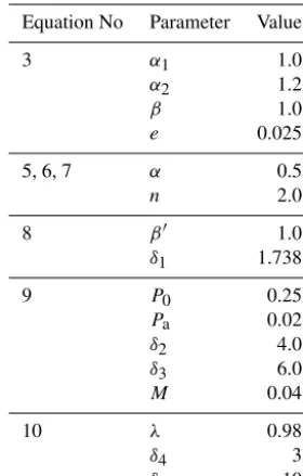
Table 2.Parameters used in the simulations generate Fig. 6a2.
Equation No Parameter Value
3 α1 1.0
α2 1.2
β 1.0
e 0.025
5, 6, 7 α 0.5
n 2.0
8 β0 1.0
δ1 1.738
9 P0 0.25
Pa 0.02
δ2 4.0
δ3 6.0
M 0.04
10 λ 0.98
δ4 3
δ5 10
Figure 7. Equilibrium contour plots ofd50 generated using the Ranger1 data set with identical model parameters as used in Fig. 6a2 except changing the runoff rate, half the nominal runoff rate.
if the initial surface grading was changed. For example, using the Ranger1a or Ranger2b grading data for the surface but with Ranger2b for the bedrock yielded identical equilibrium d50results. As weathering broke down the surface layer and it was eroded it was replaced by the weathered bedrock ma-terial, which was identical when the same subsurface grading and weathering mechanism was used. Finally a coarser sub-surface grading led to a coarser armour.
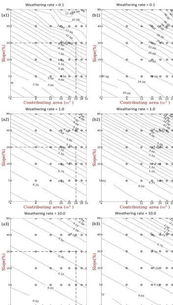
These trends with weathering rate are consistent with Co-hen et al. (2010) where the log-log linear area-slope-d50 re-lationship was observed regardless of the weathering rate. Moreover the contour lines in Fig. 6 all have the same slope. This implies that although the magnitude of the coarseness of the equilibrium armour depends on the underlying soil grad-ing and weathergrad-ing mechanism, the slope of the contours is independent of the subsurface grading and weathering pro-cess. This result demonstrates that the area-slope-d50 rela-tionship is robust against changes in the grading of the source material, and the only change is in the absolute grading, not the grading trend with area and slope.
5.2.2 Changing the runoff rate
Erosion is a function of the discharge, and the discharge de-pends on the climate and rainfall. The effect of changing the runoff is shown in Fig. 7. To simulate a more arid climate the runoff generation parameter in Eq. (4) was halved. Fig-ure 7 shows that a reduced discharge produced a finer armour. While not shown, higher discharge rates produced coarser ar-mour. For lower discharges (1) the Shield’s Stress threshold decreases thus allowing smaller particles to be retained in the armour layer, and (2) the rate of erosion decreases while the weathering rate remains constant so that weathering (i.e. fin-ing) becomes more dominant. Both of these processes work in tandem to produce finer armour. This conclusion is qual-itatively consistent with Cohen et al. (2013), where they ap-plied natural climate variability over several ice-age cycles and observed switching between fining and coarsening of the soil surface depending on the relative dominance of erosion and weathering at different stages in the climate cycle.
5.2.3 Changing the erosion discharge and slope exponents
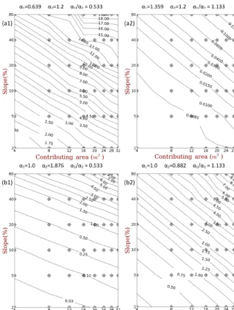
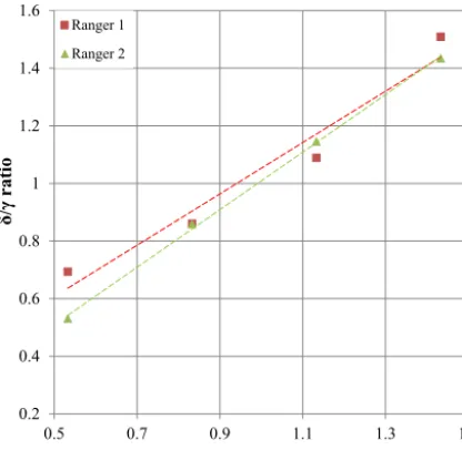
The influence of the exponents on area and slope in the ero-sion equation (Eq. 3),α1andα2, is shown in Fig. 8. These contour plots used the Ranger1a surface grading for the sur-face grading and Ranger1b bedrock grading for the initial subsurface layers. Figure 8 shows that although thed50 val-ues changed with differentα1andα2values, the slope of the contours only changed whenα1/α2was changed. To inves-tigate the generality of this conclusion, contours were then plotted for different α1/α2. The slope of the contours was strongly correlated withα1/α2. The slope of the contours in-creased for higherα1/α2ratios. Similar results were obtained for the Ranger2 data set. Theα1/α2ratio not only influences the slope of the contour lines but also influences the equilib-riumd50 values. For lowα1/α2, the equilibriumd50 values at the hillslope nodes were coarser than for highα1/α2.
These relationships allow us to generalise the area-slope-d50relationship
d50= cAδSγ 1/ε
Figure 8.Equilibrium contour plots ofd50 generated using Ranger1 data set with identical model parameters as Fig. 6a2 (i.e.α1=1.0,
α2=1.2,α1/α2=0.833) except changingα1andα2values generated using(a1, b1)differentα1and constantα2values,(a2 b2)different
α2and constantα1values.
whereδ,γ andεare exponents on contributing area, slope andd50 respectively, andcis a constant, and where the ra-tioδ/γ is a function of the erosion dependence on area and slope.
Figure 9 shows thatδ/γ was strongly correlated with the modelα1/α2even though there was no correlation with the individual parameters (i.e. α1withδ, orα2 withγ). In the regression analysis the parameterεwas assumed to be 1 in order to calculate δ andγ constants. This assumption does not affect theδ/γ ratio. This result was independent of the subsurface grading.
5.2.4 Changing the erodibility and selectivity exponent
βande
0.2 0.4 0.6 0.8 1 1.2 1.4 1.6
0.5 0.7 0.9 1.1 1.3 1.5
δ/
γ
rati
o
Model α1/α2 ratio
Ranger 1 Ranger 2
Figure 9.Correlation between the modelα1/α2andδ/γ.
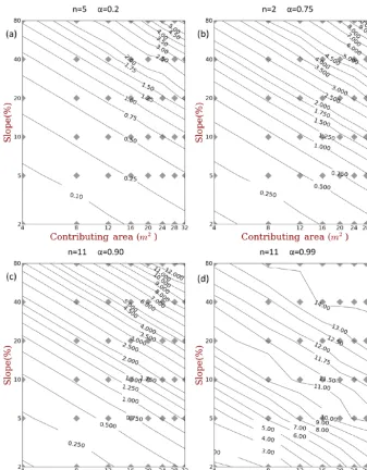
5.2.5 Different weathering fragmentation geometries To study different weathering mechanisms we used a frag-mentation geometry (Fig. 2) that has two parameters, n and α (Eqs. 5–7). The simulations in the previous sec-tions used symmetric fragmentation withn=2 andα=0.5 (i.e. where a parent particle breaks down to two equal vol-ume daughter particles). Here we examine four other ge-ometries, (1) symmetric fragmentation with multiple daugh-ter products (n=5,α=0.2; i.e. the parent breaks into five equal daughters each having 20 % of the volume of the par-ent), (2) moderately asymmetric (n=2,α=0.75; the ent breaks into two daughters, with 75 and 25 % of the par-ent volume), (3) granular disintegration (n=11,α=0.9; the parent breaks into 11 daughters, one with 90 % of the parent volume and the other 10 daughters each have 1 % of the par-ent volume), and (4) as for Geometry 3 but with the large daughter having 99 % of the parent particle volume (n=11, α=0.99). Figure 10 shows results using the Ranger1 data set. The corresponding symmetric results are in Fig. 6. Sym-metric fragmentation with five equal daughter particles (Ge-ometry 1) leads to the finest equilibrium contour plot but the contours are otherwise unchanged. The granular disintegra-tion geometries produced coarser results with the coarsest ar-mour from Geometry 4. We conclude that when fragmenta-tion produces a number of symmetric daughters the equilib-rium grading of a hillslope is finest. Finally the slope of the contours did not change for different fragmentation geome-tries.
5.2.6 Effect of initial conditions
The simulations in the sections above used the same grad-ing for the initial surface and the subsurface. To explore the
initial conditions we changed the initial surface and subsur-face data sets. The equilibrium grading contour plot gener-ated using Ranger2a surface grading and Ranger1b subsur-face gradings was identical to the equilibrium grading con-tour plot generated using Ranger1a surface and Ranger1b subsurface grading. Likewise the equilibrium grading con-tour plot generated using Ranger1a surface and Ranger2b subsurface gradings was identical to the equilibrium grading contour plot generated using Ranger2a surface and Ranger2b for subsurface gradings. The results were slightly different for different subsurface gradings. These results also show that, as expected, there was no effect of the initial conditions on the equilibrium grading. Though not shown the influence of the initial grading is only felt during the dynamic phase of the simulation before the armour reaches equilibrium.
5.3 Generalising beyond median grain size
The results above have focussed ond50as a measure of soil grading. However, the model can provide any particle per-centile or statistic of interest. Figure 11 shows area-slope re-sults ford10(i.e. 10 % by mass is smaller than this diameter). It shows that the general trends observed in thed50contour plots (Fig. 6b2) are also evident ind10. Though not shown, similar results were found ford90. The slope of the contours is independent of diameter but as expected thed10 andd90 values are rankedd10<d50<d90. We conclude that the area-slope-diameter relationship we have observed in our simula-tions is robust across the grading profile.
5.4 Influence of the depth-dependent weathering functions
In this section we consider the three different depth-dependent weathering functions (Fig. 3, Eqs. 8 to 10) for the weathering rate in the subsurface soil layers. All the simu-lations in the previous sections used the exponential func-tion (Eq. 8). Figures 5 and 12 show that the contour plots for all weathering functions are very similar. However, as slope and area are increased the humped function produces a more rapidly coarsening armour. Overall the reversed nential produces the coarsest armour. For the reversed expo-nential after an initially high weathering rate at the surface, the weathering rate reduces rapidly as the soil-bedrock inter-face moves deeper into the soil profile. This low near surinter-face weathering decreases the rate of fining of the armour and dra-matically reduces the erosion. This reduction in erosion rate prevents weathered fine particles from reaching the surface.
Figure 10.Equilibrium contour plots of d50 generated using Ranger1 data set with identical model parameters as Fig. 6a2 (i.e.n=2,
α=0.5; symmetric fragmentation with 2 daughter particles) with different weathering geometries (n=number of daughter particles andα= material fraction retained by largest daughter particle)(a)symmetric fragmentation withn=5 andα=0.2(b)asymmetric fragmentation withn=2 andα=0.75(c)granular disintegration withn=11 andα=0.9,(d)granular disintegration withn=11 andα=0.99.
the humped function produces a shallower soil and a coarser armour compared with the exponential. In contrast, the re-versed exponential produces a markedly different soil profile. It produces very coarse armour, a soil thickness beyond the modelled 2000 mm limit, and a more uniform soil grading through the profile. This latter result is because the weath-ering is greatest at the bedrock-soil interface so most of the soil grading change is focussed at the base of the profile and relatively less occurs within the profile.
A final question is whether the area-slope-grading rela-tionship occurs only in the armour or exists throughout the profile using the exponential weathering function. We
weath-Figure 11. Equilibrium contour plots of d10 generated using Ranger1 data set with identical model parameters as Fig. 6a2 (where thed50results are presented).
Figure 12. Equilibrium contour plots of d50 generated using Ranger1 data set with identical model parameters as Fig. 6a2 except changing the depth-dependent weathering function to(a)humped,
(b)dynamic reversed exponential.
ering function, couples the spatial organisation of the sur-face with the spatial organisation of the soil profile at depth. Therefore what happens at the surface affects the entire pro-file.
6 Discussion
Here we have used a new pedogenesis model, SSSPAM, to analyse the equilibrium soil grading and spatial organisation of soil profiles. This model extends the mARM3D model of Cohen et al. (2010) and improves the numerics. Our results have generalised previous studies (Cohen et al., 2009, 2010, 2013) that have found a log-log linear relationship between
d50, contributing area and slope. Using a broader range of environmental conditions, we have found that log-log linear relationship for grading is robust against changes in envi-ronment and underlying geology and for hillslopes where the dominant processes are surface fluvial erosion and in-profile weathering. The main factors influencing the quan-titative form of the relationship are the area and slope depen-dency of the erosion equation, and the relative rates of the weathering and erosion processes. Coarsening of the downs-lope nodes was observed in all the simulations.
Our parametric study has demonstrated the versatility of our model for studying the influence of different process pa-rameters and the dynamics of hillslope evolution. Our d10 andd90contour plots show that the area-slope-diameter rela-tionship is not only true ford50 but is also true for other as-pects of the particle size grading of the soil. This strengthens our confidence in the generality of the area-slope-diameter relationship. This relationship provides us with a methodol-ogy to predict the characteristics of soil grading on a hill-slope as a function of geomorphology. It also allows us to interpolate between field measurements. Furthermore, our parametric study showed how parameters of the armouring component affect the area-slope-diameter relationship. Par-ticularly interesting was that the ratio of the erosion expo-nents (α1/α2) changes the slope of the contours. This obser-vation also hints at the importance of topographic and pro-cess characteristics in soil evolution and hillslope catena and how these topographical units may be used for predictive soil mapping and inference of erosion process.
Previous work (e.g. Willgoose, et al., 1991b; Tucker and Whipple, 2002) has shown that topography is also a func-tion ofα1/α2and this suggests a strong underlying process link between the spatial distribution of topography and the spatial distribution of soil grading that goes beyond the con-cept of soil catena. The soil catena concon-cept says that sys-tematic changes occur in soils as a function of their position on the hillslope. Our results suggest that the same processes that influence the equilibrium distribution of topography (e.g. the erosion process that determinesα1/α2) also influence the equilibrium distribution of soils. Thus while a soil catena pre-sumes a causal link from topography, we postulate a causal link for both topography and soils from erosion processes.
Using our model we were able to explore the soil profile characteristics and how the soil profile will change depend-ing on the weatherdepend-ing characteristics of the bedrock material. Another important insight is that the area-slope-d50 relation-ship is present in all the subsurface layers as well as the sur-face armour.
weather-Figure 13.Equilibrium soil profiled50 generated using the Ranger1 data set with a one-dimensional hillslope with 10 % slope and 32 m length using(a)exponential,(b)humped,(c)reversed exponential weathering functions.
ing mechanisms to predict the equilibrium soil distribution of hillslopes. There is a need to explicitly incorporate chemi-cal and biologichemi-cal weathering (Green et al., 2006; Lin, 2011; Riebe et al., 2004; Roering et al., 2002; Vanwalleghem et al., 2013). Another important aspect needed is accounting for deposition of sediments so that we can model alluvial soils which requires a transport-limited erosion model. A fu-ture task is to incorporate a soils model like SSSPAM into a landform evolution model such as SIBERIA (Willgoose et al., 1991a). This would allow the modelling of the interaction between the pedogenesis process in this paper with hillslope transport processes such as creep and bioturbation. If soils evolve rapidly then it may be possible to use the equilibrium grading results from this paper as the soilscape model, on the basis that the soil evolves fast enough to always be at, or near, equilibrium with the evolving landform. If soils evolve slowly then it may be necessary to fully couple the soils and landform evolution models. This is a subtle, and not fully
re-solved, question of relative response times of the soils and the landforms (Willgoose et al., 2012).
7 Conclusions
Figure 14.Equilibrium contour plots ofd50generated using the Ranger1 data set with identical model parameters as used in Fig. 6a2 for different subsurface soil layers(a)layer 1 (100 mm depth),(b)layer 5 (500 mm depth),(c)layer 10 (1000 mm depth),(b)layer 15 (1500 mm depth).
how this relationship would change with changes in the pe-dogenic processes. We found that the ratio of the erosion ex-ponents on discharge and slope,α1/α2, changes the angle of the contours in the log-log contour plots (Fig. 7). This has application in the field of digital soil mapping where easily measurable topographical properties can be used to predict the characteristics of soil properties. Importantly, the con-tributing area and the slope data can be easily derived from a digital elevation model, which can be produced using re-mote sensing and GIS techniques. Coupling SSSPAM with a GIS system can potentially improve the field of digital soil mapping by providing a physical basis to existing empirical methods and potentially streamlining existing resource
inten-sive and time-consuming soil mapping techniques as, for ex-ample, in the current initiatives in global digital soil mapping (Sanchez et al., 2009).
SSSPAM has the potential to be a powerful tool for under-standing and modelling pedogenesis and its morphological implications.
8 Data availability
The data and codes used in this paper can be obtained by contacting the authors.
Acknowledgements. This work was supported by Australian Research Council Discovery Grant DP110101216. The SSSPAM model and the parameters used in this paper are available on request from the authors.
Edited by: V. Vanacker
References
Ahnert, F.: Some comments on the quantitative formulation of ge-omorphological processes in a theoretical model, Earth Surface Proc. Land., 2, 191–201, doi:10.1002/esp.3290020211, 1977. Anderson, R. S. and Anderson, S. P.: Geomorphology: The
Me-chanics and Chemistry of Landscapes, Cambridge Press, Cam-bridge, ISBN-13: 978 0 521 51978 6, 2010.
Behrens, T. and Scholten, T.: Digital soil mapping in Ger-many – a review, J. Plant Nutr. Soil Sc., 169, 434–443, doi:10.1002/jpln.200521962, 2006.
Benites, V. M., Machado, P. L. O. A., Fidalgo, E. C. C., Coelho, M. R., and Madari, B. E.: Pedotransfer functions for estimating soil bulk density from existing soil survey reports in Brazil, Geo-derma, 139, 90–97, doi:10.1016/j.geoderma.2007.01.005, 2007. Braun, J., Heimsath, A. M., and Chappell, J.: Sediment transport mechanisms on soil-mantled hillslopes, Geology, 29, 683–686, 2001.
Bryan, R. B.: Soil erodibility and processes of water erosion on hillslope, Geomorphology, 32, 385–415, doi:10.1016/S0169-555X(99)00105-1, 2000.
Cohen, S., Willgoose, G., and Hancock, G.: The mARM spa-tially distributed soil evolution model: A computationally ef-ficient modeling framework and analysis of hillslope soil sur-face organization, J. Geophys. Res.-Earth Surf., 114, F03001, doi:10.1029/2008jf001214, 2009.
Cohen, S., Willgoose, G., and Hancock, G.: The mARM3D spatially distributed soil evolution model: Three-dimensional model framework and analysis of hillslope and landform responses, J. Geophys. Res.-Earth Surf., 115, F04013, doi:10.1029/2009jf001536, 2010.
Cohen, S., Willgoose, G., and Hancock, G.: Soil-landscape response to mid and late Quaternary climate fluctuations based on numerical simulations, Quat. Res., 79, 452–457, doi:10.1016/j.yqres.2013.01.001, 2013.
Coulthard, T. J., Hancock, G. R., and Lowry, J. B. C.: Modelling soil erosion with a downscaled landscape evolution model, Earth Surf. Proc. Land., 37, 1046–1055, doi:10.1002/esp.3226, 2012. Gessler, J.: Self-stabilizing tendencies of alluvial channels, J.
Wa-terway. Div-ASCE, 96, 235–249, 1970.
Gessler, P. E., Moore, I., McKenzie, N., and Ryan, P.: Soil-landscape modelling and spatial prediction of soil attributes, Int. J. Geogr. Inf. Syst., 9, 421–432, 1995.
Gessler, P., Chadwick, O., Chamran, F., Althouse, L., and Holmes, K.: Modeling soil–landscape and ecosystem properties using ter-rain attributes, Soil Sci. Soc. Am. J., 64, 2046–2056, 2000. Gomez, B.: Temporal variations in bedload transport rates: The
ef-fect of progressive bed armouring, Earth Surf. Proc. Land., 8, 41–54, doi:10.1002/esp.3290080105, 1983.
Govers, G., Van Oost, K., and Poesen, J.: Responses of a semi-arid landscape to human disturbance: a simulation study of the inter-action between rock fragment cover, soil erosion and land use change, Geoderma, 133, 19–31, 2006.
Green, E. G., Dietrich, W. E., and Banfield, J. F.: Quan-tification of chemical weathering rates across an actively eroding hillslope, Earth Planet. Sc. Lett., 242, 155–169, doi:10.1016/j.epsl.2005.11.039, 2006.
Hillel, D.: Introduction to soil physics, Academic Press, London, 364 pp., 1982.
Humphreys, G. S. and Wilkinson, M. T.: The soil production func-tion: A brief history and its rediscovery, Geoderma, 139, 73–78, doi:10.1016/j.geoderma.2007.01.004, 2007.
Jenny, H.: Factors of soil formation, McGraw-Hill Book Company New York, NY, USA, 191 pp., ISBN-10: 0-486-68128-9, 1941. Lin, H.: Three Principles of Soil Change and Pedogenesis in
Time and Space, Soil Sci. Soc. Am. J., 75, 2049–2070, doi:10.2136/sssaj2011.0130, 2011.
Lisle, T. and Madej, M.: Spatial variation in armouring in a channel with high sediment supply, in: Dynamics of gravel-bed rivers, edited by: Billi, P., Thorne, C. R., and Tacconi P., John Wiley, New York, 277–293, 1992.
Little, W. C. and Mayer, P. G.: Stability of channel beds by armor-ing, J. Hydr. Eng. Div.-ASCE, 102, 1647–1661, 1976.
McBratney, A. B., Mendonça Santos, M. L., and Minasny, B.: On digital soil mapping, Geoderma, 117, 3–52, doi:10.1016/S0016-7061(03)00223-4, 2003.
Minasny, B. and McBratney, A. B.: Mechanistic soil-landscape modelling as an approach to developing pe-dogenetic classifications, Geoderma, 133, 138–149, doi:10.1016/j.geoderma.2006.03.042, 2006.
Moore, I. D., Gessler, P. E., Nielsen, G. A., and Pe-terson, G. A.: Soil Attribute Prediction Using Ter-rain Analysis, Soil Sci. Soc. Am. J., 57, 443–452, doi:10.2136/sssaj1993.03615995005700020026x, 1993. Ollier, C.: Weathering, Longman group, London, 270 pp., 1984. Ollier, C. and Pain, C.: Regolith, soils and landforms, John Wiley &
Sons, Chichester, 316 pp., 1996.
Parker, G. and Klingeman, P. C.: On why gravel bed streams are paved, Water Resour. Res., 18, 1409–1423, doi:10.1029/WR018i005p01409, 1982.
Poesen, J. W., van Wesemael, B., Bunte, K., and Benet, A. S.: Vari-ation of rock fragment cover and size along semiarid hillslopes: a case-study from southeast Spain, Geomorphology, 23, 323–335, 1998.
Roering, J. J., Almond, P., Tonkin, P., and McKean, J.: Soil trans-port driven by biological processes over millennial time scales, Geology, 30, 1115–1118, 2002.
Roering, J. J., Perron, J. T., and Kirchner, J. W.: Functional rela-tionships between denudation and hillslope form and relief, Earth Planet. Sc. Lett., 264, 245–258, 2007.
Sanchez, P. A., S., Ahamed, F., Carré, A. E., Hartemink, J., Hempel, J., Huising, P., Lagacherie, A. B., McBratney, N. J., McKenzie, and de Lourdes, M.: Mendonça-Santos, Digital soil map of the world, Science, 325, 680–681, 2009.
Scull, P., Franklin, J., Chadwick, O., and McArthur, D.: Predictive soil mapping: a review, Prog. Phys. Geog., 27, 171–197, 2003. Sharmeen, S. and Willgoose, G. R.: The interaction between
ar-mouring and particle weathering for eroding landscapes, Earth Surf. Proc. Land., 31, 1195–1210, doi:10.1002/esp.1397, 2006. Sharmeen, S. and Willgoose, G. R.: A one-dimensional model
for simulating armouring and erosion on hillslopes: 2. Long term erosion and armouring predictions for two contrast-ing mine spoils, Earth Surf. Proc. Land., 32, 1437–1453, doi:10.1002/esp.1482, 2007.
Singh, V. and Woolhiser, D.: Mathematical Modeling of Watershed Hydrology, J. Hydrol. Eng., 7, 270–292, doi:10.1061/(ASCE)1084-0699(2002)7:4(270), 2002.
Strahler, A. H. and Strahler, A. N.: Introducing physical geography, 4th ed. Hoboken, NJ, John Wiley, ISBN-10: 047167950X, 2006. Thornbury, W. D.: Principles of geomorphology, Wiley New York,
ISBN-10: 0471861979, 594 pp., 1969.
Triantafilis, J., Gibbs, I., and Earl, N.: Digital soil pattern recog-nition in the lower Namoi valley using numerical clustering of gamma-ray spectrometry data, Geoderma, 192, 407–421, doi:10.1016/j.geoderma.2012.08.021, 2013.
Tucker, G. E. and Whipple, K. X.: Topographic outcomes pre-dicted by stream erosion models: Sensitivity analysis and intermodel comparison, J. Geophys. Res.-Solid, 107, 2179, doi:10.1029/2001JB000162, 2002.
Vanwalleghem, T., Stockmann, U., Minasny, B., and McBratney, A. B.: A quantitative model for integrating landscape evolu-tion and soil formaevolu-tion, J. Geophys. Res.-Earth, 118, 331–347, doi:10.1029/2011JF002296, 2013.
Wells, T., Binning, P., Willgoose, G., and Hancock, G.: Laboratory simulation of the salt weathering of schist: I. Weathering of schist blocks in a seasonally wet tropical environment, Earth Surf. Proc. Land., 31, 339–354, doi:10.1002/esp.1248, 2006.
Wells, T., Willgoose, G. R., and Hancock, G. R.: Modeling ering pathways and processes of the fragmentation of salt weath-ered quartz-chlorite schist, J. Geophys. Res.-Earth Surf., 113, F01014, doi:10.1029/2006jf000714, 2008.
West, N., Kirby, E., Bierman, P., and Clarke, B. A.: Aspect-dependent variations in regolith creep revealed by meteoric 10Be, Geology, 42, 507–510, 2014.
Wilford, J.: A weathering intensity index for the Australian continent using airborne gamma-ray spectrometry and digital terrain analysis, Geoderma, 183–184, 124–142, doi:10.1016/j.geoderma.2010.12.022, 2012.
Willgoose, G. R.: Modeling Soilscape and Landscape Evolution, Cambridge Press, Cambridge, in press, 2017.
Willgoose, G. R. and Sharmeen, S.: A One-dimensional model for simulating armouring and erosion on hillslopes: I. Model devel-opment and event-scale dynamics, Earth Surf. Process. Landf., 31, 970–991, doi:10.1002/esp.1398, 2006.
Willgoose, G. and Riley, S.: The long-term stability of engi-neered landforms of the Ranger Uranium Mine, Northern Ter-ritory, Australia: Application of a catchment evolution model, Earth Surf. Proc. Land., 23, 237–259, doi:10.1002/(sici)1096-9837(199803)23:3<237::aid-esp846>3.0.co;2-x, 1998.
Willgoose, G., Bras, R. L., and Rodriguez-Iturbe, I.: A coupled channel network growth and hillslope evolution model: 1. Theory, Water Resour. Res., 27, 1671–1684, doi:10.1029/91wr00935, 1991a.
Willgoose, G., Bras, R. L., and Rodriguez-Iturbe, I.: A physical ex-planation of an observed link area-slope relationship, Water Re-sour. Res., 27, 1697–1702, doi:10.1029/91wr00937, 1991b. Willgoose, G. R., Cohen, S., Hancock, G. R., Hobley, E. U., and
Saco, P. M.: The co-evolution and spatial organisation of soils, landforms, vegetation, and hydrology, in American Geophysical Union Fall Meeting, p. EP42D-01, San Francisco, 9–13 Decem-ber 2012.