https://doi.org/10.5194/esurf-6-1-2018
© Author(s) 2018. This work is distributed under the Creative Commons Attribution 3.0 License.
Developing and exploring a theory for the
lateral erosion of bedrock channels for use
in landscape evolution models
Abigail L. Langston1and Gregory E. Tucker2,3
1Department of Geography, Kansas State University, Manhattan, KS, USA 2Cooperative Institute for Research in Environmental Sciences
(CIRES), University of Colorado, Boulder, CO, USA
3Department of Geological Sciences, University of Colorado, Boulder, CO, USA
Correspondence:Abigail L. Langston ([email protected])
Received: 2 May 2017 – Discussion started: 8 May 2017
Revised: 6 November 2017 – Accepted: 14 November 2017 – Published: 8 January 2018
Abstract. Understanding how a bedrock river erodes its banks laterally is a frontier in geomorphology. Theories for the vertical incision of bedrock channels are widely implemented in the current generation of landscape evolution models. However, in general existing models do not seek to implement the lateral migration of bedrock channel walls. This is problematic, as modeling geomorphic processes such as terrace formation and hillslope– channel coupling depends on the accurate simulation of valley widening. We have developed and implemented a theory for the lateral migration of bedrock channel walls in a catchment-scale landscape evolution model. Two model formulations are presented, one representing the slow process of widening a bedrock canyon and the other representing undercutting, slumping, and rapid downstream sediment transport that occurs in softer bedrock. Model experiments were run with a range of values for bedrock erodibility and tendency towards transport- or detachment-limited behavior and varying magnitudes of sediment flux and water discharge in order to determine the role that each plays in the development of wide bedrock valleys. The results show that this simple, physics-based theory for the lateral erosion of bedrock channels produces bedrock valleys that are many times wider than the grid discretization scale. This theory for the lateral erosion of bedrock channel walls and the numerical implementation of the theory in a catchment-scale landscape evolution model is a significant first step towards understanding the factors that control the rates and spatial extent of wide bedrock valleys.
1 Introduction
Understanding the processes that control the lateral migra-tion of bedrock rivers is fundamental for understanding the genesis of landscapes in which valley width is many times the channel width. Strath terraces are a clear indication of a landscape that has experienced an interval during which lat-eral erosion has outpaced vertical incision (Hancock and An-derson, 2002). Broad strath terraces and wide bedrock val-leys that are many times wider than the channels that carved them are found in mountainous and hilly landscapes through-out the world (e.g., Chadwick et al., 1997; Lavé and Avouac, 2001; Dühnforth et al., 2012) and provide clues about the
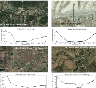
nature of their evolution. Wide bedrock valleys and their evolutionary descendants, strath terraces, are erosional fea-tures in bedrock that are several times wider than the chan-nels that carved them and range in spatial scale from tens to thousands of meters (Fig. 1). Wide bedrock valleys cre-ated by incising rivers provide the opportunity for sediment storage in the valley bottom, influence hydraulic dynamics by allowing peak flows to spread out across the valley, and decrease the average transport velocity of sediment grains (Pizzuto et al., 2017).
lateral erosion in bedrock rivers. The frequency of intense rain is correlated with higher channel sinuosity and lat-eral erosion rates on regional scales (Stark et al., 2010). Sev-eral studies demonstrate that significant latSev-eral erosion in rapidly incising rivers is accomplished by large flood events (Hartshorn et al., 2002; Barbour et al., 2009) resulting from cover on the bed during extreme flood events (Turowski et al., 2008) and exposure of the bedrock walls to sediment and flow (Beer et al., 2017). Sediment cover on the bed that suppresses vertical incision and allows lateral erosion to continue unimpeded is a critical element for the devel-opment of wide bedrock valleys, as determined from mod-eling, field, and experimental studies (Hancock and Ander-son, 2002; Brocard and Van der Beek, 2006; Johnson and Whipple, 2010). Lateral erosion that outpaces vertical in-cision and creates wide bedrock valleys and strath terraces has been linked to weak underlying lithology, such as shale (Montgomery, 2004; Snyder and Kammer, 2008; Schanz and Montgomery, 2016), although strath terraces certainly ex-ist in stronger lithologies, such as quartzite (Pratt-Sitaula et al., 2004). The relationships among river sediment flux, discharge, lithology, and rates of lateral bedrock erosion are not well defined. Because we do not sufficiently understand the processes of lateral erosion, landscape evolution models lack a physical mechanism for allowing channels to migrate laterally and widen bedrock valleys, in addition to incising bedrock valleys.
Existing landscape evolution models do not address the lateral erosion of bedrock channel walls and the consequen-tial migration of the channel, in no small part because of the lack of a rigorous understanding of the processes that control the lateral erosion of bedrock channel walls. If this theoretical hurdle can be cleared, an algorithm for lateral erosion must be applied within a framework of models that currently only erode and deposit vertically. To our knowl-edge, this study is the first attempt at incorporating a gen-eralized physics-based algorithm for lateral bedrock erosion and channel migration on a drainage basin scale to a two-dimensional landscape evolution model.
2 Background
Theories for the vertical incision of bedrock channels have advanced considerably since the first physics-based bedrock incision models were presented in the early 1990s. For ex-ample, bedrock incision models now include theories for the adjustment of channel width (e.g., Stark and Stark, 2001; Wobus et al., 2006; Turowski et al., 2009; Yanites and Tucker, 2010), the role of sediment size and bed cover (e.g., Whipple and Tucker, 2002; Sklar and Dietrich, 2004; Yanites et al., 2011), and thresholds for incision (e.g., Tucker and Bras, 2000; Snyder et al., 2003b). Rivers may re-spond to changing boundary conditions by adjusting both slope and channel width (Lavé and Avouac, 2001; Duvall
et al., 2004; Snyder and Kammer, 2008, e.g.,) and landscape evolution models must be able to capture both of these re-sponses if we are to fully describe the behavior and function of landscapes. Research on bedrock channel width gives im-portant insights into the larger-scale problem of bedrock val-ley widening. In particular, sediment cover on the bed plays an important role in the evolution of channel cross-sectional shape because sediment cover on the bed can slow or halt vertical incision (Sklar and Dietrich, 2004; Turowski et al., 2007) while allowing lateral erosion to continue. Models of channel cross-sectional evolution predict that increasing sediment supply to a steady-state stream results in a wider, steeper channel for a given rate of base-level fall (Yanites and Tucker, 2010). While theories that account for dynamic adjustment to bedrock channel width continue to be refined (for a review, see Lague, 2014), landscape evolution models that include a relationship between sediment size and cover (Gasparini et al., 2004) and incision thresholds in bedrock channels (Tucker et al., 2001; Crave and Davy, 2001; Tucker et al., 2013) are available and widely used (Tucker and Han-cock, 2010).
Numerical models for alluvial rivers have made consid-erable advances in capturing the planform dynamics of both meandering and braided rivers, which necessarily include lat-eral bank erosion. Howard and Knutson (1984) developed the first numerical model that simulates lateral bank movement in alluvial rivers and produces realistic patterns of river me-andering. In this study, bank erosion scales inversely with the radius of curvature such that more rapid erosion occurs in tighter bends with a smaller radius of curvature. A more recent treatment of radius of curvature as a control on lateral erosion rates has been implemented in CAESAR, a cellular landscape evolution model that calculates a two-dimensional flow field (Coulthard et al., 2002, 2013; Coulthard and van de Wiel, 2006). This model is appropriate for studying alluvial river dynamics in meandering or braided streams at reach and small catchment scales and timescales of up to thousands of years (Van De Wiel et al., 2007), but it is not designed to model the evolution of bedrock rivers. The EROS model is a morphodynamic–hydrodynamic model that also allows for the lateral erosion of bank material (Crave and Davy, 2001; Davy and Lague, 2009; Carretier et al., 2016). In EROS, the lateral erosion of bank material is equal to the vertical ero-sion rate multiplied by the lateral topographic slope and a coefficient of unknown value (Davy and Lague, 2009). This treatment of lateral erosion allows for lateral channel mobil-ity and the development of realistic braided rivers, but it lacks a mechanistic process specifically for the lateral erosion of bedrock channels.
dis-charge, valley gradient, and sediment grain size (e.g., Hooke, 1975; Schumm, 1967; Nanson and Hickin, 1986; Sun et al., 2001; Lancaster and Bras, 2002; Parker et al., 2011). This body of work addresses the planform pattern of river chan-nels, but does not deal with the broader drainage basin topog-raphy in which those channels are embedded. The principal state variable in channel meander models is the trace of the channel, x(λ), whereλ represents streamwise distance and
x=(x, y, t) is the channel centerline position. Some more
recent models also incorporate a vertical channel coordinate, so that x=(x, y, z, t) (e.g., Limaye and Lamb, 2013), but the emphasis remains on the channel trace rather than on the topography. For example, the slope of the channel and/or val-ley is normally treated as a boundary condition rather as an element of topography that evolves dynamically as it steers the flow of water, sediment, and energy.
There is also a well-developed literature on process mod-els of landscape evolution, in particular the evolution of ridge–valley topography sculpted around drainage networks. We refer to these models as landscape evolution models, or LEMs (e.g., Coulthard, 2001; Willgoose, 2005; Tucker and Hancock, 2010; Valters, 2016; Temme et al., 2017). With LEMs, the emphasis lies on computing the topographic el-evation field, η(x, y, t). Water and sediment cascade pas-sively downhill across this surface. In some of these mod-els, channel segments are assumed to exist as sub-grid-scale features that are free to switch direction arbitrarily as the to-pography around them changes. Other LEMs represent water movement as a two-dimensional flow field, whether through multiple-direction routing algorithms (e.g., Coulthard et al., 2002; Pelletier, 2004; Perron et al., 2008) or with a simpli-fied form of the shallow-water equations (Adams et al., 2017; Simpson and Castelltort, 2006). Regardless of the approach to flow routing, LEMs differ from meander models in treating a self-forming, two-dimensional flow network rather than a single channel reach and in explicitly modeling the evolution of topography.
The lateral migration of bedrock channel walls has only been implemented into landscape evolution models in a limited number of studies (Lancaster, 1998; Hancock and Anderson, 2002; Clevis et al., 2006a; Finnegan and Diet-rich, 2011; Limaye and Lamb, 2013). Hancock and An-derson (2002) model bedrock valley widening using a one-dimensional stream power model for vertical incision and assume that valley widening rates depend on stream power. They note that the width of the valley floor is related to the duration of steady state in the river, as theorized by Suzuki (1982). This model is based on the key observation that lat-eral erosion exceeds vertical incision when the channel is carrying the maximum sediment load dictated by the trans-port capacity. By varying sediment supply to the channel, their model predicts the development of a series of strath terraces. Strath terrace sequences have also been produced by coupling a meandering model with a river incision model (Finnegan and Dietrich, 2011). Clevis et al. (2006a)
mod-eled meandering channels in a valley section using a two-dimensional landscape evolution model and an adaptive grid approach. A vector-based approach to modeling the lateral migration of meandering streams in heterogeneous bed ma-terial has been used to reproduce a range of bedrock valley forms (Limaye and Lamb, 2014), but this model is primar-ily a channel-scale model. While each of these studies model the lateral migration of bedrock channel banks, they all oper-ate with a meandering model that is not applicable to loper-ateral migration in low-sinuosity channels or in a generalized land-scape evolution model.
3 Approach and scope
Until now, landscape evolution models have lacked a generic mechanism for allowing channels to migrate laterally and widen bedrock valleys, as well as incise bedrock valleys. While advances in controls on bedrock valley width have been made using meandering models, the representation of a sinuous channel does not describe all rivers, and often such models are constructed on a channel scale rather than on a drainage basin scale. In this study, we develop a theory for the lateral migration of bedrock channel walls and imple-ment this theory in a two-dimensional landscape evolution model for the first time. We seek to explore the parameters that exert primary control on the morphology of bedrock val-leys and the rate of bedrock valley widening using a series of numerical experiments.
With a few exceptions noted below, most LEMs treat ero-sion and sedimentation as purely vertical processes. When the flow of water and sediment collects in a “digital valley”, the elevation of that location may rise or fall, but lateral ero-sion by channel impingement against a valley wall is usu-ally neglected. Yet nature seems to be perfectly capable of forming erosional river valleys much wider than the chan-nels they contain (Fig. 1). The question arises of how one might honor the process of valley widening by lateral ero-sion (and narrowing by inciero-sion) within the topographically oriented framework of an LEM. In other words, how might the key features of LEMs and channel planform models be usefully combined?
In addressing this issue, it is useful to consider that the typical LEM treatment of topography as a two-dimensional fieldη(x, y, t) is itself a simplification, albeit a practical one. Consider an alternative framework in which the boundary between solid material (rock, sediment, soil) and fluid (air, water) is treated as a surface in three-dimensional space,
σ(x, y, z, t) (Braun et al., 2008). The surface possesses at
complexity. For practical reasons, it is desirable to find meth-ods by which a lateral component of erosion by stream chan-nels could be represented within the much simpler frame-work of a two-dimensional elevation fieldη(x, y, t).
In this paper, our objective is to define and explore a the-ory for lateral erosion that has the following characteristics: simple and sufficiently general in nature to be applicable in landscape evolution models; containing as few parame-ters as possible; requiring relatively few input variables, such as channel gradient and water discharge plus gross channel planform configuration. The aim of this theory is to model valley widening or narrowing over timescales relevant to drainage basin evolution and across multiple branches within a drainage network. The theory is not designed to predict the movement of a particular channel segment over a period of a few years, but rather is intended to provide a general basis for understanding when and why valleys tend to narrow or widen during the course of their long-term geomorphic evo-lution. Theoretical predictions about these trends then serve as quantitative, mechanistically based hypotheses that can be tested through experiments and observations. Through a set of numerical experiments, we seek to answer the following set of questions.
– How does this lateral erosion model compare with purely vertical erosion models?
– How do two alternative formulations, which treat bank material differently, compare to each other?
– What combinations of bedrock erodibility, sediment mobility, water flux, sediment flux, and model type re-sult in wide bedrock valleys?
– What are the predictions of the model that could be readily tested through experiment and/or observation?
In the following sections we outline our theory for lateral channel wall migration and explain the two algorithms we have developed to apply this theory to an existing model. We then present the results from our set of numerical exper-iments and discuss how well the model describes the forma-tion of wide bedrock valleys. The approach presented here is intended to be a starting point, but not an ending point. Our main goal is to draw attention to the importance of lateral stream erosion within the context of drainage basin evolu-tion and to offer some ideas for how this might be addressed in the framework of a conventional grid-based LEM.
4 Theory
We have deliberately chosen the most simple formulation possible for deposition and erosion, while still capturing the role of sediment. We do this in order to focus on developing the lateral erosion component of our model. Evolution of the height of the landscape,η, through time is described by the
deposition rate,d, minus the erosion rate,e, plus a constant rate of uplift relative to base level,U.
∂η
∂t = −e+d+U (1)
The deposition rate is assumed to depend on the concentra-tion of sediment (Cs) in active transport and its effective
set-tling velocity,νs. Sediment concentration is expressed as the
ratio of volumetric sediment flux,Qs, to water discharge,Q:
Cs=
Qs
Q. (2)
We treat water discharge as the product of runoff rate and drainage area such thatQ=RA. The deposition rate is there-fore given by
d=νsd∗Qs
RA , (3)
whered∗ is a dimensionless number describing the vertical
distribution of sediment in the water column, which is equal to 1 if sediment is equally distributed through the flow (Davy and Lague, 2009); νs, d∗, and R are lumped into a single
dimensionless parameter,α, that represents the potential for deposition.
α=νsd∗
R (4)
A large value forαimplies more rapid deposition (all else being equal) either because settling velocity,νs, is high and
sediment is quickly lost from the flow, or because runoff rate,
R, is low and there is little water in the channels to dilute the sediment. A small value forαrepresents slower settling velocity, or more intuitively, greater runoff;αcan be thought of as a sediment mobility number. Whenα <1, sediment is easily transported and the model tends towards detachment-limited behavior. Whenα >1, sediment is less mobile and the model tends towards transport-limited behavior.
4.1 Vertical erosion theory
In the model presented here, we use the stream power inci-sion model (e.g., Howard, 1994) to calculate the vertical in-cision rate; the stream power model is the simplest bedrock incision model that represents fluvial erosion for steady-state topography. The vertical erosion rate is derived from the rate of energy dissipation on the channel bed, which is given by
ωv=ρg
Q
WS, (5)
whereρ is the density of water, g is gravitational acceler-ation,Qis water discharge, W is channel width, and S is channel slope. We assume that the rate of vertical erosion scales as
Ev=Kv0
ωv
Ce
Figure 1.Field examples of wide bedrock valleys cut by lateral erosion. All cross sections are from north to south.(a)The Drôme River in the French Alps is transport limited and meandering in reaches that carve wide bedrock valleys. The bedrock valley at this location (44.69◦N, 5.14◦E) is 500 m wide and the channel is∼45 m wide (indicated by light blue shade of cross section line).(b)Gower Gulch (36.41◦N, 116.83◦W) in Death Valley, USA widened significantly in response to increased discharge from a stream diversion in the 1940s (Snyder and Kammer, 2008). The bedrock valley is 30 m wide and the channel braids are∼2 m wide (indicated by light blue shade of cross section line).(c)Left Hand Creek drains the Colorado Front Range (40.11◦N, 105.25◦W) and has undergone multiple cycles of lateral erosion that produced flights of strath terraces, outlined in white on the image. The cross section shows Table Mountain at∼70 m above the current stream height on the north side of cross section and a lower terrace level at 10 m above the current stream level on the south side of the cross section.(d)Arroyo Seco in the California Coast Range (36.27◦N, 121.33◦W) carved a 600 m wide strath terrace during a period of lateral erosion that is 30 m above the current stream level. The current bedrock valley is 125 m wide and the channel is∼15 m wide (indicated by light blue shade of cross section line). Images: Google Earth. Cross sections: NCALM and 30 m SRTM.
whereKv0 is a dimensionless vertical erosion coefficient and
Ce is cohesion of bed and bank material. We use bulk
co-hesion simply as a convenient reference scale for rock resis-tance to erosion. This choice allows us to express the ero-sion rate as a function of the hydraulic power applied (ωv),
a commonly used measure of material strength (Ce), and a
dimensionless efficiency factor (Kv0).
We assume that channel width is a function of discharge (Leopold and Maddock, 1953):
W =kwQ0.5, (7)
where kw is a width coefficient. It is important to
recog-nize that channel width is not explicitly represented in the model we describe. Rather, it is one element of the lumped parameters Kv and Kl (erosion coefficients discussed
be-low). The channel-width scaling parameter values we dis-cuss (kw) are used only in the estimation of reasonable ranges
for these parameters. The bank width coefficient,kw, is
be-tween channel width and discharge. SubstitutingRAforQ
and Eq. (7) forWin Eq. (5) and then combining Eqs. (5) and (6) gives the following:
Ev =
Kv0ρgR1/2 kwCe
A1/2S, (8a)
Ev =KvA1/2S. (8b)
Lumping several parameters givesKv, a dimensional
verti-cal erosion coefficient (with units of years−1) that consists of known or measurable quantities, and one unknown dimen-sionless parameter,Kv0.
Although evidence indicates that sediment in the channel plays an important role in inciting lateral erosion in bedrock channels (Finnegan et al., 2007; Johnson and Whipple, 2010; Fuller et al., 2016), the model presented here uses the stream power incision model to represent vertical erosion, which does not account for sediment-flux-dependent incision (e.g., Beaumont et al., 1992; Sklar and Dietrich, 2004; Turowski et al., 2007). The standard stream power model (Eq. 8) has some limitations, especially in the lack of threshold effects and the assumption of constant channel width (Lague, 2014). Despite these limitations, the stream power model is a good approximation for long-term vertical bedrock incision on large spatial scales (e.g., Howard, 1994; Whipple and Tucker, 1999) and is appropriate here given that the goal of this work is to explore the dynamics of lateral bedrock erosion as a function of channel curvature.
4.2 Lateral erosion theory
Lateral erosion requires hydraulic energy expenditure to damage the bank material and/or dislodge previously weath-ered particles (Suzuki, 1982; Lancaster, 1998; Hancock and Anderson, 2002). Consistent with earlier meandering mod-els (e.g., Howard and Knutson, 1984), we hypothesize that the lateral erosion rate is proportional to the rate of energy dissipation per unit area of the channel wall created by cen-tripetal acceleration around a bend. Erosion of the channel wall is the result of the force of water acting on the chan-nel wall. We know from basic physics that the force of water acting on the wall is equal to the force of the wall acting on the water, which is equal to centripetal force. Centripetal force isFc=mv
2
rc, wheremis mass,vis velocity, andrcis
the radius of curvature. The centripetal force of a unit of wa-ter can be found by replacing m withρLH W, whereρ is the density of water andL,H, andW are unit length, water depth, and channel width, respectively. The centripetal force of water flowing around a bend can be expressed in terms of centripetal shear stress, which is analogous to bed shear stress, by dividing both sides byH L, giving
σc=
ρW v2
rc
. (9)
Centripetal shear stress can be turned into a rate of energy expenditure by multiplying by fluid velocity, giving
ωc=
ρW v3
rc
. (10)
To express this in terms of discharge,Q, instead of veloc-ity, we employ the Darcy–Weisbach equation, givingv3=
gqS/F, whereqis discharge per unit width andF is a
fric-tion factor, which yields
ωc=
ρgQS rcF
. (11)
Equation (11) describes a quantity that might be termed cen-tripetal unit stream power, as it represents the rate of energy dissipation per unit bank area. The centripetal unit stream power is similar to the more familiar quantity unit stream power, except that channel width is replaced by the radius of curvature multiplied by a friction factor.
We hypothesize that lateral erosion rate scales with energy dissipation rate around a bend according to
El=Kl0
ωc
Ce
, (12)
whereKl0is a dimensionless lateral erosion coefficient. Com-bining Eqs. (11) and (12) gives
El =
Kl0ρgR CeF
AS rc
, (13a)
El =Kl
AS rc
, (13b)
whereKlis a dimensional erosion coefficient for lateral
ero-sion composed of known or measurable quantities and one unknown dimensionless parameter,Kl0. IfKl0is equal toKv0, we find a ratio betweenKlandKvgiven by
Kl
Kv =R
1/2k w
F , (14)
which consists of runoff rate,R, bank width coefficient,kw,
and friction factor,F. We can measure or make reasonable estimates of each of these parameters in order to determine what the ratio of lateral to vertical erodibility should be. Mean annual runoff rate can vary widely, but a higher peak runoff intensity will lead to a higherKl/Kvratio and more
lateral erosion.
A fixed kw is common in landscape evolution
mod-els that model long-term landscape erosion (e.g., Tucker et al., 2001; Gasparini et al., 2007), but channel width can vary with incision rate in models and natural sys-tems (Yanites and Tucker, 2010; Duvall et al., 2004), sug-gesting there are cases when dynamic width scaling is im-portant (Lague, 2014). In this model, kw is given a value
(Leopold and Maddock, 1953), but the value can range be-tween 1 and 10 due to differences in runoff variability, sub-strate properties, and sediment load (Whipple et al., 2013). The friction factor, F, is the Darcy–Weisbach friction fac-tor, which can range from 0.01–1.0 for natural rivers (Gilley et al., 1992; Hin et al., 2008). With a lower friction factor (representing smooth channel walls), the lateral erosion ra-tio would be higher due to less energy being dissipated on the channel walls, leaving more energy available for lateral erosion.
5 Numerical implementation
One challenge in modeling both vertical and lateral erosion in a drainage network lies in the representation of topogra-phy. Typically, landscape evolution models use a numerical scheme in which the terrain is represented by a grid of points whose horizontal positions are fixed and whose elevation rep-resents the primary state variable in the model. Such a frame-work does not lend itself to the motion of near-vertical to vertical interfaces (such as stream banks and cliffs), and for this reason, incorporating lateral stream erosion in a conven-tional landscape evolution model requires a modification to the basic numerical framework. A vertical rather than hor-izontal grid (Kirkby, 1999) can be used for near-vertical landforms in isolation, but is inappropriate when one wishes to represent vertical interfaces that are inset within a larger landscape. Grid-node movement combined with adaptive re-gridding (Clevis et al., 2006a, b) provides a possible solu-tion, but is computationally expensive and particularly dif-ficult to implement when multiple branches of a drainage network may undergo lateral motion. Here, we adopt a sim-pler approach in which valley walls are viewed as sub-grid-scale features that migrate through the fixed grid. Rather than tracking the position of these vertical interfaces, we instead track the cumulative sediment volume that has been removed from the cell surrounding a given grid node as a result of lat-eral erosion. When that cumulative loss exceeds a threshold volume, the elevation of the grid node is lowered.
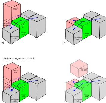
More specifically, at each node in the model, we calcu-late a vertical incision rate at the primary node and a lat-eral erosion rate at a neighboring node (Fig. 2). The latlat-eral neighbor node for the primary node is chosen on the out-side bank of two stream segments that flow into and out of the primary node. The stream segments used to identify the neighboring node over which lateral erosion should occur are the incoming stream segment to the primary node with the greatest drainage area and the stream segment that connects the primary node to its downstream neighbor (Fig. 2). If the two segments are straight, then a neighboring node of the pri-mary node is chosen at random and lateral erosion occurs at this node until elevation changes at the node.
The calculation of the radius of curvature along two stream segments in a raster grid with D8 flow routing presents a
challenge, as the angle between segments is discretized; the two segments may form a straight line, in which case the an-gle is equal to 0◦, form a 45◦angle, or form a 90◦angle. In
order to reduce the impact of this discretization, we assume that each of these three cases represents a continuum of pos-sible radii of curvature. Cases of two straight segments are treated as if the actual angle between them ranges anywhere between+22.5 and−22.5◦. If one takes the average among these possible angles, the resulting inverse radius of curva-ture is 0.23/dx, where dxis the cell size in the flow direction. Similarly, we assume that a 45◦ bend represents a contin-uum of possible angles between the two segments ranging from 22.5–63.5◦, resulting in an inverse radius of curvature of 0.67/dx. Following the same principle for a 90◦bend gives a mean inverse radius of curvature of 1.37/dx (see the Sup-plement).
The volumetric rate of material eroded laterally for each lateral node is calculated byEl×dx×H, whereHis water
depth given in meters. Water depth at each node is calcu-lated byH=0.4Q0.35 (Andrews, 1984), where Qis given in m3s−1. The volume of sediment eroded laterally per time step is sent downstream along with any material eroded from the primary cell. The volumetric erosion rate is multiplied by the time step duration to get the volume eroded at the lateral nodes, and the cumulative volume eroded from each lateral node is tracked throughout the entire model run. When the cumulative volume eroded from the lateral node equals or ex-ceeds the volume needed to erode the node (see end-member model descriptions below), the elevation of the lateral node is set to the elevation of the downstream node (Fig. 2). Flow is then rerouted and water flows down the path of steepest de-scent. The model does not distinguish between sediment and bedrock in the model grid and all material that is eroded has the bedrock erodibility of theKvorKlterms. When material
is eroded vertically or laterally from bedrock nodes, the vol-ume of the eroded material is sent downstream as part of the
Qs term. If deposition occurs in the model, deposited
mate-rial is added to the topography of the node as bedrock. Thus, sediment is not “seen” in the model as material that can be easily re-eroded after deposition; rather, sediment works to increase the deposition term (Eq. 3).
H
El
Ev Sediment
downstream
Primary node Lateral
node
Downstream node
Primary node Downstream
node
H
El
Ev Sediment
downstream
Primary node Lateral
node
Downstream node
Primary node Downstream
node "Slumped"
material
(a) (b)
(c) (d)
Total block erosion model
Undercutting-slump model
Figure 2.Conceptual illustration of model nodes showing the stream segments (in light blue) from the upstream node, to the primary node (in green), to the downstream node. Vertical erosion (Ev) occurs at the primary node. The neighbor node (in pink) where lateral erosion
(El) occurs is located on the outside bend of the stream segments. The height over which lateral erosion occurs,H, is shown by the dashed
blue line.(a)For the total block erosion model, the volume that must be laterally eroded before elevation is changed is (Zn−Zd)dx2, the
difference in elevation between the neighbor node and the downstream node (indicated with double-sided black arrow) times the surface area of the neighbor node.(b)The elevation of the lateral node is changed after the entire block is eroded and flow can potentially be rerouted.
(c)In the undercutting-slump model, the volume that must be laterally eroded (representing bank undercutting) before elevation is changed is (H−Zd)dx2.H−Zdis the difference in elevation between the water surface height and the elevation of the downstream node, indicated
with the double-sided black arrow.(d)When the neighbor node has been undercut, elevation is changed, allowing water to be rerouted, while the slumped material is transported downstream as wash load.
End-member model formulations
We have implemented two methods of determining whether enough lateral erosion has occurred to lower the lateral node. The first method, the total block erosion model, dictates that the entire volume of the lateral node above the elevation of the downstream node must be eroded before its eleva-tion is changed (Fig. 2a, b). This formulaeleva-tion assumes that the height of the valley walls is a controlling factor in the ultimate width a valley can achieve, and thus valley width scales with valley wall height. In this method, lateral migra-tion depends on bank height so that taller banks experience
slower lateral migration, as all of the volume of the lateral node must be eroded for the valley to widen. The second method, the undercutting-slump model, dictates that only the volume of the water height on the bank times the cell area must be eroded for the elevation to change (Fig. 2c, d), while the remaining material slumps into the channel and is trans-ported away as wash load, i.e., not redeposited in the model or included inQscalculations. This model formulation
lat-eral channel migration and valley width in transport-limited streams where additional sediment from valley walls can-not be transported out of the channel (Nicholas and Quine, 2007; Bufe et al., 2016; Malatesta et al., 2017). However, whether valley wall height should limit valley widening in detachment-limited bedrock channels is less clear (Lan-caster, 1998) and likely depends on the bedrock lithology (Finnegan and Dietrich, 2011; Johnson and Finnegan, 2015). The links between these end-member model formulations and the natural processes they represent are explored in the Discussion section.
6 Model experiments
In order to constrain the conditions that result in significant lateral bedrock erosion and valley widening, we ran sets of models using a range of values for bedrock erodibility, α
(sediment mobility number), and theKl/Kvratio using both
the total block erosion model and the undercutting-slump model (Table 1). The model domain was 600 m by 600 m with a 10 m cell size, three closed boundary edges, and an uplift rate relative to base level of 0.0005 m yr−1 imposed on the entire model domain. Water flux was introduced at the top of the model by designating a node as an inlet with an area of 20 000 m2 and sediment flux at carrying capac-ity. This setup allowed each run to have a primary channel on which to measure width and channel mobility. All mod-els were spun up to an initial condition of approximately uniform erosion rate with vertical incision only. The mod-els were then run for 100–200 kyr with the lateral erosion component. In order to isolate the effect of bedrock bility, a set of model calculations was run in which erodi-bility ranged from 5×10⁻⁵to 2.5×10⁻⁴(Stock and Mont-gomery, 1999) whileαwas held constant at 0.8. In order to isolate the effect of detachment-limited vs. transport-limited behavior, another set of models was run in which erodibil-ity was held constant at 1×10⁻⁴andαvalues ranged from 0.1 to 2, which represents a detachment-limited system when
α <1 and a transport-limited system whenα >1 (Davy and
Lague, 2009) (Table 1).Kl/Kvratios for all model runs were
set to 1.0 or 1.5, resulting in a runoff rate of 14 or 36 mm h−1 from Eq. (14). These runoff rates do not represent a yearly mean annual runoff, but rather peak event runoff rates that are likely to result in appreciable lateral erosion due to the scaling with theKl/Kvratio. Small et al. (2015) found that
bedrock erosion rates in abrasion mill experiments are an or-der of magnitude higher in samples from channel margins compared to the channel thalweg. This suggests that Kl in
this model should be at least equal toKvand could be much
higher (Finnegan and Dietrich, 2011).
Understanding the model behavior in response to detachment- vs. transport-limited behavior (represented by
α) and theKl/Kvratio is complex and requires
understand-ing how runoff plays into both parameters. The value ofαis
calculated byvs, a proxy for grain size, and runoff rate,R,
although neither grain size nor runoff is explicitly set in the model runs. Values ofαthat capture a range of detachment-or transpdetachment-ort-limited behavidetachment-or are set instead (α=0.2–2.0). When the Kl/Kv ratio is set for a given model (either 1.0
or 1.5 in all model runs), the runoff rate is calculated inside the model. Once a runoff rate for a givenKl/Kvratio is
cal-culated, by extension a value ofvs can be calculated from
runoff rate and the setαvalue. Therefore, in model runs with the sameKl/Kvratio and therefore the same runoff rate, a
transport-limited system (αgreater than 1) has a larger grain size (approximated byvs) compared to a detachment-limited
system with a lowα.
6.1 Measures of lateral erosion in model landscapes 6.1.1 Channel mobility
Channel mobility distinguishes models with lateral erosion from models with only vertical incision. At steady state, channels in models with only vertical bedrock incision do not migrate across the model domain. However, a mobile chan-nel is necessary to carve wide valleys and it is enticing to say that the more mobile the channels, the wider the bedrock valley. In our model, channel mobility is not controlled by sediment flux, as found in alluvial channels (Wickert et al., 2013; Bufe et al., 2016), but by the lateral erosion of bedrock. However, the term “channel mobility” is used here in the same sense as in the alluvial literature; channel mobility de-scribes lateral channel planform changes along the length of the channel.
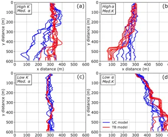
The effect of bedrock erodibility andαon channel migra-tion through time for both model versions is shown in Fig. 3. Channel migration over 200 kyr is shown for six selected runs that span the range of bedrock erodibility andαvalues for the two different model formulations: the undercutting-slump model in whichKl/Kv=1.5 and the total block
ero-sion model in whichKl/Kv=1.5. In all runs, the total block
erosion model produced more confined channels compared to the undercutting-slump model. The undercutting-slump model produces more dynamic channel migration over the model domain, especially in the highKmodel. In both model formulations, the highKand highαruns have the widest ex-tent of channel migration (recall that highαrepresents lower sediment mobility) and the lowK and lowαruns have the most restricted channel migration.
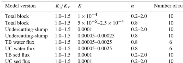
Table 1.Model runs and parameters discussed in this paper.
Model version Kl/Kv K α Number of runs
Total block 1.0–1.5 1×10⁻⁴ 0.2–2.0 10
Total block 1.0–1.5 5×10⁻⁵–2.5×10⁻⁴ 0.8 10 Undercutting-slump 1.0–1.5 0.0001 0.2–2.0 10 Undercutting-slump 1.0–1.5 0.00005–0.00025 0.8 10 TB water flux 1.0–1.5 0.00005–0.0025 0.8 6 UC water flux 1.0–1.5 0.00005–0.0025 0.8 6
TB sed flux 1.0–1.5 0.0001 0.2–2.0 10
UC sed flux 1.0–1.5 0.0001 0.2–2.0 10
cumulative migration metric, λ, which indicates how often the channel has migrated during the model run. A model run can have the sameλvalue if the channel marches across the entire model domain or if the channel repeatedly switches between two nearby channel courses;λcan also be used as an indicator for the maximum lateral extent occupied by the channel during the model run. That is, the maximum possi-ble extent ofxpositions occupied by the channel is equal to
λ, but the actual x distance occupied by the main channel could be lower as the channel migrates over the same area repeatedly.
Bedrock erodibility and theKl/Kvratio have the strongest
control on channel migration distance. Channel mobility increases as bedrock erodibility increases in both the to-tal block erosion model and the undercutting-slump model (Fig. 4a, b). When K is low, representing strong bedrock lithology, there is limited channel movement in the total block erosion models with λ values between 15 and 35 m. This means that on average during the model run the chan-nel occupied 1–3 cells (Fig. 3c). With low values ofK, the undercutting-slump model hadλvalues around 200 m, but a lateral extent of only 5 model cells (Fig. 3c). This indicates that in the undercutting-slump model, the channel was ac-tively migrating within a small area of the model domain. In model runs with highK values representing weak bedrock, total channel migration,λ, and the spatial extent of the chan-nel migration increase (Fig. 3a). With the total block model,
λ appears to be a good proxy for the total spatial extent of channels, but for the undercutting-slump model,λ tends to overestimate the lateral extent of channel occupation (Fig. 3). Increasing theKl/Kvratio from 1.0 to 1.5 results in 1.5–
2 times more channel mobility, with the largest relative in-creases in total block erosion model runs with high erodi-bility and higher αvalues (Fig. 4a, b). This is because the undercutting-slump models already have high channel mo-bility withKl/Kv equal to 1. Increasing theKl/Kvratio to
1.5 increases channel mobility in UC models, but the total block erosion models have a larger threshold for lateral ero-sion, so the increasedKl/Kvratio results in relatively more
channel mobility in the total block models.
For model runs with the same bedrock erodibility but dif-ferentαvalues (which represents sediment mobility), chan-nel mobility is lower in models with lower values ofα (rep-resenting high sediment mobility) and higher when α >1 (representing less mobile sediment; Fig. 4b). In the following presentation and discussion of models with varying values of
α, highαmodel runs will be termed “transport limited” and lowαmodel runs will be termed “detachment limited”. This effect is most pronounced in the total block erosion models in which channel mobility increases by a factor of 4 asα in-creases. In the undercutting-slump models, channel mobility also increases withα, especially whenKl/Kv=1.5. When
Kl/Kv=1 in the undercutting-slump models, the trend in
channel mobility vs.αis less well defined.
6.1.2 Valley width
Valley width is the primary indicator of lateral erosion; a wide bedrock valley implies that significant lateral erosion has occurred relative to vertical incision. Valleys can be de-fined in a few different ways and valley width needs to be quantified in our model. Many studies use low gradient ar-eas of a DEM to determine valley width (e.g., Brocard and Van der Beek, 2006; May et al., 2013). This gives the width for the valley bottom that has been shaped by channel pro-cesses, but excludes areas that have been recently shaped by channel processes and then reworked by hillslope pro-cesses. Another way to measure valley width is by deter-mining the width of the valley at a certain height above the channel. This simple metric is often used for finding valley width in the field, for example using eye height above the channel (e.g., Snyder et al., 2003a; Whittaker et al., 2007). Using a certain height above the channel to determine valley width in the models cannot distinguish between a fluvially carved bedrock valley and low relief in a landscape with weak bedrock. Instead we define valley width as the width of the area perpendicular to the main channel where slope is characteristic of the fluvial channel rather than hillslopes for a given bedrock erodibility andαvalue. The reference slope for a fluvial channel is given by the slope–area relationship, assuming that the height of the landscape andQs are steady
0 100 200 300 400 500 600 x distance (m)
0 100 200 300 400 500 600 y d ista nc e ( m) high K med. high K med. high K med. high K med. high K med. high K med. high K med. high K med. high K med. high K med. high K med. high K med. high K med. High K Med.
0 100 200 300 400 500 600 x distance (m)
0 100 200 300 400 500 600 y d ista nc e ( m) high med.K high med.K high med.K high med.K high med.K high med.K high med.K high med.K high med.K high med.K high med.K high med.K high med.K High Med.K
0 100 200 300 400 500 600 x distance (m)
0 100 200 300 400 500 600 y d ista nc e ( m) low K med. low K med. low K med. low K med. low K med. low K med. low K med. low K med. low K med. low K med. low K med. low K med. low K med. Low K Med.
0 100 200 300 400 500 600 x distance (m)
0 100 200 300 400 500 600 y d ista nc e ( m) low med.K low med.K low med.K low med.K low med.K low med.K low med.K low med.K low med.K low med.K low med.K low med.K low med.K Low Med.K UC model TB model (a) (b) (d) (c)
Figure 3.Channel positions over 200 kyr with different values for bedrock erodibility andαin the undercutting-slump model (UC model, blue lines) and total block erosion model (TB model, red lines).(a)High bedrock erodibility (K=2.5×10⁻⁴), mediumαvalue (α=0.8).
(b)Highαvalue, indicating low sediment transport (α=2.0), medium bedrock erodibility (K=10−4).(c)Low bedrock erodibility (K= 5×10⁻⁵), mediumαvalue (α=0.8).(d)Lowα, indicating high sediment transport (α=0.2), medium bedrock erodibility (K=10−4).
Eqs. (1) and (3) are combined and rewritten as
U=e−νsd∗Qs
RA . (15)
At steady state, Qs is the total upstream eroded material
given byQs=AU. Substituting the steady-state equation for
Qsand Eq. (8) into Eq. (15) gives
U=KvA1/2S−αU. (16)
Solving the above equation forS gives the equation for ref-erence slope that determines whether a model cell is shaped by fluvial or hillslope processes (Davy and Lague, 2009).
S= U
KvA1/2
(α+1) (17)
Our models successfully produce bedrock valleys that are several model cells wider than the channels that created them (Fig. 5). Models with only vertical incision have v-shaped valleys that are only 1 model cell wide (10 m in our experi-ments) and the channels do not shift laterally (Fig. 5a). Given the specifications of the total block and undercutting-slump models, it is not surprising that the total block models take longer to respond to the onset of lateral erosion and valleys are more narrow than in the undercutting-slump models. The
total block erosion models take on the order of 10 kyr to pro-duce an observable response to lateral erosion and ultimately produce bedrock valleys that are up to 25 m wide, while the undercutting-slump models take about 5 kyr to show a re-sponse to lateral erosion and ultimately produce valleys that are up to 50 m wide.
char-Figure 4.Cumulative channel-averaged migration(a, b)and mean valley width(c, d)averaged over 100 kyr for spin-up models with no lateral erosion (spin, black triangles), total block erosion models (TB, red markers), and undercutting-slump models (UC, blue markers) with Kl/Kv=1 (square markers) and 1.5 (circle markers).(a)Cumulative channel-averaged migration (λ) for model runs withα=0.8 plotted
against bedrock erodibility,K;(b)λfor model runs withK=10−4plotted againstα. Mean valley width averaged over 100 kyr of the model runs.(c)Mean valley width for model runs withα=0.8 plotted against bedrock erodibility,K.(d)Mean valley width for model runs with K=10−4plotted againstα.
Figure 5.Model topography and cross sections aty=500 showing examples of valley widening. The black line indicates the position of the main channel on the landscape. The red triangle shows the position of the main channel in the cross section.(a)Model with vertical incision only.(b)Total block erosion model after 70 kyr of lateral erosion.(c)Undercutting-slump model after 50 kyr of lateral erosion.
acteristic fluvial slope as the criterion for a valley in all model runs gives valley width resulting from lateral erosion, and not valley width inherent in the model, we first use this criterion to measure valley width for the spin-up models that include
Total block erosion models Undercutting-slump models
Low α
High α
(a) (b)
(c) (d)
Slope
Slope
Figure 6.Slope maps showing fluvially carved valleys in total block erosion and undercutting-slump models with high and low values of α. The white and blue areas in the maps indicate slopes that are characteristic of fluvial channels, i.e., lower than the reference slope value (Eq. 17).(a)Total block erosion model, lowα(detachment limited).(b)Undercutting-slump model, lowα(detachment limited).(c)Total block erosion model, highα(transport limited).(d)Undercutting-slump model, highα(transport limited).
(Fig. 4c). When theKl/Kvratio is increased from 1 to 1.5,
valley width increase slightly for all model runs, but wide valleys are not possible in the total block erosion model with this value ofα. Valley width in the undercutting-slump model for changing bedrock erodibility shows a somewhat counter-intuitive signal (Fig. 4c); the undercutting-slump model re-sults in wider valleys for lower values of bedrock erodibility. The reasons for this signal are discussed in the section below. When α is varied and K is constant, valley width in-creases with the tendency towards transport-limited condi-tions (α >1) in all undercutting-slump models, but only in total block erosion models when theKl/Kvratio is equal to
1.5 (Fig. 4b). The widest valleys for a given bedrock erodi-bility occur with high αvalues as a result of higher slope. The models predict more channel mobility and wider val-leys under transport-limited streams (set by α) compared to detachment-limited streams (Fig. 4b, d). Asαincreases, the deposition term increases, and a steeper slope is needed to maintain the landscape in steady state relative to uplift. Higher channel slopes in transport-limited model runs also cause increased lateral erosion according to Eq. (14).
6.1.3 Linking channel mobility and valley width
We have shown that the greatest channel mobility occurs in the undercutting-slump models and increases significantly with increasingly soft bedrock (Fig. 4a). However, maxi-mum channel mobility does not translate into maximaxi-mum ley width. In the undercutting-slump models, the widest val-leys occur in the low erodibility model runs that have rel-atively low channel mobility. This reflects the fact that the areas visited by the migrating channel in the low-relief, high
load. However, models that have resistant bedrock (lowK) are least suitable for the undercutting-slump model. In or-der for this model to be a good description of how nature works, the bed material would need to be able to break up into small pieces that are easily transported away, which is conceivable for resistant clay banks. However, the total block erosion model is generally more appropriate for representing the erosion of resistant bedrock channels that erode into ma-terial transported as bedload.
6.2 Adding complexity: water flux, sediment flux 6.2.1 Effects of increased discharge on lateral channel
migration
In order to investigate how transience in landscapes affects lateral erosion, we introduce increased discharge at the inlet point in the upstream end of the model. Using drainage area as a proxy for discharge, increasing water flux in the model represents how a larger stream on the same landscape influ-ences valley width. Increasing drainage area also allows us to observe the extent of landscape change and how rapidly the different model runs respond to an event such as stream cap-ture. The drainage area at this input point is increased from 20 000 to 160 000 m2and sediment load is set to the carry-ing capacity of the new drainage area. For a typical model run, the additional drainage area approximately doubles the magnitude of drainage area at the outlet of the main channel in the model domain; i.e., maximum drainage area in model runs increases from∼1×10⁵to∼3×5 m2. Models with in-creased water flux were run using both model formulations,
Kl/Kv=1.0 and 1.5, and erodibility values that ranged from
5×10⁻⁵to 2.5×10⁻⁴with alpha held constant at 0.8 (Ta-ble 1).
Recalling that lateral erosion scales with drainage area (Eq. 14), while vertical incision scales with the square root of drainage area (Eq. 8), we therefore expect that increasing drainage area will increase lateral erosion and valley width in every case for the undercutting-slumping model in which the numerically imposed condition for lateral erosion to oc-cur is much smaller than in the total block erosion model. In the total block erosion model, lateral erosion temporarily stalls because of the volume threshold that must be exceeded before lateral erosion occurs. There is no threshold for ver-tical incision, which speeds up when additional water flux is added to the model.
6.2.2 Total block erosion models
In all of the model runs, increased water flux resulted in in-creased lateral erosion and wider valleys. Figure 7 shows val-ley width averaged over the model domain vs. model time for all of the water flux models. The total block erosion model and undercutting-slump model respond differently to a step change in water flux. The total block erosion models first in-cise vertically to a new steady-state stream profile then erode
laterally as a result of the increased water flux (Fig. 8), while the undercutting-slump model incises vertically and erodes laterally simultaneously (Fig. 9).
Total block erosion models in which the Kl/Kv ratio is
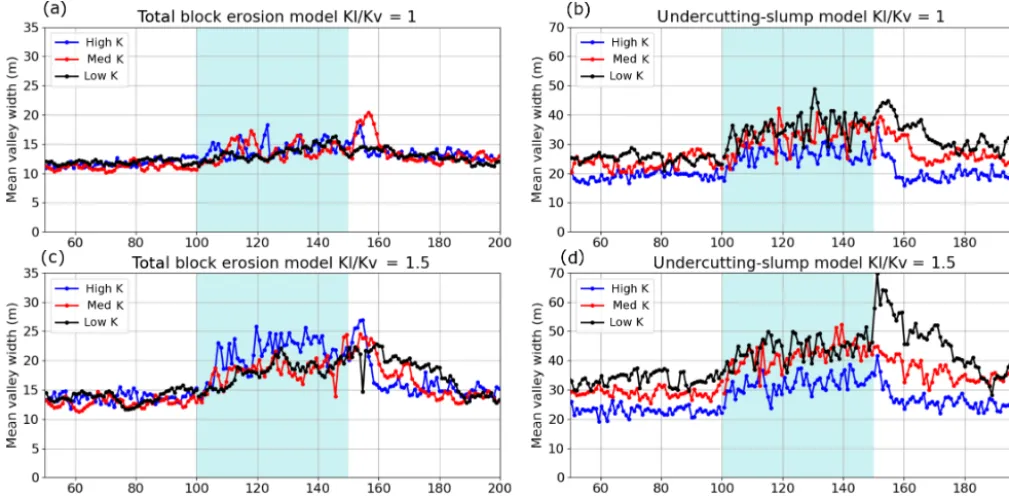
equal to 1.5 (TB1.5) show an interesting pattern in valley widening after increased water flux (Fig. 7c). All of the TB1.5 model runs show a significant increase in valley width during the 50 kyr period of increased water flux. After 6 kyr of increased water flux (model time=106 kyr), the high and medium erodibility model runs have greater valley widths, but the low erodibility model shows a gradual increase in valley width over 14 kyr of increased water flux (model time 100–114 kyr). For the first 14 kyr of the increased water flux, the channel of the low K model run incises rapidly, in-creasing the gradient between the channel and the adjacent cells and preventing lateral erosion. After the channel profile comes into new equilibrium, the increased water flux accel-erates lateral erosion on the valley walls and valleys widen by 10 m compared to before the increased water flux in the total block erosion models.
After the increased water flux stops at 150 kyr, the wider valleys persist for∼10–20 kyr in the low and medium erodi-bility models (Fig. 7c) for two reasons. First, after the ces-sation of increased water flux, the channel returns to equi-librium through aggradation and uplift. While aggradation occurs, lateral erosion can occur more easily in the total block erosion models. In this case, the total volume that must be eroded from any lateral node cell is reduced as the channel floor moves up in vertical space. The second rea-son for persistent wide valleys is that in the medium and lowK model runs, the increase in water flux eroded wide valleys into relatively resistant bedrock. These flat surfaces near the channel persist in harder bedrock, even after water flux has decreased to original levels. Following the end of the period of increased water flux, valley width in the TB1.5 medium K model run remains elevated for 10 kyr (model time 160 kyr) before channel narrowing that propagates up-stream (Fig. 10). After cessation of the increased water flux at 150 kyr, the channel profile returns to equilibrium through uplift and aggradation (Fig. 10a). Channel aggradation be-gins at the bottom of the channel profile and results in a con-vexity that propagates upstream (Fig. 10a). At model posi-tiony=400, from 150–158 kyr the channel increases in el-evation due to uplift (Fig. 10b). Wide valleys created during increased water flux are maintained, and new lateral erosion of valley walls is seen (Fig. 10b). At 159 kyr, 9 kyr after the cessation of increased water flux, the aggradational knick-point reachesy=400 and incision and valley narrowing is observed (Fig. 10d, e).
Figure 7. Valley width averaged over the model domain vs. model time for total block erosion and undercutting-slump models with Kl/Kv=1 and 1.5. Increased water flux occurs from 100 to 150 kyr, indicated by light blue shading.
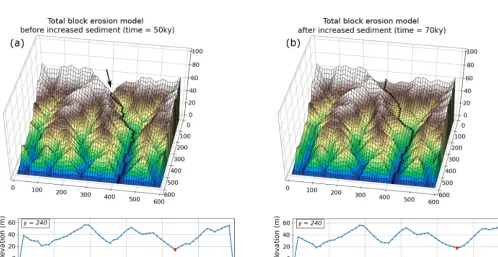
Figure 8.Surface topography and cross section aty=420 during the period of increased water flux for the total block erosion models. The red triangle on cross sections indicates the channel position.(a)Total block erosion model with lowKandKl/Kv=1.0 at 100 kyr before
the increase in water flux. Note that this model looks similar to the spin-up model runs with no lateral erosion.(b)After 15 kyr of increased water flux, the cross section shows vertical incision in the channel and increased relief between the channel and the hillslopes.(c)At 30 kyr after water flux increased, equilibrium is reached. Lateral erosion can begin and the valley widens to 20 m aty=420.
(Fig. 8a). After 15 kyr of increased water flux and increased vertical incision, the topography reaches a new equilibrium and channel elevation is stationary. Only after this period of re-equilibration can lateral erosion begin to widen the val-leys. After 30 kyr of increased water flux, the entire channel has incised, especially in the upper valley. At y=420, the position of the cross section, the channel has been incised by 3 m, and the valley has widened to about 20 m (Fig. 8c). This response of primarily vertical incision is expected when
us-ing the total block erosion model, which sets a high threshold for lateral erosion.
6.2.3 Undercutting-slump models
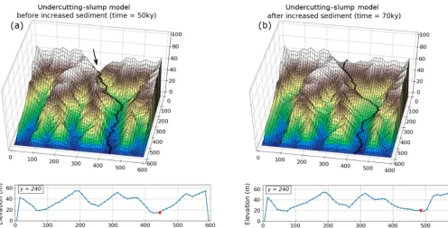
Figure 9.Surface topography and cross section aty=420 during the period of increased water flux for the undercutting-slump models. The red triangle on cross sections indicates the channel position.(a)Undercutting-slump model with lowKandKl/Kv=1.5 at 100 kyr before
the increase in water flux. Valley is 30 m wide.(b)After 15 kyr of increased water flux, the channel has both vertically incised and laterally widened the valley to a width of 40 m.(c)After 30 kyr of increased water flux, the valley has a width of 60 m aty=420.
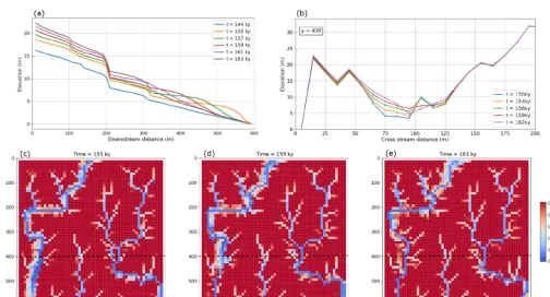
Figure 10.Longitudinal profile, cross sections, and slope maps from model run TB1.5, with mediumKafter cessation of increased water flux.(a)Longitudinal channel profiles show uplift and aggradation, which produces a convexity that propagates upstream.(b)Cross sections across the model domain aty=400 show channel aggradation and new lateral erosion of valley walls.(c, d, e)Slope maps show valley narrowing following the passage of the knickpoint wherey=400 (dashed line) at 155, 159, and 163 kyr.
above. Unlike the total block erosion models, there is no discernible lag between the onset of water flux and valley widening in the undercutting-slump models (Fig. 9). This is because erosion of the valley wall is independent of the height of the valley wall for the undercutting-slump model formulation and the increase in drainage area results in larger increases in lateral erosion rates faster compared to vertical
(Fig. 9a). Following the increase in water flux, the valley is much wider across the entire model domain, especially at the upstream segments of the channel. After 15 kyr of in-creased water flux, the channel has both vertically incised and widened the valley to∼40 m aty=420 (Fig. 9b). After 30 kyr of increased water flux, the valley has widened fur-ther to∼60 m aty=420 (Fig. 9c). The undercutting-slump model runs with medium and low erodibility maintain in-creased valley width after water flux has dein-creased, partic-ularly inKl/Kv=1.5 models (UC1.5) (Fig. 7d). This
indi-cates that wide valley floors can persist for long periods of time after the conditions that created them have stopped.
6.2.4 Effects of increased sediment flux on lateral erosion
In order to explore how the addition of sediment to a stream affects lateral erosion and valley widening, we added sedi-ment to the inlet point at the top of the model. The sedisedi-ment flux models were run for 100 with 50 kyr of standard lat-eral erosion followed by 50 kyr of increased sediment flux. Before additional sediment was added, the sediment flux at the inlet was equal to the carrying capacity of the stream, which is equal toU A. Models with increased sediment flux were run using both model formulations, Kl/Kv=1.0 and
1.5, and α values that ranged from 0.2–2.0, with bedrock erodibility held constant at 1×10⁻⁴ (Table 1). During the 50 kyr periods of increased sediment flux, 5 times more sedi-ment flux was added, forcing all of the streams to aggrade ini-tially. Adding sediment increases the deposition term (Eq. 3), which results in aggradation if the model is initially in steady state, that ise−d=U. Aggradation in the channels contin-ues until the channel slopes become steep enough to increase the vertical erosion term so that e−d=U again, and the landscape is in a new equilibrium state. In this model, no distinction is made between the erodibility of deposited ma-terial and bedrock; any deposited mama-terial in the model has the properties of bedrock rather than sediment. The model responds to changes in sediment flux by adjusting channel slope, rather than both slope and channel width as observed in natural systems (Yanites et al., 2011), because of the fixed-width scaling in this model.
Figure 11 shows valley width averaged over the upper half of the model domain (closest to the sediment source) plot-ted against model time. After sediment is added to the mod-els, all of the model runs show a significant increase in val-ley width except the low α model runs, which show little change in width. Valley width increases more and valleys stay wide for longer with higher values ofα. Valleys are the narrowest and least persistent through time in the TB1 model group (Fig. 11a), and valleys are the widest and most per-sistent through time in the UC1.5 model group (Fig. 11d). Valley widths and the duration of wide valleys after the ad-dition of sediment are similar between the TB1.5 group and the UC1 group (Fig. 11b, c). The addition of sediment to
these models results in channel aggradation and valley fill-ing that accounts for a substantial fraction of measured in-creases in valley width for all of these model runs. It is not possible to distinguish between widening due to valley filling and widening due to bedrock wall retreat from this spatially averaged value of valley width. Lower values ofαshowed little or no increase in bedrock valley width after the addi-tion of sediment flux. This is because channels in the lowα
runs (high sediment mobility) easily adapt to the increased sediment flux without significant or far-reaching changes to the channel slope. It is interesting to note that mean valley width increases at 50 kyr for all model runs, then declines to close to pre-sediment values by about 80 kyr. Mean val-ley width begins to decline as the models come into steady state with the increased sediment flux, indicating that lateral erosion can most readily occur when the channel is in a tran-sient, aggradational state.
Figure 12 shows an example of simultaneous valley filling and significant bedrock erosion in the TB1.5 model group. Before the addition of sediment flux (t=50 kyr), the chan-nel is 10 m wide. Other chanchan-nels shown in the cross section (at 80 and 250 m) are immobile and show little evidence of lateral erosion. After the addition of sediment to the model, the main channel aggrades by 4 m while also shifting 30 m to the right, eroding a significant amount of bedrock valley wall over 20 kyr.
Figure 13 shows theα=1.5 run from model group UC1.5 before and after the added sediment flux that results in true bedrock valley widening. At 50 kyr in the model run before the additional sediment is added, the valley in the upper half of the model domain (y=240) is about 30 m wide (Fig. 13a). Over 50 kyr, sediment is added to the model and the channel aggrades for∼20 kyr before it comes into steady state; i.e., its slope is steep enough to carry the additional sediment load and aggradation stops. During the 20 kyr of aggradation, this model run shows both retreat of the valley walls and channel aggradation. By 70 kyr in the model run, the channel has ag-graded by 5 m and the valley is 50 m wide (Fig. 13b). During this 20 kyr period, the channel has migrated 50 m to the right, eroding the hillslope and forming steep valley walls.
Figure 11.Mean valley width for the upper half of the model domain over the duration of additional sediment flux model run for total block erosion and undercutting-slump models withKl/Kvratios of 1 and 1.5. Light blue shading indicates the duration of increased sediment flux.
Figure 12.Model topography and cross sections aty=420 during the period of increased sediment flux for the total block erosion model withα=1.5 andKl/Kv=1.5. The black line indicates the position of the main channel on the landscape. The red triangle shows the
position of the main channel in the cross section.(a)Before increased sediment flux is introduced at the input point, indicated with the arrow.
Figure 13.Model topography and cross sections aty=420 during the period of increased sediment flux for the undercutting-slump model withα=1.5 andKl/Kv=1.5. The black line indicates the position of the main channel on the landscape. The red triangle shows the
position of the main channel in the cross section.(a)Before increased sediment flux is introduced at the input point, indicated with the arrow.
(b)After 20 kyr of increased sediment flux, the channel has aggraded by 5 m and has eroded the valley wall by 50 m.
in slope should result in higher lateral erosion rates, result-ing in permanently wider valleys because the increased ver-tical incision rates that result from the higher slope are offset by increased deposition. This suggests the possibility that if a channel experiences increased slope through aggradation, then more lateral erosion occurs.
7 Discussion
7.1 Comparison among purely vertical incision models and end-member lateral erosion models
The simple theory for lateral bedrock channel erosion pre-sented here, combined with a landscape evolution model, produces valleys that are several times wider than the chan-nels they hold. The development of wide valleys is sensitive to the end-member model formulation selected, which is dis-cussed below. The widest valleys in this set of models oc-cur in transport-limited model runs (highαvalues) when us-ing the undercuttus-ing-slump model formulation, which repre-sents lateral erosion that is independent of valley wall height. Wider bedrock valleys under conditions of relatively immo-bile sediment (high α value; Fig. 6) reflect conditions ob-served in natural systems where wide bedrock valleys are considered a diagnostic feature of transport-limited streams (Brocard and Van der Beek, 2006). The results presented here show that the lateral erosion component allows for
mo-bile channels in all model runs (Fig. 4a, b), even when the model has reached steady state, unlike models with vertical incision only that have stationary channels at steady state. The modeling experiments show that landscapes with highly erodible bedrock have the most mobile channels. In the to-tal block erosion model formulation, weak bedrock allows for greater channel mobility because the amount of lateral erosion that must occur to erode valley walls is lower in low-relief landscapes with easily eroded bedrock (Whipple and Tucker, 1999). The model also predicts more channel mo-bility and wider valleys in models with high values ofα(low sediment mobility), especially in the total block erosion mod-els.