A New Five - Parameter Lifetime Model: Theory and Applications

Abdullah Aljouiee

Department of Mathematics and Statistics

Al Imam Mohammad Ibn Saud Islamic University, Saudi Arabia [email protected]

Ibrahim Elbatal

Department of Mathematics and Statistics

Al Imam Mohammad Ibn Saud Islamic University, Saudi Arabia (IMSIU) [email protected]

Hazem Al-Mofleh

Department of Mathematics

Tafila Technical University, Tafila, 66110 Jordan [email protected]

Abstract

In this paper we defined a new lifetime model called the the Exponentiated additive Weibull (EAW) distribution. The proposed distribution has a number of well-known lifetime distributions as special sub-models, such as the additive Weibull, exponentiated modified Weibull, exponentiated Weibull and generalized linear failure rate distributions among others. We obtain quantile, moments, moment generating functions, incomplete moment, residual life and reversed Failure Rate Functions, mean deviations, Bonferroni and Lorenz curves. The method of maximum likelihood is used for estimating the model parameters. Applications illustrate the potentiality of the proposed distribution.

Keywords: Exponentiated additive Weibull, Moments, Modified Weibull Distribution, Maximum likelihood estimation.

1. Introduction

A three parameter model, called exponentiated Weibull distribution, was introduced by Mudholkar and Srivastave (1993). Xie and Lai (1995) introduced a four-parameter distribution called the additive Weibull distribution based on the simple idea of combining the hazard rates of two Weibull distributions: one has a decreasing hazard rate and the other one has an increasing hazard rate. It has the cumulative distribution function is given by

𝐹(𝑥, 𝛼, 𝜃, 𝜇, 𝛽) = 1 − 𝑒−(𝛼𝑥𝜃+𝜇𝑥𝛽)_{; 𝑥 > 0, (1)}

where 𝛼 > 0, 𝜇 > 0 and 𝜃 > 𝛽 > 0, or 𝛽 > 𝜃 > 0 which gives identifiability to the model, when 𝜃 > 0 the hazard rate is increasing and when 0 < 𝛽 < 1 hazard rate is decreasing. The corresponding probability density function is

𝑓(𝑥, 𝛼, 𝜃, 𝜇, 𝛽) = (𝛼𝜃𝑥𝜃−1_{+ 𝜇𝛽𝑥}𝛽−1_)𝑒−(𝛼𝑥𝜃_+𝜇𝑥𝛽₎

, (2)

where 𝛼 > 0 and 𝜇 > 0 are scale parameters, and 𝜃 > 𝛽 > 0, or (𝛽 > 𝜃 > 0) are shape parameters. The interpretation of model (2) is evident. Suppose a system composed of two interconnected independent series sub-systems that affect the system in a different way, each one having a Weibull distribution with proper parameters. The hazard time of the system follows (2), since it occurs when the first of the two sub-systems fails.

Since 1995, exponentiated distributions have been widely studied in statistics and numerous authors have developed various classes of these distributions. A good review of some of these models is presented by Pham and Lai (2007). The exponentiation of distributions is a mechanism that makes the model more flexible, Nadarajah and Kotz (2006) introduce four more exponentiated type distributions: the Exponentiated Gamma, Exponentiated Weibull, exponentiated Gumbel and the Exponentiated Fréchet distribution. There are also several authors presented exponentiated distributions, such as Barriga, Louzada and Cancho (2011) with the Complementary Exponential Power distribution which is the exponentiation of the Exponential Power distribution proposed by Smith and Bain (1975) denoted as Complementary Exponential Power distribution, Bakouch, Al-Zahrani, Al-Shomrani, Marchi and Louzada (2011) with the extension of the Lindley (EL) distribution and the Complementary Exponential Power distribution (CEP) introduced by Barriga, Louzada and Cancho (2011).

The rest of the article can be organized as follows. In section 2 we present the expression of the pdf and cdf of the subject distribution and some special sub-models. In section 3 we study the statistical properties including moments, moment generating function and incomplete moments. Residual life and reversed residual functions of the 𝐸𝐴𝑊 distribution, Bonferroni and Lorenz curves and mean deviations are discussed in Section 4. In section 5 we demonstrate the maximum likelihood estimates of the unknown parameters. Simulation results to assess the performance of the maximum likelihood estimation method are reported in Section 6. Finally, in section 7 we present a data analysis to illustrate the usefulness of the proposed distribution.

2. Exponentiated Additive Weibull Distribution

A random variable 𝑋 has the 𝐸𝐴𝑊 distribution with parameter vector 𝝓 = (𝛼 , 𝜃, 𝜇, 𝛽

, 𝜆)𝑇 _{say, 𝐸𝐴𝑊(𝝓), or 𝐸𝐴𝑊(𝛼, 𝜃, 𝜇, 𝛽, 𝜆) if its cumulative distribution given by}

𝐹(𝑥, 𝝓) = [1 − 𝑒−(𝛼𝑥𝜃+𝜇𝑥𝛽)_]𝜆_{; 𝑥 > 0, (3)}

and its probability density function given by

𝑓(𝑥, 𝝓) = 𝜆(𝛼𝜃𝑥𝜃−1_{+ 𝜇𝛽𝑥}𝛽−1_)𝑒−(𝛼𝑥𝜃_+𝜇𝑥𝛽₎

[1 − 𝑒−(𝛼𝑥𝜃_+𝜇𝑥𝛽₎

]𝜆−1 (4)

The survival function, also known as the reliability function (rf) in engineering, is the characteristic of an explanatory variable that maps a set of events, usually associated with mortality or failure of some system onto time. The corresponding survival function of random variable 𝑋 is

𝐹(𝑥, 𝝓) = 1 − [1 − 𝑒−(𝛼𝑥𝜃+𝜇𝑥𝛽)_]𝜆_{, (5)}

and the hazard rate (failure) function (hrf) which is an important quantity characterizing life phenomenon functions takes the following form

ℎ(𝑡) =𝑓(𝑡, 𝝓) 𝐹(𝑡, 𝝓)=

𝜆(𝛼𝜃𝑡𝜃−1_{+ 𝜇𝛽𝑡}𝛽−1_)𝑒−(𝛼𝑡𝜃_+𝜇𝑡𝛽₎

[1 − 𝑒−(𝛼𝑡𝜃_+𝜇𝑡𝛽₎ ]𝜆−1

1 − [1 − 𝑒−(𝛼𝑡𝜃_+𝜇𝑡𝛽₎

]𝜆 ; 𝑡 > 0 (6)

whereas its reversed hazard rate (failure) function (rhf) is given by

𝜏(𝑡) = 𝑓(𝑡, 𝝓) 𝐹(𝑡, 𝝓)=

𝜆(𝛼𝜃𝑡𝜃−1_{+ 𝜇𝛽𝑡}𝛽−1_)𝑒−(𝛼𝑡𝜃+𝜇𝑡𝛽)

[1 − 𝑒−(𝛼𝑡𝜃_+𝜇𝑡𝛽_)] ; 𝑡 > 0. (7)

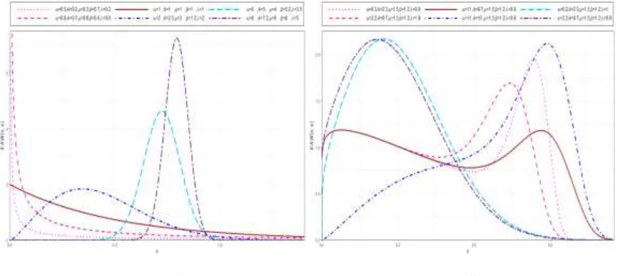
Figure 1 provides some plots of the density curves for different values of the parameters

𝛼, 𝜃, 𝜇, 𝛽 and 𝜆.

(𝑎) (𝑏)

Figure 1: Plots of the 𝑬𝑨𝑾 distribution for some parameter values.

(𝑎) (𝑏)

Figure 2: The 𝑬𝑨𝑾 hazard rate function for some parameter values.

It is known, not many lifetime distributions exhibit bathtub hazard rates. The 𝐸𝐴𝑊 model shows flexibility in accommodating all forms of the hazard rate function as seen from Figure 2 (by changing its parameter values) seems to be an important distribution that can be used.

2.1. Special Cases of the 𝑬𝑨𝑾 Distribution

𝐴 = Additive; 𝐺 = Generalized; 𝑀 = Modified, 𝑊 = Weibull, 𝐸_𝑥 = Exponential,

𝐸 =Exponentiated, 𝐿𝐹𝑅 = Linear Failure Rate and 𝑅 = Rayleigh. If 𝑋 is a random variable with cdf (3), then we have the following cases:

Table 1: The sub-models of the 𝑬𝑨𝑾 distribution

𝑴𝒐𝒅𝒆𝒍 𝛼 𝜃 𝜇 𝛽 𝜆 𝑪𝑫𝑭 References

𝐴𝑊 − − − − 1 1 − 𝑒−(𝛼𝑥𝜃+𝜇𝑥𝛽) Xie and Lai (1995)

𝐸𝑀𝑊 − 1 − − − [1 − 𝑒−(𝛼𝑥+𝜇𝑥𝛽)]𝜆 Elbatal (2011)

𝑀𝑊 − 1 − − 1 _{1 − 𝑒}−(𝛼𝑥+𝜇𝑥𝛽) Sarhan and Zaindin (2009)

𝐸𝑊 0 − − − − [1 − 𝑒−𝜇𝑥𝛽]𝜆 Mudholkar and Srivastava (1993)

𝐺𝐸_𝑥(𝐸𝐸_𝑥) − 1 0 − − [1 − 𝑒−𝛼𝑥]𝜆 Gupta and Kundu (1999)

𝐺𝑅 0 − − 2 − _{[1 − 𝑒}−𝜇𝑥2)_]𝜆 Kundu and Raqab (2005)

𝐺𝐿𝐹𝑅 − 1 − 2 − _{[1 − 𝑒}−(𝛼𝑥+𝜇𝑥2)_]𝜆 Sarhan and Kundu (2009)

𝐿𝐹𝑅 − 1 − 2 1 1 − 𝑒−(𝛼𝑥+𝜇𝑥2) Bain (1974)

𝑊 0 − − − 1 _{1 − 𝑒}−𝜇𝑥𝛽 Weibull (1951)

𝐸_𝑥 − 1 0 − 1 1 − 𝑒−𝛼𝑥 Bain (1974)

𝑅 0 − − 2 1 1 − 𝑒−𝜇𝑥2 Bain (1974)

3. Statistical Properties

In this section we studied the shapes, statistical properties, specifically moments, incomplete moment, and moment generating function of the (𝐸𝐴𝑊) distribution.

3.1. Shapes

We provide the shapes of the 𝐸𝐴𝑊 density function (4) and the shapes of the 𝐸𝐴𝑊 failure rate function (6). After some mathematical proccess, the limit of the pdf (4) as 𝑥 approaches to 0, is

lim

𝑥→0𝑓(𝑥) =

{

0, 𝜆 > 1, ∞, 0 < 𝜆 < 1, ∞, 0 < 𝜃 < 𝛽 < 1 or 0 < 𝛽 < 𝜃 < 1, 𝜆 = 1, ∞, 𝜃 > 1, 𝛽 < 1 or 𝜃 < 1, 𝛽 > 1, 𝜆 = 1, 0, 1 < 𝜃 < 𝛽 < ∞ or 1 < 𝛽 < 𝜃 < ∞, 𝜆 = 1, 𝛼 + 𝜇, 𝜃 = 𝛽 = 𝜆 = 1.

and the limit of the pdf (4) as 𝑥 approaches to ∞, is lim

3.2. Moments

In this section, the different moments of the exponentiated additive Weibull distribution can be obtained using the 𝑟𝑡ℎ moment 𝜇_𝑟′ = 𝐸(𝑋𝑟) and the moment generating function,

𝑀(𝑡) = 𝑒𝑡𝑋_.

Theorem 1 The 𝑟𝑡ℎ moment of 𝐸𝐴𝑊 distribution, 𝑟 = 1,2, . ... is given by

𝜇_𝑟′ _{= 𝜆 ∑}∞

𝑗,𝑘=0 (𝜆−1_𝑗 ) (−1)𝑗+𝑘 [𝜇(𝑗+1)] 𝑘

𝑘! [

𝛼Γ(𝑟+𝛽𝑘_𝜃 +1) [𝛼(𝑗+1)]𝑟+𝛽𝑘𝜃 +1

+ 𝜇𝛽Γ(

𝑟+𝛽(𝑘+1)

𝜃 )

𝜃[𝛼(𝑗+1)]𝑟+𝛽(𝑘+1)𝜃

] (8)

Proof We start with the well known definition of the 𝑟𝑡ℎ moment of the random variable

𝑋 with probability density function 𝑓(𝑥) given by

𝜇𝑟′ = ∫ ∞

0

𝑥𝑟_{𝑓(𝑥, 𝛼, 𝛽, 𝜆, 𝜃)𝑑𝑥.}

Substituting from (4) into the above relation, we get

𝜇_𝑟′ _{= 𝜆 ∫}∞ 0

𝑥𝑟_{(𝛼𝜃𝑥}𝜃−1_{+ 𝜇𝛽𝑥}𝛽−1_)𝑒−(𝛼𝑥𝜃+𝜇𝑥𝛽)_{[1 − 𝑒}−(𝛼𝑥𝜃+𝜇𝑥𝛽)_]𝜆−1_{𝑑𝑥, (9)}

since 0 < 𝑒−(𝛼𝑥𝜃+𝜇𝑥𝛽) < 1 for 𝑥 > 0, then by using the binomial series expansion of

[1 − 𝑒−(𝛼𝑥𝜃_+𝜇𝑥𝛽₎

]𝜆−1is given by

[1 − 𝑒−(𝛼𝑥𝜃_+𝜇𝑥𝛽₎

]𝜆−1 = ∑∞

𝑗=0(

𝜆 − 1

𝑗 ) (−1)𝑗𝑒−𝑗(𝛼𝑥

𝜃_+𝜇𝑥𝛽₎

, (10)

we get

𝜇_𝑟′ _{= 𝜆 ∑}∞ 𝑗=0(

𝜆 − 1

𝑗 ) (−1)𝑗∫

∞

0

(𝛼𝜃𝑥𝑟+𝜃−1_{+ 𝜇𝛽𝑥}𝑟+𝛽−1_)𝑒−(𝑗+1)(𝛼𝑥𝜃+𝜇𝑥𝛽)_{𝑑𝑥, (11)}

but the series expansion of 𝑒−(𝑗+1)𝜇𝑥𝛽 is given by

𝑒−(𝑗+1)𝜇𝑥𝛽 _{= ∑}∞ 𝑘=0

[−𝜇(𝑗 + 1)𝑥𝛽_]𝑘

𝑘! , (12)

substituting from (12) into (11), we get

𝜇_𝑟′ _{= 𝐶} 𝑗,𝑘∫

∞

0

(𝛼𝜃𝑥𝑟+𝛽𝑘+𝜃−1_{+ 𝜇𝛽𝑥}𝑟+𝛽(𝑘+1)−1_)𝑒−(𝑗+1)𝛼𝑥𝜃_{𝑑𝑥, (13)}

where

𝐶_𝑗,𝑘 = 𝜆 ∑∞

𝑗,𝑘=0(

𝜆 − 1

𝑗 ) (−1)𝑗+𝑘

[𝜇(𝑗 + 1)]𝑘

𝑘! ,

setting 𝑡 = (𝑗 + 1)𝛼𝑥𝜃, after some algebra, the integral in (13) can be computed as follows

𝜇𝑟′ = 𝐶𝑗,𝑘[

𝛼Γ(𝑟+𝛽𝑘_𝜃 + 1)

[𝛼(𝑗 + 1)]𝑟+𝛽𝑘𝜃 +1

+ 𝜇𝛽Γ(

𝑟+𝛽(𝑘+1)

𝜃 )

𝜃[𝛼(𝑗 + 1)]𝑟+𝛽(𝑘+1)𝜃

], (14)

The central moments 𝜇_𝑟 and cumulants 𝜅_𝑟 of the 𝐸𝐴𝑊 distribution can be determined from expression (8) as 𝜇_𝑟 = ∑𝑟_𝑚=0 (_𝑚𝑟)(−1)𝑚(𝜇₁′)𝑚𝜇_𝑟−𝑚′ and 𝜅_𝑟 = 𝜇_𝑟′ −

∑𝑟−1

𝑚=1 (_𝑚−1𝑟−1)𝜅𝑚 𝜇𝑟−𝑚′ , respectively, where 𝜅1 = 𝜇1 ′

, 𝜅₂ = 𝜇₂′ − (𝜇₁′)2, 𝜅₃ = 𝜇₃′ − 3𝜇₂′

𝜇₁′ + 2(𝜇₁′₎3_{, and 𝜅}

4 = 𝜇4′ − 4𝜇1′𝜇3 ′

− 3(𝜇₂′₎2_{+ 12𝜇} 2 ′_(𝜇

1′)2− 6(𝜇1′)4, etc. Additionally, the skewness and kurtosis can be calculated from the third and fourth standardized cumulants in the forms 𝑆𝐾 = 𝜅₃/√𝜅₂3 and 𝐾𝑈 = 𝜅₄/𝜅₂2, respectively.

Theorem 2 The moment generating function of 𝐸𝐴𝑊 distribution is given by

𝑀𝑋(𝑡) = ∑∞𝑗,𝑘,𝑟=0 𝑡 𝑟 𝑟!𝜆 (

𝜆−1

𝑗 ) (−1)𝑗+𝑘 [𝜇(𝑗+1)] 𝑘 𝑘! [

𝛼Γ(𝑟+𝛽𝑘_𝜃 +1)

[𝛼(𝑗+1)]𝑟+𝛽𝑘𝜃 +1

+ 𝜇𝛽Γ(

𝑟+𝛽(𝑘+1)

𝜃 )

𝜃[𝛼(𝑗+1)]𝑟+𝛽(𝑘+1)𝜃

]. (15)

Proof We start with the well known definition of the moment generating function given by 𝑀_𝑋(𝑡) = 𝐸(𝑒𝑡𝑋_{) = ∫}∞

0 𝑒𝑡𝑥𝑓𝐸𝐴𝑊(𝑥, 𝝓)𝑑𝑥, since ∑∞𝑟=0 𝑡𝑟 𝑟!𝑥

𝑟_{𝑓(𝑥) converges and each}

term is integrable for all 𝑡 close to 0, then we can rewrite the moment generating function as 𝑀_𝑋(𝑡) = ∑∞_𝑟=0 𝑡

𝑟 𝑟!𝐸(𝑋

𝑟_{) by replacing 𝐸(𝑋}𝑟_{). Hence using (8) the MGF of}

𝐸𝐴𝑊 distribution is given by

𝑀_𝑋(𝑡) = ∑∞ 𝑗,𝑘,𝑟=0𝑡

𝑟 𝑟!𝜆 (

𝜆−1

𝑗 ) (−1)𝑗+𝑘 [𝜇(𝑗+1)] 𝑘 𝑘! [

𝛼Γ(𝑟+𝛽𝑘_𝜃 +1)

[𝛼(𝑗+1)]𝑟+𝛽𝑘𝜃 +1

+ 𝜇𝛽Γ(

𝑟+𝛽(𝑘+1)

𝜃 )

𝜃[𝛼(𝑗+1)]𝑟+𝛽(𝑘+1)𝜃

].

which completes the proof.

Similarly, the characteristic function of the 𝐸𝐴𝑊 distribution becomes 𝜙_𝑋(𝑡) = 𝑀_𝑋(𝑖𝑡) where 𝑖 = √−1 is the unit imaginary number.

3.3. Conditional Moments

The main application of the first incomplete moment refers to the Bonferroni and Lorenz curves. These curves are very useful in economics, reliability, demography, insurance and medicine. The answers to many important questions in economics require more than just knowing the mean of the distribution, but its shape as well. This is obvious not only in the study of econometrics but in other areas as well. For lifetime models, it is also of interest to find the conditional moments and the mean residual lifetime function. The conditional moments for 𝐸𝐴𝑊 distribution is given by

𝜐_𝑠 = 𝐸(𝑋𝑠_{|𝑋 > 𝑡) = ∫}∞ 𝑡

𝑥𝑠_𝑓

𝐸𝐴𝑊(𝑥, 𝝓)𝑑𝑥.

= 𝐶_𝑗,𝑘∫∞

𝑡

(𝛼𝜃𝑥𝑠+𝛽𝑘+𝜃−1_{+ 𝜇𝛽𝑥}𝑠+𝛽(𝑘+1)−1_)𝑒−(𝑗+1)𝛼𝑥𝜃

𝑑𝑥.

= 𝐶𝑗,𝑘[

𝛼Γ(𝑠+𝛽𝑘_𝜃 + 1, (𝑗 + 1)𝛼𝑡𝜃₎

[𝛼(𝑗 + 1)]𝑠+𝛽𝑘𝜃 +1

+𝜇𝛽Γ(

𝑠+𝛽(𝑘+1)

𝜃 , (𝑗 + 1)𝛼𝑡

𝜃₎

𝜃[𝛼(𝑗 + 1)]𝑠+𝛽(𝑘+1)𝜃

]. (16)

where Γ(𝑠, 𝑡) = ∫_𝑡∞ 𝑥𝑠−1𝑒−𝑥𝑑𝑥 is the upper incomplete gamma function. The mean residual lifetime function is given by

𝜇(𝑡) = 𝐸(𝑋|𝑋 > 𝑡) − 𝑡 = 𝐶_𝑗,𝑘[𝛼Γ( 𝛽𝑘+1

𝜃 +1,(𝑗+1)𝛼𝑡𝜃)

[𝛼(𝑗+1)]𝑠+𝛽𝑘𝜃 +1

+𝜇𝛽Γ( 𝛽(𝑘+1)+1

𝜃 ,(𝑗+1)𝛼𝑡𝜃)

𝜃[𝛼(𝑗+1)]𝑠+𝛽(𝑘+1)𝜃

3.4. Quantile Function

The quantile function (qf) of 𝑋 is obtained by inverting (3), but there is no colsed form for the qf of 𝐸𝐴𝑊 distribtion. The 𝑝𝑡ℎ quantail of the 𝐸𝐴𝑊 distribtion can be obtained by numerically solving the following equaiton for 𝑥

ln (1 − 𝑝1𝜆) + 𝛼𝑥𝜃+ 𝜇𝑥𝛽 = 0. (18)

One can simulate the 𝐸𝐴𝑊 random variable with 𝝓 = (𝛼 , 𝜃,𝜇, 𝛽, 𝜆)𝑇 by: 1. Generate 𝑈~𝑛𝑢𝑖𝑓𝑜𝑟𝑚(0,1).

2. Put 𝑝 = 𝑈 in equation (18).

3. Solve equation (18) numerically for 𝑥.

The median can be calculated by putting 𝒑 = 𝟎. 𝟓 in equation (18), and solving it numerically for 𝒙.

4. Residual life and Reversed Failure Rate Function

Given that a component survives up to time 𝑡 ≥ 0, the residual life is the period beyond t until the time of failure and defined by the conditional random variable 𝑋 − 𝑡|𝑋 > 𝑡. In reliability, it is well known that the mean residual life function and ratio of two consecutive moments of residual life determine the distribution uniquely (Gupta and Gupta, 1983). Therefore, we obtain the 𝑟𝑡ℎ order moment of the residual lifetime can be obtained via the general formula

𝜇_𝑟(𝑡) = 𝐸((𝑋 − 𝑡)𝑟_{|𝑋 > 𝑡) =} 1

𝐹(𝑡)∫

∞

𝑡

(𝑥 − 𝑡)𝑟_{𝑓(𝑥, 𝜙)𝑑𝑥, 𝑟 ≥ 1.}

Applying the binomial expansion of (𝑥 − 𝑡)𝑟 into the above formula, we get

𝜇_𝑟(𝑡) = 1 𝐹(𝑡)∑

𝑟

𝑑=0

(−𝑡)𝑑₍𝑟

𝑑) ∫

∞

𝑡

𝑥𝑟−𝑑_{𝑓(𝑥)𝑑𝑥.}

= 𝐶𝑗,𝑘 𝐹(𝑡)∑

𝑟

𝑑=0

(−𝑡)𝑑₍𝑟

𝑑) ∫

∞

𝑡

(𝛼𝜃𝑥𝑟+𝛽𝑘+𝜃−𝑑−1_{+ 𝜇𝛽𝑥}𝑟+𝛽(𝑘+1)−𝑑−1_)𝑒−(𝑗+1)𝛼𝑥𝜃

𝑑𝑥.

=_𝐹(𝑡)𝐶𝑗,𝑘∑𝑟

𝑑=0 (−𝑡)𝑑(𝑟_{𝑑) [}

𝛼Γ(𝑟+𝛽𝑘−𝑑_𝜃 +1,(𝑗+1)𝛼𝑡𝜃)

[𝛼(𝑗+1)]𝑟+𝛽𝑘−𝑑𝜃 +1

+𝜇𝛽Γ(

𝑟+𝛽(𝑘+1)−𝑑

𝜃 ,(𝑗+1)𝛼𝑡𝜃) 𝜃[𝛼(𝑗+1)]𝑟+𝛽(𝑘+1)−𝑑𝜃

]. (19)

The mean residual life (MRL) of the 𝐸𝐴𝑊 distribution is given by

𝜇(𝑡) = 𝐶𝑗,𝑘 𝐹(𝑡)[

𝛼Γ (𝛽𝑘+1_𝜃 + 1, (𝑗 + 1)𝛼𝑡𝜃₎

[𝛼(𝑗 + 1)]𝛽𝑘+1𝜃 +1

+𝜇𝛽Γ (

𝛽(𝑘+1)+1

𝜃 , (𝑗 + 1)𝛼𝑡 𝜃₎

𝜃[𝛼(𝑗 + 1)]𝛽(𝑘+1)+1𝜃

] − 𝑡.

The variance of the residual life of the 𝐸𝐴𝑊 distribution can be obtained easily by using

On the other hand, we analogously discuss the reversed residual life and some of its properties. The reversed residual life can be defined as the conditional random variable

𝑡 − 𝑋|𝑋 ≤ 𝑡 which denotes the time elapsed from the failure of a component given that its life is less than or equal to 𝑡. This random variable may also be called the inactivity time (or time since failure); for more details you may see (Kundu and Nanda, 2010).

Also, in reliability, the mean reversed residual life and ratio of two consecutive moments of reversed residual life characterize the distribution uniquely. The reversed failure (or reversed hazard) rate function is given by Equation (7). The 𝑟𝑡ℎ order moment of the reversed residual life can be obtained by the well known formula

𝑚_𝑟(𝑡) = 𝐸((𝑡 − 𝑋)𝑟_{|𝑋 ≤ 𝑡) =} 1

𝐹(𝑡)∫

𝑡

0

(𝑡 − 𝑥)𝑟_{𝑓(𝑥, 𝜙)𝑑𝑥, 𝑟 ≥ 1.}

Applying the binomial expansion of (𝑡 − 𝑥)𝑟 into the above formula gives

𝑚_𝑟(𝑡) =𝑤𝑖,𝑗,𝑘 𝐹(𝑡) ∑

𝑟

𝑑=0

(−𝑡)𝑑₍𝑟

𝑑) ∫

𝑡

0

(𝛼𝜃𝑥𝑟+𝛽𝑘+𝜃−𝑑−1_{+ 𝜇𝛽𝑥}𝑟+𝛽(𝑘+1)−𝑑−1_)𝑒−(𝑗+1)𝛼𝑥𝜃

𝑑𝑥.

= 𝐶𝑗,𝑘 𝐹(𝑡)∑

𝑟

𝑑=0 (−𝑡)𝑑(𝑟_{𝑑) [}

𝛼𝜁(𝑟+𝛽𝑘−𝑑_𝜃 +1,(𝑗+1)𝛼𝑡𝜃)

[𝛼(𝑗+1)]𝑟+𝛽𝑘−𝑑𝜃 +1

+𝜇𝛽𝜁(

𝑟+𝛽(𝑘+1)−𝑑

𝜃 ,(𝑗+1)𝛼𝑡𝜃) 𝜃[𝛼(𝑗+1)]𝑟+𝛽(𝑘+1)−𝑑𝜃

]. (20)

where 𝜁(𝑠, 𝑡) = ∫₀𝑡 𝑥𝑠−1𝑒−𝑥𝑑𝑥 is the lower incomplete gamma function. Thus, the mean of the reversed residual life of the 𝐸𝐴𝑊 distribution is given by

𝑚(𝑡) = 𝑡 − 𝐶𝑗,𝑘 𝐹(𝑡)[

𝛼𝜁 (𝛽𝑘+1_𝜃 + 1, (𝑗 + 1)𝛼𝑡𝜃₎

[𝛼(𝑗 + 1)]𝛽𝑘+1𝜃 +1

+𝜇𝛽𝜁 (

𝛽(𝑘+1)+1

𝜃 , (𝑗 + 1)𝛼𝑡𝜃)

𝜃[𝛼(𝑗 + 1)]𝛽(𝑘+1)+1𝜃

]. (21)

Using 𝑚(𝑡) and 𝑚₂(𝑡) one can obtain the variance and the coefficient of variation of the reversed residual life of the 𝐸𝐴𝑊 distribution.

4.1. Bonferroni and Lorenz Curves

In this subsection we proposed the Bonferroni and Lorenz Curves. The Bonferroni and Lorenz curves (Bonferroni, 1930) and the Bonferroni and Gini indices have applications not only in economics to study income and poverty, but also in other fields like reliability, demography, insurance and medicine. The Bonferroni and Lorenz curves are defined by

𝐵(𝑝) = 1 𝑝𝜇∫

𝑞

0

𝑥𝑓(𝑥)𝑑𝑥 =𝐶𝑗,𝑘 𝑝𝜇[

𝛼𝜁 (𝛽𝑘+1_𝜃 + 1, (𝑗 + 1)𝑞𝑡𝜃₎

[𝛼(𝑗 + 1)]𝛽𝑘+1𝜃 +1

+𝜇𝛽𝜁 (

𝛽(𝑘+1)+1

𝜃 , (𝑗 + 1)𝑞𝑡 𝜃₎

𝜃[𝛼(𝑗 + 1)]𝛽(𝑘+1)+1𝜃

] (22)

and

𝐿(𝑝) = 1 𝜇∫

𝑞

0 𝑥𝑓(𝑥)𝑑𝑥 = 𝐶𝑗,𝑘

𝜇 [

𝛼𝜁(𝛽𝑘+1_𝜃 +1,(𝑗+1)𝑞𝑡𝜃₎ [𝛼(𝑗+1)]𝛽𝑘+1𝜃 +1

+𝜇𝛽𝜁(

𝛽(𝑘+1)+1

𝜃 ,(𝑗+1)𝑞𝑡𝜃) 𝜃[𝛼(𝑗+1)]𝛽(𝑘+1)+1𝜃

]. (23)

4.2. Mean deviation

distribution function 𝐹(𝑥), mean 𝜇 = 𝐸(𝑋) and 𝑀 = Median (𝑋), the mean deviation about the mean and mean deviation about the median, are defined by

𝛿1(𝑥) = ∫ ∞

0

|𝑥 − 𝜇|𝑓(𝑥)𝑑𝑥 = 2𝜇𝐹(𝜇) − 2𝜇 + 2 ∫

∞

𝜇

𝑥𝑓(𝑥)𝑑𝑥

and

𝛿₂(𝑥) = ∫

∞

0

|𝑥 − 𝑀|𝑓(𝑥)𝑑𝑥 = 2𝑀𝐹(𝑀) − 𝑀 − 𝜇 + 2 ∫

∞

𝑀

𝑥𝑓(𝑥)𝑑𝑥

respectively, if 𝑋 is 𝐸𝐴𝑊 random variable then

∫∞

𝜇

𝑥𝑓(𝑥)𝑑𝑥 = 𝐶_𝑗,𝑘[𝛼Γ (

𝛽𝑘+1

𝜃 + 1, (𝑗 + 1)𝜇𝑡 𝜃₎

[𝛼(𝑗 + 1)]𝛽𝑘+1𝜃 +1

+𝜇𝛽Γ (

𝛽(𝑘+1)+1

𝜃 , (𝑗 + 1)𝜇𝑡 𝜃₎

𝜃[𝛼(𝑗 + 1)]𝛽(𝑘+1)+1𝜃

] (24)

and

∫∞

𝑀

𝑥𝑓(𝑥)𝑑𝑥 = 𝐶𝑗,𝑘[

𝛼Γ (𝛽𝑘+1_𝜃 + 1, (𝑗 + 1)𝑀𝑡𝜃₎

[𝛼(𝑗 + 1)]𝛽𝑘+1𝜃 +1

+𝜇𝛽Γ (

𝛽(𝑘+1)+1

𝜃 , (𝑗 + 1)𝑀𝑡𝜃)

𝜃[𝛼(𝑗 + 1)]𝛽(𝑘+1)+1𝜃

] , (25)

so that

𝛿₁(𝑥) = 2𝜇𝐹(𝜇) + 2𝐶_𝑗,𝑘[𝛼Γ (

𝛽𝑘+1

𝜃 + 1, (𝑗 + 1)𝜇𝑡

𝜃₎

[𝛼(𝑗 + 1)]𝛽𝑘+1𝜃 +1

+𝜇𝛽Γ (

𝛽(𝑘+1)+1

𝜃 , (𝑗 + 1)𝜇𝑡

𝜃₎

𝜃[𝛼(𝑗 + 1)]𝛽(𝑘+1)+1𝜃

] − 2𝜇

and

𝛿2(𝑥) = −𝜇 + 2𝐶𝑗,𝑘[

𝛼Γ (𝛽𝑘+1_𝜃 + 1, (𝑗 + 1)𝑀𝑡𝜃₎

[𝛼(𝑗 + 1)]𝛽𝑘+1𝜃 +1

+𝜇𝛽Γ (

𝛽(𝑘+1)+1

𝜃 , (𝑗 + 1)𝑀𝑡𝜃)

𝜃[𝛼(𝑗 + 1)]𝛽(𝑘+1)+1𝜃

].

5. Maximum Likelihood Estimation

Statistical inference can be carried out in three different ways: point estimation, interval estimation and hypothesis testing. Several approaches for parameter point estimation were proposed in the literature but the maximum likelihood method is the most commonly employed. The 𝑀𝐿𝐸𝑠 enjoy desirable properties and can be used when constructing confidence intervals and regions and also in test statistics. Here, we determine the maximum likelihood estimates (𝑀𝐿𝐸𝑠) of the parameters of the 𝐸𝐴𝑊 distribution from complete samples only. Let 𝑥₁, . . . , 𝑥_𝑛 be a random sample of size 𝑛 from the 𝐸𝐴𝑊 distribution given by (4). Let 𝝓 = (𝛼, 𝜃, 𝜇, 𝛽, 𝜆)𝑇 be 5 × 1 vector of parameters. The total log-likelihood function for 𝝓 is given by

ℓ_𝑛 = ℓ_𝑛(𝝓) = 𝑛log𝜆 + ∑𝑛

𝑖=1log(𝛼𝜃𝑥𝑖

𝜃−1_{+ 𝜇𝛽𝑥}

𝑖𝛽−1) − 𝛼 ∑ 𝑛

𝑖=1𝑥𝑖

𝜃_{− 𝜇 ∑}𝑛 𝑖=1𝑥𝑖

𝛽

+(𝜆 − 1) ∑𝑛

𝑖=1 log [1 − 𝑒−𝛼𝑥𝑖 𝜃_−𝜇𝑥

𝑖𝛽]. (26)

The log-likelihood can be maximized either directly by using the SAS program or R -language (2018) or by solving the nonlinear likelihood equations obtained by differentiating (26). The associated components of the score function 𝑈_𝑛(𝝓) =

∂ℓ_𝑛

∂𝛼 = ∑

𝑛

𝑖=1

𝜃𝑥_𝑖𝜃−1 𝛼𝜃𝑥_𝑖𝜃−1_{+ 𝜇𝛽𝑥}

𝑖𝛽−1 − ∑𝑛

𝑖=1𝑥𝑖

𝜃_{+ (𝜆 − 1) ∑}𝑛 𝑖=1

𝑥_𝑖𝜃_𝑒−𝛼𝑥𝜃_−𝜇𝑥𝛽 1 − 𝑒−𝛼𝑥𝜃_−𝜇𝑥𝛽,

∂ℓ𝑛

∂𝜃 = 𝛼 ∑

𝑛

𝑖=1

𝑥𝑖𝜃−1(𝜃 ln(𝑥𝑖) + 1)

𝛼𝜃𝑥_𝑖𝜃−1_{+ 𝜇𝛽𝑥} 𝑖

𝛽−1 − 𝛼 ∑ 𝑛

𝑖=1𝑥𝑖

𝜃_ln(𝑥

𝑖) + 𝛼(𝜆 − 1) ∑ 𝑛

𝑖=1

𝑥𝑖𝜃ln(𝑥𝑖) 𝑒−𝛼𝑥𝑖

𝜃_−𝜇𝑥 𝑖𝛽

1 − 𝑒−𝛼𝑥_𝑖𝜃−𝜇𝑥_𝑖𝛽 , ∂ℓ𝑛

∂𝜇 = ∑

𝑛

𝑖=1

𝛽𝑥_𝑖𝛽−1 𝛼𝜃𝑥_𝑖𝜃−1_{+ 𝜇𝛽𝑥}

𝑖

𝛽−1− ∑

𝑛

𝑖=1𝑥𝑖

𝛽 _{+ (𝜆 − 1) ∑}𝑛 𝑖=1

𝑥_𝑖𝛽𝑒−𝛼𝑥_𝑖𝜃−𝜇𝑥_𝑖𝛽 1 − 𝑒−𝛼𝑥𝑖𝜃−𝜇𝑥𝑖 𝛽, ∂ℓ𝑛

∂𝛽 = 𝜇 ∑ 𝑛

𝑖=1

𝑥_𝑖𝛽−1(𝛽 ln(𝑥_𝑖) + 1) 𝛼𝜃𝑥_𝑖𝜃−1_{+ 𝜇𝛽𝑥}

𝑖

𝛽−1 − 𝜇 ∑ 𝑛

𝑖=1𝑥𝑖

𝛽_ln(𝑥

𝑖) + 𝜇(𝜆 − 1) ∑ 𝑛

𝑖=1

𝑥_𝑖𝛽ln(𝑥_𝑖) 𝑒−𝛼𝑥_𝑖𝜃−𝜇𝑥_𝑖𝛽 1 − 𝑒−𝛼𝑥𝑖𝜃−𝜇𝑥𝑖𝛽 and ∂ℓ𝑛 ∂𝜆 = 𝑛 𝜆+ ∑ 𝑛

𝑖=1log [1 − 𝑒

−𝛼𝑥_𝑖𝜃−𝜇𝑥_𝑖𝛽_{]. (27)}

The maximum likelihood estimation (𝑀𝐿𝐸) of 𝝓, say 𝝓̂, is obtained by solving the nonlinear system 𝑈_𝑛(𝝓) = 0. These equations cannot be solved analytically, and statistical software can be used to solve them numerically via iterative methods. We can use iterative techniques such as a Newton–Raphson type algorithm to obtain the estimate

𝝓̂. For interval estimation and hypothesis tests on the model parameters, we require the information matrix. The 5 × 5 observed information matrix is given by

𝐼_𝑛(𝝓) = − ( 𝐼𝛼𝛼 𝐼_𝜃𝛼 𝐼_𝜇𝛼 𝐼𝛽𝛼 𝐼𝜆𝛼 𝐼𝛼𝜃 𝐼_𝜃𝜃 𝐼_𝜇𝜃 𝐼𝛽𝜃 𝐼𝜆𝜃 𝐼_𝛼𝜇 𝐼𝜃𝜇 𝐼_𝜇𝜇 𝐼𝛽𝜇 𝐼𝜆𝜇 𝐼𝛼𝛽 𝐼𝜃𝛽 𝐼_𝜇𝛽 𝐼𝛽𝛽 𝐼𝜆𝛽 𝐼𝛼𝜆 𝐼_𝜃𝜆 𝐼_𝜇𝜆 𝐼𝛽𝜆 𝐼𝜆𝜆) (28)

whose elements are given in the Appendix. Applying the usual large sample approximation, 𝑀𝐿𝐸 of 𝝓, i.e 𝝓̂ can be treated as being approximately 𝑁₅(𝝓, 𝐽_𝑛(𝝓)−1), where 𝐽𝑛(𝝓) = 𝐸[𝐼𝑛(𝝓)]. Under conditions that are fulfilled for parameters in the interior of the parameter space but not on the boundary, the asymptotic distribution of

√𝑛(𝝓̂ − 𝝓) is 𝑁₅(0, 𝐽(𝝓)−1), where 𝐽(𝝓) = lim_𝑛→∞𝑛−1𝐼_𝑛(𝝓) is the unit information matrix. This asymptotic behavior remains valid if 𝐽(𝝓) is replaced by the average sample information matrix evaluated at 𝝓̂, say 𝑛−1𝐼_𝑛(𝝓̂). The estimated asymptotic multivariate normal 𝑁₅(𝝓, 𝐼_𝑛(𝝓̂)−1) distribution of 𝝓̂ can be used to construct approximate confidence intervals for the parameters and for the hazard rate and survival functions. An

100(1 − 𝛾)% asymptotic confidence interval for each parameter 𝝓_𝑟 is given by

𝐴𝐶𝐼_𝑟 = (𝝓̂_𝑟− 𝑧𝛾

2√𝐼̂,𝑟𝑟 𝝓

̂_{𝑟+ 𝑧}𝛾 2√𝐼̂)𝑟𝑟

where 𝑧_𝛾 is the upper 100𝛾𝑡ℎ percentile of the standard normal distribution.

6. Simulation Study

To test the validating of the theoretical results in Section 5, we produced simulations by R statistical package, by generating 2,000 samples of sizes 𝑛 = {50,65,80,95,110,125,

0.5, 𝛽 = 0.8, 𝜆 = 1.0)𝑇_{. The average of absolute value of biases, |𝐵𝑖𝑎𝑠(𝝓}̂)| = 1

𝑁∑ |𝝓̂ − 𝝓| 𝑛

𝑖=1 , and the mean square error of the estimates, 𝑀𝑆𝐸(𝝓̂) =_𝑁1∑ (𝝓̂ − 𝝓) 2 𝑛

𝑖=1 ,

are computed.

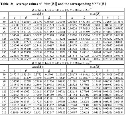
These results are reported in Table 2. We can see that the values of |𝐵𝑖𝑎𝑠(𝝓̂)| and

𝑀𝑆𝐸(𝝓̂) decrease as sample size increases.

Table 2: Average values of |𝐵𝑖𝑎𝑠(𝝓̂ )| and the corresponding 𝑀𝑆𝐸𝑠(𝝓̂ )

𝝓 = (𝛼 = 1.5, 𝜃 = 5.0, 𝜇 = 0.5, 𝛽 = 0.8, 𝜆 = 2.5)𝑇

𝑛 |𝐵𝑖𝑎𝑠(𝝓

̂)| 𝑀𝑆𝐸(𝝓̂)

𝛼̂ 𝜃̂ 𝜇̂ 𝛽̂ 𝜆̂ 𝛼̂ 𝜃̂ 𝜇̂ 𝛽̂ 𝜆̂

50 0.57616 4.29814 0.51799 0.86305 0.30088 0.55355 87.53188 0.49802 1.32654 0.14576 65 0.48383 3.09122 0.43974 0.73273 0.25280 0.42795 52.16778 0.39603 1.04794 0.10306 80 0.43713 2.52463 0.39121 0.65407 0.22458 0.36226 37.76243 0.32699 0.86033 0.07982 95 0.40471 2.13125 0.36282 0.61452 0.21061 0.31778 28.84269 0.28864 0.77003 0.07079 110 0.34544 1.49443 0.30870 0.52898 0.19748 0.23596 13.85096 0.21070 0.57212 0.06151 125 0.33062 1.44014 0.29469 0.50771 0.18231 0.22228 14.87032 0.19975 0.54232 0.05251 140 0.29282 1.11273 0.25848 0.45386 0.17255 0.18037 7.81345 0.15810 0.43699 0.04803 155 0.26793 0.92097 0.23486 0.40887 0.15943 0.14479 4.48580 0.12575 0.35057 0.04033 170 0.25577 0.85340 0.22479 0.40200 0.14981 0.13523 4.40740 0.11806 0.34442 0.03642 185 0.24217 0.73858 0.20989 0.37514 0.15079 0.11709 2.48610 0.09841 0.28683 0.03648 200 0.24137 0.78011 0.21059 0.37323 0.14123 0.11874 3.27028 0.10093 0.28895 0.03175 215 0.21879 0.64552 0.18912 0.34422 0.13317 0.09203 1.98047 0.07660 0.23179 0.02881

𝝓 = (𝛼 = 1.5, 𝜃 = 3.0, 𝜇 = 0.5, 𝛽 = 0.8, 𝜆 = 1.0)𝑇

𝑛

|𝐵𝑖𝑎𝑠(𝝓̂)| 𝑀𝑆𝐸(𝝓̂)

𝛼̂ 𝜃̂ 𝜇̂ 𝛽̂ 𝜆̂ 𝛼̂ 𝜃̂ 𝜇̂ 𝛽̂ 𝜆̂

50 0.47219 2.35138 0.3733 0.2904 0.12029 0.38673 44.14962 0.27557 0.14808 0.02723 65 0.40947 1.47379 0.31196 0.24059 0.10645 0.29333 15.98097 0.19662 0.10142 0.02247 80 0.34597 1.02278 0.27689 0.21726 0.09853 0.21681 6.30872 0.15462 0.08286 0.02118 95 0.31842 0.83252 0.25594 0.19913 0.09329 0.18324 3.57361 0.13048 0.06957 0.02142 110 0.2999 0.71863 0.23043 0.18095 0.08775 0.15585 3.38734 0.10583 0.05707 0.02222 125 0.26463 0.60621 0.21624 0.17205 0.08726 0.12614 1.77998 0.09061 0.05101 0.02493 140 0.24863 0.53581 0.19605 0.15689 0.08218 0.11054 1.25309 0.07441 0.04233 0.02265 155 0.24779 0.50124 0.19101 0.15191 0.0854 0.10649 0.81173 0.07087 0.04023 0.02901 170 0.22066 0.43431 0.17234 0.13991 0.07958 0.08586 0.62951 0.05631 0.03333 0.02445 185 0.21615 0.40192 0.16582 0.13332 0.07844 0.07963 0.39007 0.05227 0.03092 0.0258 200 0.20041 0.38007 0.15828 0.13092 0.07134 0.06799 0.31900 0.04586 0.02849 0.01999 215 0.1949 0.35905 0.1501 0.12247 0.07823 0.06487 0.29628 0.04112 0.02526 0.02834

7. Application

the smallest the values of 𝑊∗, 𝐴∗ and 𝐾 − 𝑆 statistics, and the largest 𝐾 − 𝑆 𝑝-value, is considered the best fit to the data. The required computations are carried out using the 𝑅 software.

The data used in this research is corresponding to remission times (in months) of a random sample of 128 bladder cancer patients given in Lee and Wang (2003). The data is given as follows:

0.08, 0.20, 0.40, 0.50, 0.51, 0.81, 0.90, 1.05, 1.19, 1.26, 1.35, 1.40, 1.46, 1.76, 2.02, 2.02, 2.07, 2.09, 2.23, 2.26, 2.46, 2.54, 2.62, 2.64, 2.69, 2.69, 2.75, 2.83, 2.87, 3.02, 3.25, 3.31, 3.36, 3.36, 3.48, 3.52, 3.57, 3.64, 3.70, 3.82, 3.88, 4.18, 4.23, 4.26, 4.33, 4.34, 4.40, 4.50, 4.51, 4.87, 4.98, 5.06, 5.09, 5.17, 5.32, 5.32, 5.34, 5.41, 5.41, 5.49, 5.62, 5.71, 5.85, 6.25, 6.54, 6.76, 6.93, 6.94, 6.97, 7.09, 7.26, 7.28, 7.32, 7.39, 7.59, 7.62, 7.63, 7.66, 7.87, 7.93, 8.26, 8.37, 8.53, 8.65, 8.66, 9.02, 9.22, 9.47, 9.74, 10.06, 10.34, 10.66, 10.75, 11.25, 11.64, 11.79, 11.98, 12.02, 12.03, 12.07, 12.63, 13.11, 13.29, 13.80, 14.24, 14.76, 14.77, 14.83, 15.96, 16.62, 17.12, 17.14, 17.36, 18.10, 19.13, 20.28, 21.73, 22.69, 23.63, 25.74, 25.82, 26.31, 32.15, 34.26, 36.66, 43.01, 46.12, 79.05.

Table 3: The statistics: −𝟐𝓵𝟏𝟐𝟖(𝝓̂),𝑾∗ and 𝑨∗ for the bladder cancer data

Model −2ℓ₁₂₈(𝝓̂) 𝑊∗ 𝐴∗ 𝐾 − 𝑆 𝑝-value 𝑬𝑨𝑾 819.746 0.0235 0.1523 0.0349 0.9976

𝑲𝒘 − 𝑴𝑾 821.504 0.0457 0.3007 0.0456 0.9530 𝑴𝑾 828.175 0.1314 0.7864 0.0700 0.5575 𝑾 828.174 0.1314 0.7865 0.0700 0.5570 𝑬𝑬_𝒙 826.155 0.1122 0.6741 0.0725 0.5113 𝑬_𝒙 828.684 0.1193 0.7160 0.0846 0.3184 𝑬𝑾 821.360 0.0437 0.2885 0.0450 0.9576

𝑹 982.531 0.4664 2.7300 0.3521 0.0000

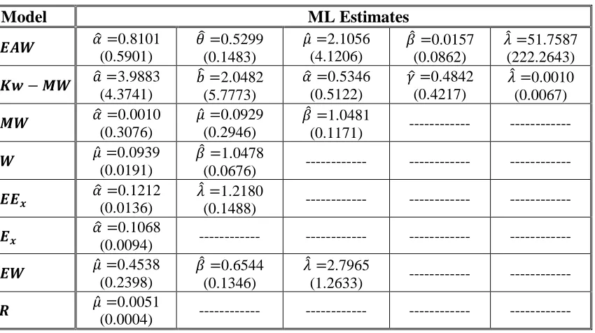
Table 4: 𝑴𝑳𝑬𝒔 and their standard errors (in parentheses) for the bladder cancer data

Model ML Estimates

𝑬𝑨𝑾 𝛼̂ =0.8101 (0.5901)

𝜃̂ =0.5299 (0.1483)

𝜇̂ =2.1056 (4.1206)

𝛽̂ =0.0157 (0.0862)

𝜆̂ =51.7587 (222.2643)

𝑲𝒘 − 𝑴𝑾 𝑎̂ =3.9883 (4.3741)

𝑏̂ =2.0482 (5.7773)

𝛼̂ =0.5346 (0.5122)

𝛾̂ =0.4842 (0.4217)

𝜆̂ =0.0010 (0.0067)

𝑴𝑾 𝛼̂ =0.0010 (0.3076)

𝜇̂ =0.0929 (0.2946)

𝛽̂ =1.0481

(0.1171) ---

---𝑾 𝜇̂ =0.0939 (0.0191)

𝛽̂ =1.0478

(0.0676) --- ---

---𝑬𝑬_𝒙 𝛼̂ =0.1212 (0.0136)

𝜆̂ =1.2180

(0.1488) --- ---

---𝑬_𝒙 𝛼̂ =0.1068

(0.0094) --- --- ---

---𝑬𝑾 𝜇̂ =0.4538 (0.2398)

𝛽̂ =0.6544 (0.1346)

𝜆̂ =2.7965

(1.2633) ---

𝑹 𝜇̂ =0.0051

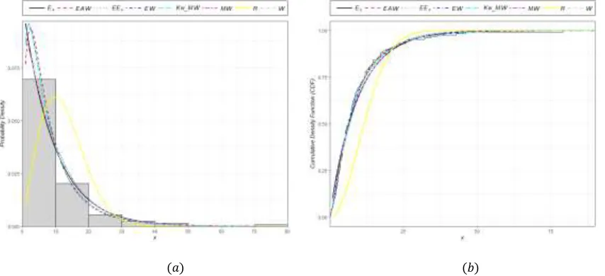
---Figure 3 displays: (𝑎) the estimated densities of the 𝐸𝐴𝑊, 𝐾𝑤 − 𝑀𝑊,𝑀𝑊,𝑊,𝐸𝐸, 𝐸,

𝐸𝑊, 𝐿 and 𝑅 distributions for the data, and (𝑏) the estimated cdf from the fitted the

𝐸𝐴𝑊, Kumaraswamy modified Weibull distribution (𝐾𝑤 − 𝑀𝑊) (Cordeiro et al., (2014)),𝑀𝑊, 𝑊, 𝐸𝐸_𝑥, 𝐸_𝑥, 𝐸𝑊 and 𝑅 distributions and the empirical cdf of the data set. These results indicate that the 𝐸𝐴𝑊 model has the lowest values of 𝑊∗, 𝐴∗ and 𝐾 − 𝑆 statistics and the largest 𝐾 − 𝑆 𝑝-value, among the fitted distributions, and therefore it could be chosen as the best model.

(𝑎) (𝑏)

Figure 3: The estimated densities (𝑎) and the estimated cdf (𝑏) of the 𝑬𝑨𝑾 distributionand other estimated distributions,for the bladder cancer data.

References

1. Bain L.J. (1974). Analysis for the linear failure -rate life- testing distribution. Technometrics; 16 (4): 551–9.

2. Bakouch, H. S., Al-Zahrani, B. M., Al-Shomrani, A, Marchi, V. A and Louzada, F. (2011). An extended lindley distribution. Journal of the Korean Statistical Society, 41(1): 75–85.

3. Barriga, G. D. C., Louzada, F. and Cancho, V. G. (2011). The Complementary Exponential Power lifetime model. Computational Statistics and Data Analysis, 54(5): 1250–1259.

4. Bebbington MS, Lai CD, and Zitikis, R. (2007). Aflexible Weibull extension. Reliability Engineering and System Safety. 92 (6), 719–26.

5. Bonferroni C.E. (1930). Elmenti di statistica generale. Libreria Seber, Firenze. 6. Choulakian, V., Stephens, MA. (2001). Goodness-of-fit for the generalized Pareto

distribution, Technometrics. 43 (4), 478-484.

8. Development Core Team, R. A. (2012). Language and Environment for Statistical Computing, R Foundation for Statistical Computing, Vienna, Austria.

9. Elbatal. I (2011) Exponentiated modified Weibull distribution. Economic Quality Control. 26, 189–200.

10. Gupta, P.L. and Gupta,R.C (1983). On the moments of residual life in reliability and some characterization results, Communications in Statistics-Theory and Methods, 12, 449–461.

11. Gupta, R.D, Kundu, D.(2001). Exponentiated exponential distribution. An alternative to gamma and Weibull distributions. Biometrical Journal 43, 117–130. 12. Kundu, C., Nanda, A. K. (2010). Some reliability properties of the inactivity time.

Communications in StatisticsTheory and Methods, 39, 899–911.

13. Lai, C.D, Xie, M, Murthy, D.N.P.(2003). A modified Weibull distribution. IEEE Transactions on Reliability 52, 33–37.

14. Lee, E. and Wang. J. (2003). Statistical methods for survival data analysis. 3. New York: Wiley.

15. Miller, J.R.G. (1981). Survival Analysis,Wiley,New York.

16. Mudholkar GS, Srivastava D K. (1993). Exponentiated Weibull family for analyzing bathtub failure- rate data. IEEETransactions on Reliability. 42(2): 299– 302.

17. Mudholkar G, Srivastava D, Kollia G. (1996) A Generalization of the Weibull Distribution with Application to the Analysis of Survival Data. Journal of the American Statistical Association. 91, 1575–1583.

18. Nadarajah, S. and Kotz, S. (2006). The exponentiated type distributions. Acta Applicandae Mathematicae, 92, 97–11.

19. Pham, H., Lai, C.D.(2007). On recent generalizations of the Weibull distribution. IEEE Transactions on Reliability 56, 454–458.

20. Sarhan, A and Kundu, D (2009) Generalized linear failure rate distribution, Commun. Statist. Theory Methods 38 (5), 642–660.

21. Sarhan A M, and Zaindin M. (2009). Modified Weibull distribution. Applied Sciences .11, 123 –36.

22. Smith, R. M. & Bain, L. J. (1975). An exponential power life-testing distribution. Communications in Statistics - Theory and Methods, 4, 469–481.

23. Weibull W. A. (1951). Statistical distribution function of wide applicability.Journal of Applied Mechanics. 18, 293–297.

24. Xie, M. and Lai, C. D. (1995). Reliability analysis using an additive Weibull model with bathtub-shaped failure rate function. Reliability Engineering and System Safety, 52, 87–93.

Appendix

Let 𝑆(𝑥) = 𝑒−(𝛼𝑥𝜃+𝜇𝑥𝛽), the entries of the matrix, 𝐼_𝑛(𝝓), in (28), are

𝐼𝛼𝛼=

∂2_ℓ 𝑛

∂𝛼2 = 𝜆(1 − 𝑆(𝑥)) 𝜆−3

𝑆(𝑥) 𝑥2𝜃−1_[(𝜃(𝑥𝜃_{𝛼 − 2) + 𝛽𝜇𝑥}𝛽_{) + 𝜆𝑆}2_{(𝑥)(𝜃(𝛼𝜆𝑥}𝜃_{− 2) + 𝛽𝜆𝜇𝑥}𝛽₎

+ 𝑆(𝑥) (𝜃 (2(1 + 𝜆) + 𝛼𝑥𝜃_{(1 − 3𝜆)) + 𝜇𝛽(1 − 3𝜆)𝑥}𝛽_)],

𝐼𝜃𝜃=

∂2_ℓ 𝑛

∂𝜃2 = 𝛼𝜆 (1 − 𝑆(𝑥)) 𝜆−3

log(𝑥)𝑆(𝑥)𝑥𝜃−1_{[2(1 − 𝑆(𝑥)) ((1 − 𝛼𝑥}𝜃_{) + 𝑆(𝑥)(𝛼𝜆𝑥}𝜃_{− 1))}

+ log(𝑥) (𝜃 [𝑆2_{(𝑥) + (1 + 𝛼𝑥}𝜃_(𝛼𝑥𝜃_{− 3)) + 𝛼𝜆𝑥}𝜃_𝑆2_{(𝑥)(𝛼𝜆𝑥}𝜃_{− 3)}

+ 𝑆(𝑥)(𝛼𝑥𝜃_{(3(𝜆 + 1) + 𝛼(1 − 3𝜆)𝑥}𝜃_{) − 2)]}

+ 𝛽𝜇𝑥𝛽_[(𝛼𝑥𝜃_{− 1) + 𝜆(𝛼𝜆𝑥}𝜃_{− 1) + 𝑆(𝑥)(1 + 𝜆 + 𝛼(1 − 3𝜆)𝑥}𝜃_)])],

𝐼𝜇𝜇=

∂2_ℓ 𝑛

∂𝜇2 = 𝜆(1 − 𝑆(𝑥)) 𝜆−3

𝑆(𝑥)𝑥2𝛽−1_{[(𝛽(𝜇𝑥}𝛽_{− 2) + 𝛼𝜃𝑥}𝜃_{) + 𝜆𝑆}2_{(𝑥)(𝛽(𝜆𝜇𝑥}𝛽_{− 2) + 𝛼𝜃𝜆𝑥}𝜃₎

+ 𝑆(𝑥) (𝛽 (2(1 + 𝜆) + 𝜇𝑥𝛽_{(1 − 3𝜆)) + 𝛼𝜃(1 − 3𝜆)𝑥}𝜃_)],

𝐼𝛽𝛽 =

∂2_ℓ 𝑛

∂𝛽2 = 𝜇𝜆 (1 − 𝑆(𝑥)) 𝜆−3

log(𝑥)𝑆(𝑥)𝑥𝛽−1_{[2(1 − 𝑆(𝑥)) ((1 − 𝜇𝑥}𝛽_{) + 𝑆(𝑥)(𝜇𝜆𝑥}𝛽_{− 1))}

+ log(𝑥) (𝛽 [𝑆2_{(𝑥) + (1 + 𝜇𝑥}𝛽_(𝜇𝑥𝛽_{− 3)) + 𝜇𝜆𝑥}𝛽_𝑆2_{(𝑥)(𝜇𝜆𝑥}𝛽_{− 3)}

+ 𝑆(𝑥)(𝜇𝑥𝛽_{(3(𝜆 + 1) + 𝜇(1 − 3𝜆)𝑥}𝛽_{) − 2)]}

+ 𝛼𝜃𝑥𝜃_[(𝜇𝑥𝛽_{− 1) + 𝜆(𝜇𝜆𝑥}𝛽_{− 1) + 𝑆(𝑥)(1 + 𝜆 + 𝜇(1 − 3𝜆)𝑥}𝛽_)])],

𝐼𝜆𝜆=

∂2_ℓ 𝑛

∂𝜆2 = 𝑆(𝑥)𝑥−1(1 − 𝑆(𝑥)) 𝜆−1

(𝛼𝜃𝑥𝜃_{+ 𝛽𝜇𝑥}𝛽_{) log(1 − 𝑆(𝑥)) (𝜆 log(1 − 𝑆(𝑥)) + 2),}

𝐼𝛼𝜃=

∂2_ℓ 𝑛

∂𝛼 ∂𝜃 = ∂2ℓ𝑛

∂𝜃 ∂𝛼= 𝜆𝑆(𝑥)(1 − 𝑆(𝑥))

𝜆−3

𝑥𝜃−1_{[(1 − 𝑆(𝑥)) ((1 − 𝛼𝑥}𝜃_{) + 𝑆(𝑥)(𝛼𝜆𝑥}𝜃_{− 1))}

+ log(𝑥) (𝜃 [𝑆2_{(𝑥) + (1 + 𝛼𝑥}𝜃_(𝛼𝑥𝜃_{− 3)) + 𝑆}2_{(𝑥)𝛼𝜆𝑥}𝜃_{(𝛼𝜆𝑥}𝜃_{− 3)}

+ 𝑆(𝑥) (𝛼𝑥𝜃_{(3(1 + 𝜆) + 𝛼𝑥}𝜃_{(1 − 3𝜆)) − 2)]}

+ 𝛽𝜇𝑥𝛽_[(𝛼𝑥𝜃_{− 1) + 𝜆𝑆}2_{(𝑥)(𝛼𝜆𝑥}𝜃_{− 1) + 𝑆(𝑥) (1 + 𝜆 + 𝛼𝑥}𝜃_{(1 − 3𝜆))])],}

𝐼𝛼𝜇=

∂2_ℓ 𝑛

∂𝛼 ∂𝜇 = ∂

2_ℓ 𝑛

∂𝜇 ∂𝛼= 𝑆(𝑥)(1 − 𝑆(𝑥))

𝜆−3

𝑥𝛽+𝜃−1_{𝜆 [((𝛼𝑥}𝜃_{− 1)𝜃 + 𝛽(−1 + 𝑥}𝛽_𝜇))

+ 𝑆(𝑥) (𝜃 (1 + 𝜆 + 𝑥𝜃_{𝛼(1 − 3𝜆)) + 𝛽 (1 + 𝜆 + 𝜇𝑥}𝛽_{(1 − 3𝜆)))}

+ 𝑆2_{(𝑥)𝜆 (𝜃(𝛼𝜆𝑥}𝜃_{− 1) + 𝛽(𝜆𝜇𝑥}𝛽_{− 1))],}

𝐼𝛼𝛽=

∂2_ℓ 𝑛

= ∂

2_ℓ 𝑛

∂𝛽 ∂𝛼= 𝜆𝜇𝑆(𝑥)(1 − 𝑆(𝑥))

𝜆−3

𝑥𝛽+𝜃−1_{[(1 − 𝑆(𝑥))(𝜆𝑆(𝑥) − 1)}

+ log(𝑥) ((𝜃(𝛼𝑥𝜃_{− 1) + 𝛽(𝜇𝑥}𝛽_{− 1))}

+ 𝑆(𝑥) (𝜃 (1 + 𝜆 + 𝛼𝑥𝜃_{(1 − 3𝜆)) + 𝛽 (1 + 𝜆 + 𝜇𝑥}𝛽_{(1 − 3𝜆)))}

+ 𝜆𝑆2_{(𝑥) (𝜃(𝛼𝜆𝑥}𝜃_{− 1) + 𝛽(𝜆𝜇𝑥}𝛽_{− 1)))],}

𝐼𝛼𝜆=

∂2_ℓ 𝑛

∂𝛼 ∂𝜆 = ∂

2_ℓ 𝑛

∂𝜆 ∂𝛼= −𝑆(𝑥)(1 − 𝑆(𝑥))

𝜆−2

𝑥𝜃−1_{[𝜃 (𝑆(𝑥) + (𝛼𝑥}𝜃_{− 1) − 2𝛼𝜆𝑥}𝜃_{𝑆(𝑥)) + 𝛽𝜇𝑥}𝛽_{(1 − 2𝜆𝑆(𝑥))}

− 𝜆 log(1 − 𝑆(𝑥)) (𝜃(𝛼𝑥𝜃_{(𝜆𝑆(𝑥) − 1) − 𝑆(𝑥) + 1) − 𝜇𝛽𝑥}𝛽_{(1 − 𝜆𝑆(𝑥)))],}

𝐼𝜃𝜇=

∂2_ℓ 𝑛

∂𝜃 ∂𝜇 = ∂2ℓ𝑛

∂𝜇 ∂𝜃= 𝛼𝜆𝑆(𝑥)(1 − 𝑆(𝑥))

𝜆−3

𝑥𝛽+𝜃−1_{[(1 − 𝑆(𝑥))(𝜆𝑆(𝑥) − 1)}

+ log(𝑥) ((𝜃(𝛼𝑥𝜃_{− 1) + 𝛽(𝜇𝑥}𝛽_{− 1))}

+ 𝑆(𝑥) (𝜃 (1 + 𝜆 + 𝛼𝑥𝜃_{(1 − 3𝜆)) + 𝛽 (1 + 𝜆 + 𝜇𝑥}𝛽_{(1 − 3𝜆)))}

+ 𝜆𝑆2_{(𝑥) (𝜃(𝛼𝜆𝑥}𝜃_{− 1) + 𝛽(𝜆𝜇𝑥}𝛽_{− 1)))],}

𝐼𝜇𝜆=

∂2_ℓ 𝑛

∂𝜇 ∂𝜆 = ∂

2_ℓ 𝑛

∂𝜆 ∂𝜇= −𝑆(𝑥)(1 − 𝑆(𝑥))

𝜆−2

𝑥𝛽−1_{[𝛼𝜃𝑥}𝜃_{(1 − 2𝜆𝑆(𝑥)) + 𝛽 (𝑆(𝑥)(1 − 2𝜆𝜇𝑥}𝛽_{) + (𝜇𝑥}𝛽_{− 1))}

+ 𝜆 log(1 − 𝑆(𝑥)) (𝑥𝜃_{𝛼𝜃(1 − 𝜆𝑆(𝑥)) − 𝛽 (𝑆(𝑥)(𝜆𝜇𝑥}𝛽_{− 1) + (1 − 𝜇𝑥}𝛽_)))],

𝐼𝜃𝛽=

∂2_ℓ 𝑛

∂𝜃 ∂𝛽 = ∂2ℓ𝑛

∂𝛽 ∂𝜃= 𝛼𝜆𝜇𝑆(𝑥)(1 − 𝑆(𝑥))

𝜆−1

log(𝑥) 𝑥𝛽+𝜃−1_{[2(1 − 𝑆(𝑥))(𝜆𝑆(𝑥) − 1)}

+ log(𝑥) ((𝜃(𝛼𝑥𝜃_{− 1) + 𝛽(𝜇𝑥}𝛽_{− 1))}

+ 𝑆(𝑥) (𝜃 (1 + 𝜆 + 𝛼𝑥𝜃_{(1 − 3𝜆)) + 𝛽 (1 + 𝜆 + 𝜇𝑥}𝛽_{(1 − 3𝜆)))}

+ 𝜆𝑆2_{(𝑥) (𝜃(𝛼𝜆𝑥}𝜃_{− 1) + 𝛽(𝜆𝜇𝑥}𝛽_{− 1)))],}

𝐼𝜃𝜆=

∂2_ℓ 𝑛

= ∂

2_ℓ 𝑛

∂𝜆 ∂𝜃= 𝛼𝑆(𝑥)(1 − 𝑆(𝑥))

𝜆−2

𝑥𝜃−1_{[1 − 𝑆(𝑥)(𝜃 log(𝑥) + 1)}

+ log(𝑥) ((𝜃(1 − 𝛼𝑥𝜃_{) − 𝛽𝜇𝑥}𝛽_{) + 2𝜆𝑆(𝑥)(𝛼𝜃𝑥}𝜃_{+ 𝛽𝜇𝑥}𝛽₎₎

+ 𝜆 log(1 − 𝑆(𝑥)) (1 − 𝑆(𝑥)

+ log(𝑥) (𝜃 ((1 − 𝛼𝑥𝜃_{) + 𝑆(𝑥)(𝛼𝜆𝑥}𝜃_{− 1)) − 𝜇𝛽𝑥}𝛽_{(1 − 𝜆𝑆(𝑥))))],}

𝐼𝜇𝛽=

∂2_ℓ 𝑛

∂𝜇 ∂𝛽 = ∂

2_ℓ 𝑛

∂𝛽 ∂𝜇= 𝜆𝑆(𝑥)(1 − 𝑆(𝑥))

𝜆−3

𝑥𝛽−1_{[(1 − 𝑆(𝑥)) (𝑆(𝑥)(𝜆𝜇𝑥}𝛽_{− 1) + (1 − 𝜇𝑥}𝛽₎₎

+ log(𝑥) (𝛼𝜃𝑥𝜃_((𝜇𝑥𝛽_{− 1) + 𝑆(𝑥) (1 + 𝜆 + 𝜇𝑥}𝛽_{(1 − 3𝜆)) + 𝑆}2_{(𝑥)𝜆(𝜆𝜇𝑥}𝛽_{− 1))}

+ 𝛽 (𝑆2_{(𝑥) (1 + 𝜆𝜇𝑥}𝛽_{(𝜆𝜇𝑥}𝛽_{− 3)) + (1 + 𝑥}𝛽_{𝜇(𝜇𝑥}𝛽_{− 3))}

+ 𝑆(𝑥) (𝜇𝑥𝛽_{(3(1 + 𝜆) + 𝜇𝑥}𝛽_{(1 − 3𝜆)) − 2)))],}

and

𝐼𝛽𝜆=

∂2_ℓ 𝑛

∂𝛽 ∂𝜆 = ∂2ℓ𝑛

∂𝜆 ∂𝛽= 𝜇𝑆(𝑥)(1 − 𝑆(𝑥))

𝜆−2

𝑥𝛽−1_{[1 − 𝑆(𝑥)(𝛽Log[𝑥] + 1)}

+ log(𝑥) ((𝛽(1 − 𝜇𝑥𝛽_{) − 𝛼𝜃𝑥}𝜃_{) + 2𝜆𝑆(𝑥)(𝛼𝜃𝑥}𝜃_{+ 𝛽𝜇𝑥}𝛽₎₎

+ 𝜆 log(1 − 𝑆(𝑥)) (1 − 𝑆(𝑥)