Sensitive Variable Using Optional Randomized Response Technique
Lovleen Kumar Grover Department of Mathematics,
Guru Nanak Dev University, Amritsar, Punjab, India Email:[email protected]
Amanpreet Kaur
Department of Mathematics,
Guru Nanak Dev University, Amritsar, Punjab, India
Abstract
In this paper, we improve the efficiency of Koyuncu et al (2014)’s estimator of population mean of sensitive variable by replacing Traditional Randomized response technique with Optional Randomized response technique as suggested by Gupta et al (2014). The mean square error of proposed estimator is obtained, up to first order of approximation, and is compared with mean square error of various existing estimators theoretically as well as numerically.
Keywords: Auxiliary variable; bias; efficiency; mean square error; randomized response technique; simple random sampling without replacement; sensitive study variable; percent relative efficiency.
AMS Classification: 62D05
1.
Introductionwhereas some authors in the literature like Singh and Tarray (2014), Tarray et al (2015), etc studied optional randomized response model for qualitative study variable. To support theoretical results obtained, a numerical illustration is considered finally.
2.
Notations and existing estimatorsConsider a population 𝑈 = (𝑈1, 𝑈2, … , 𝑈𝑁) of size N from which a sample of size 𝑛 is drawn using simple random sampling without replacement. Let 𝑌 be the study variable which is sensitive in nature. Let 𝑋 be a non-sensitive auxiliary variable which is positively correlated with the study variable 𝑌. Let 𝑊 be the sensitivity level of the asked sensitive question. The respondent gives the correct response for the auxiliary variable
𝑋 but has optional randomized response for variable 𝑌. In this Optional RRT model, respondent gives the response as Ƶ = 𝑌 + 𝑆𝑇 for the study variable 𝑌, where T is a Bernoulli random variable with parameter 𝑊, so that 0 ≤ 𝑊 ≤ 1 and 𝑆 is a scrambling variable whose mean is assumed to be zero i.e. 𝐸(𝑆) = 𝑆̅ = 0 and its variance 𝜎𝑠2 is assumed to be known quantity. It is assumed that the variables 𝑆 and 𝑇 are two mutually independent variables which are further independent of variables 𝑌 and 𝑋.
Remark 2.1:
If we take 𝑊 = 1 in the above model then it reduces to the traditional additive RRT model, and scrambled response is then written as 𝑍 = 𝑌 + 𝑆.
Now the population mean of variable Ƶ is given by Ƶ̅ = 𝐸(Ƶ) = 𝐸(𝑌 + 𝑆𝑇) = 𝐸(𝑌) =
𝑌̅ = 𝜇𝑌Ƶ(say) as 𝐸(𝑆) = 0, where 𝑌̅ is the population mean of variable 𝑌. The population
variance of variable Ƶ is given by 𝑆ƶ2 = 𝑉(𝑌 + 𝑆𝑇) = 𝑆𝑦2+ 𝑊𝑆𝑠2. Let 𝐶ƶ be the
coefficient of variation of variable Ƶ. So 𝐶ƶ2 = 𝐶𝑦2+ 𝑊𝑆𝑠 2
𝑌̅2, where 𝐶𝑦 is the coefficient of variation of variable 𝑌. Let 𝜌ƶ𝑥 be the coefficient of correlation between variables Ƶ and
𝑋 so 𝜌ƶ𝑥 = 𝜌𝑦𝑥
√1+𝑊𝑆𝑠2
𝑆𝑦2
, where 𝜌𝑦𝑥 is the coefficient of correlation between variables 𝑌 and
𝑋, 𝑆𝑦2 =𝑁−11 ∑𝑁𝑖=1(𝑦𝑖 − 𝑌̅)2, and 𝑆𝑠2 =𝑁−11 ∑𝑁𝑖=1(𝑠𝑖 − 𝑆̅)2.
Taking also 𝑆𝑥2 =𝑁−11 ∑𝑁𝑖=1(𝑥𝑖 − 𝑋̅)2, where 𝑋̅ is the population mean of auxiliary variable 𝑋. Let 𝐶𝑥 be the coefficient of variation of variable 𝑋.
Remark 2.2:
The estimate of sensitivity level 𝑊 in the above Optional RRT model may be obtained by using the same approach of Gupta et al (2014). According to them, the estimated value of
𝑊 is 𝑊̂ = 1
𝑛∑ ƶ𝑖2−{𝑉̂(𝑦)+(
1 𝑛∑𝑛𝑖=1ƶ𝑖)
2
}
𝑛 𝑖=1
𝐸(𝑠2) , where 𝑉̂(𝑦) is the estimate of variance of y. They further found that
𝑊̂ = 1
𝑛∑ ƶ𝑖2−{ 1
𝑛∑𝑛𝑖=1ƶ𝑖+( 1 𝑛∑𝑛𝑖=1ƶ𝑖)
2
}
𝑛 𝑖=1
𝐸(𝑠2) , when 𝑌 is assumed to follow Poisson distribution and 𝑊̂ =𝑆̂ƶ2−(𝐶𝑥
1 𝑛∑𝑛𝑖=1ƶ𝑖)
2
Assume that 𝑋̅ is known. Now we consider estimator suggested by Koyuncu et al (2014) and various other estimators under Traditional RRT Model: 𝑍 = 𝑌 + 𝑆 and also various estimators suggested by Gupta et al (2014) under Optional RRT Model: Ƶ = 𝑌 + 𝑆𝑇. These estimators and their mean square errors, up to first order of approximation, are given in the following table.
Table2.1: Existing estimators with their mean square errors under various RRT models
Traditional RRT Model: 𝒁 = 𝒀 + 𝑺 Optional RRT Model: Ƶ = 𝒀 + 𝑺𝑻 Estimator
Mean Square
Error/Optimum mean square error
Estimator Mean Square Error
Ordinary unbiased estimator
Suggested by Sousa et al (2010)
𝜇̂𝑌𝑍=
1
𝑛∑ 𝑧𝑖
𝑛
𝑖=1
= 𝑧̅ 𝜆(𝑆𝑦
2+ 𝑆 𝑠2)
Suggested by Gupta et al (2014)
𝜇̂𝑌Ƶ
=1
𝑛∑ ƶ𝑖= ƶ̅
𝑛
𝑖=1
𝜆(𝑆𝑦2+ 𝑊𝑆𝑠2)
Ratio type estimator
Suggested by Sousa et al (2010)
𝜇̂𝑅𝑍= 𝑧̅𝑋̅𝑥̅
𝜆𝑌̅2(𝐶
𝑦2+𝑆𝑠 2
𝑌̅2+ 𝐶𝑥2
− 2𝜌𝑦𝑥𝐶𝑥𝐶𝑦)
Suggested by Gupta et al (2014)
𝜇̂𝑅Ƶ= ƶ̅
𝑋̅ 𝑥̅
𝜆𝑌̅2(𝐶
𝑦2
+ 𝑊𝑆𝑠
2
𝑌̅2+ 𝐶𝑥2
− 2𝜌𝑦𝑥𝐶𝑥𝐶𝑦)
Regression type estimator
Suggested by Gupta et al (2012)
𝜇̂𝑅𝑒𝑔𝑍= 𝑧̅ + 𝛽̂𝑧𝑥(𝑋̅
− 𝑥̅)
𝜆𝑆𝑦2{(1 +
𝑆𝑠2
𝑆𝑦2) − 𝜌𝑦𝑥
2 }
Suggested by Gupta et al (2014)
𝜇̂𝑅𝑒𝑔Ƶ
= ƶ̅
+ 𝛽̂ƶ𝑥(𝑋̅ − 𝑥̅)
𝜆𝑆𝑦2{(1
+ 𝑊𝑆𝑠2
𝑆𝑦2)
− 𝜌𝑦𝑥2 }
Generalized regression-cum-ratio estimator
Suggested by Gupta et al (2012)
𝜇̂𝐺𝑅𝑅𝑍
= {𝑘1𝑧̅
+ 𝑘2(𝑋̅ − 𝑥̅)} (𝑋̅𝑥̅)
𝑀𝑆𝐸(𝜇̂𝑅𝑒𝑔𝑍)(1 − 𝜆𝐶𝑥2)
𝑀𝑆𝐸(𝜇̂𝑅𝑒𝑔𝑍)
𝑌̅2 + (1 − 𝜆𝐶𝑥2)
--- ---
Exponential type estimator
Suggested by Koyuncu et al (2014)
𝜇̂𝑒𝑥𝑝𝑍
= [𝑤1𝑧̅
+ 𝑤2(𝑋̅
− 𝑥̅)]𝑒𝑥𝑝 (𝑋̅ − 𝑥̅
𝑋̅ + 𝑥̅)
𝑀𝑆𝐸(𝜇̂𝑅𝑒𝑔𝑍) − 𝑇1𝑍
− 𝑇2𝑍
--- ---
where 𝜆 = 1
𝑛−
1
𝑁 , 𝛽̂𝑧𝑥 and 𝛽̂ƶ𝑥 are estimates of regression coefficients,
𝑇1𝑍 =
{𝑀𝑆𝐸(𝜇̂𝑅𝑒𝑔𝑍)}2 𝑌 ̅2
1+𝑀𝑆𝐸(𝜇̂𝑅𝑒𝑔𝑍)
𝑌̅2
> 0 and 𝑇2𝑍 = 𝜆𝐶𝑥
2{𝑀𝑆𝐸(𝜇̂
𝑅𝑒𝑔𝑍)+𝜆161𝐶𝑥2𝑌̅2}
4{1+𝑀𝑆𝐸(𝜇̂𝑅𝑒𝑔𝑍)
𝑌
̅2 }
3. Proposed exponential estimator and its properties
If 𝑋̅ is known then we propose the following estimator of 𝑌̅ by replacing scrambled variable 𝑍 = 𝑌 + 𝑆 in Koyuncu et al (2014) with the scrambled variable Ƶ = 𝑌 + 𝑆𝑇:
𝜇̂𝑒𝑥𝑝Ƶ= [𝑚1ƶ̅ + 𝑚2(𝑋̅ − 𝑥̅)]𝑒𝑥𝑝 (𝑋̅−𝑥̅𝑋̅+𝑥̅) (1)
where 𝑚1 and 𝑚2 are suitable chosen constants.
The Bias and Mean square error, up to first order of approximation, are respectively given by
𝐵𝑖𝑎𝑠(𝜇̂𝑒𝑥𝑝Ƶ) ≅ 𝑌̅ {(𝑚1− 1) +𝜆𝑚1
2 (
3
4𝐶𝑥2 − 𝐶ƶ𝑥)} +
𝜆𝑚2
2 𝑋̅𝐶𝑥2 (2)
𝑀𝑆𝐸(𝜇̂𝑒𝑥𝑝Ƶ) ≅ 𝑌̅2+ 𝑚1𝑌̅2{𝜆 (𝐶ƶ𝑥−34𝐶𝑥2) − 2} − 𝑚2𝑌̅𝑋̅𝜆𝐶𝑥2 + 2𝑚1𝑚2𝑌̅𝑋̅𝜆(𝐶𝑥2−
𝐶ƶ𝑥) + 𝑚12𝑌̅2{1 + 𝜆(𝐶ƶ2+ 𝐶𝑥2− 2𝐶ƶ𝑥)} + 𝑚22𝑋̅2𝜆𝐶𝑥2 (3)
When we minimise 𝑀𝑆𝐸(𝜇̂𝑒𝑥𝑝Ƶ) w.r.t. 𝑚1 and 𝑚2 , then optimum values of 𝑚1 and 𝑚2 are obtained as follows
𝑚1(𝑜𝑝𝑡) = 1−
1 8𝜆𝐶𝑥2
1+𝜆𝐶ƶ2(1−𝜌ƶ𝑥2 ) (4)
𝑚2(𝑜𝑝𝑡) =2𝑋̅𝑌̅ − 𝐶𝑥2+2𝐶ƶ𝑥+𝜆𝐶𝑥2{𝐶ƶ2(1−𝜌ƶ𝑥2)+
1
4(𝐶𝑥2−𝐶ƶ𝑥)}
𝐶𝑥2{1+𝜆𝐶ƶ2(1−𝜌ƶ𝑥2 )} (5)
The minimum mean square error of 𝜇̂𝑒𝑥𝑝Ƶ corresponding to these optimum values of 𝑚1
and 𝑚2 is given by
𝑀𝑖𝑛. 𝑀𝑆𝐸(𝜇̂𝑒𝑥𝑝Ƶ) =
𝜆𝑌̅2𝐶
ƶ2(1 − 𝜌ƶ𝑥2 )
1 + 𝜆𝐶ƶ2(1 − 𝜌ƶ𝑥2 )−
𝜆2𝑌̅2𝐶
𝑥2{4𝐶ƶ2(1 − 𝜌ƶ𝑥2 ) +𝐶𝑥
2
4}
16{1 + 𝜆𝐶ƶ2(1 − 𝜌ƶ𝑥2 )}
=
𝜆𝑆𝑦2{(1 + 𝑊𝑆𝑠2
𝑆𝑦2) − 𝜌𝑦𝑥2 }
1 +𝜆𝑆𝑦
2{(1+𝑊𝑆𝑠2
𝑆𝑦2)−𝜌𝑦𝑥 2 }
𝑌̅2
− 𝜆2𝐶
𝑥2{4𝑆𝑦2{(1 + 𝑊𝑆𝑠
2
𝑆𝑦2) − 𝜌𝑦𝑥2 } +
𝑌̅2𝐶𝑥2
4 }
16 {1 +𝜆𝑆𝑦
2{(1+𝑊𝑆𝑠2
𝑆𝑦2)−𝜌𝑦𝑥 2 }
𝑌̅2 }
= 𝑀𝑆𝐸(𝜇̂𝑅𝑒𝑔Ƶ)
1 +𝑀𝑆𝐸(𝜇̂𝑅𝑒𝑔Ƶ)
𝑌̅2
−𝜆𝐶𝑥
2{𝑀𝑆𝐸(𝜇̂
𝑅𝑒𝑔Ƶ) + 𝜆161 𝐶𝑥2𝑌̅2}
4 {1 +𝑀𝑆𝐸(𝜇̂𝑅𝑒𝑔Ƶ)
𝑌̅2 }
= 𝑀𝑆𝐸(𝜇̂𝑅𝑒𝑔Ƶ) −
{𝑀𝑆𝐸(𝜇̂𝑅𝑒𝑔Ƶ)}2
𝑌̅2
1 +𝑀𝑆𝐸(𝜇̂𝑅𝑒𝑔Ƶ)
𝑌̅2
−𝜆𝐶𝑥
2{𝑀𝑆𝐸(𝜇̂
𝑅𝑒𝑔Ƶ) + 𝜆161 𝐶𝑥2𝑌̅2}
4 {1 +𝑀𝑆𝐸(𝜇̂𝑅𝑒𝑔Ƶ)
𝑌̅2 }
= 𝑀𝑆𝐸(𝜇̂𝑅𝑒𝑔Ƶ) − 𝑇1Ƶ− 𝑇2Ƶ (6)
where 𝑇1Ƶ =
{𝑀𝑆𝐸(𝜇̂𝑅𝑒𝑔Ƶ)}2 𝑌̅2
1+𝑀𝑆𝐸(𝜇𝑌̅2̂𝑅𝑒𝑔Ƶ)
> 0 and 𝑇2Ƶ =𝜆𝐶𝑥
2{𝑀𝑆𝐸(𝜇̂
𝑅𝑒𝑔Ƶ)+𝜆161𝐶𝑥2𝑌̅2}
4{1+𝑀𝑆𝐸(𝜇𝑌̅2̂𝑅𝑒𝑔Ƶ)}
> 0.
Remark 3.1:
𝜇̂𝐺𝑅𝑅Ƶ = [𝑑1ƶ̅ + 𝑑2(𝑋̅ − 𝑥̅)] (𝑋̅𝑥̅), where 𝑑1 and 𝑑2 are suitable chosen constants.
The minimum mean square error of 𝜇̂𝐺𝑅𝑅Ƶ , upto first order of approximation, is given by
𝑀𝑖𝑛. 𝑀𝑆𝐸(𝜇̂𝐺𝑅𝑅Ƶ) ≅ 𝑌̅2𝐶ƶ2(1 − 𝜌ƶ𝑥2 )𝜆(1 − 𝜆𝐶𝑥2) 𝐶ƶ2(1 − 𝜌ƶ𝑥2 )𝜆 + (1 − 𝜆𝐶𝑥2)
=
𝑆𝑦2{(1 + 𝑊𝑆𝑠2
𝑆𝑦2) − 𝜌𝑦𝑥
2 } 𝜆(1 − 𝜆𝐶
𝑥2)
𝑆𝑦2{(1+𝑊𝑆𝑦2𝑆𝑠2)−𝜌𝑦𝑥2 }𝜆
𝑌̅2 + (1 − 𝜆𝐶𝑥2)
= 𝑀𝑆𝐸(𝜇̂𝑅𝑒𝑔Ƶ)(1−𝜆𝐶𝑥2)
𝑀𝑆𝐸(𝜇̂𝑅𝑒𝑔Ƶ) 𝑌
̅2 +(1−𝜆𝐶𝑥2)
.
Here we have obtained the minimum mean square errors of the proposed estimators 𝜇̂𝑒𝑥𝑝Ƶ and 𝜇̂𝐺𝑅𝑅Ƶin terms of 𝑀𝑆𝐸(𝜇̂𝑅𝑒𝑔Ƶ) because this makes possible to perform easily the comparative study of mean square error of proposed estimator with that of the existing estimators.
4. Comparison of the proposed estimator with the existing estimators
Now we will compare the mean square error of proposed estimator with that of existing estimators under traditional additive RRT model and Optional RRT model. Now we have the following results:
(I) 𝑀𝑆𝐸(𝜇̂𝑦𝑍) − 𝑀𝑖𝑛. 𝑀𝑆𝐸(𝜇̂𝑒𝑥𝑝Ƶ) = 𝜆𝑌̅2𝐶𝑦2𝜌𝑦𝑥2 + 𝑇1𝑍+ 𝑇2𝑍 + 𝑇 > 0, always
where 𝑇 =
𝑌̅2(𝜆𝐶𝑥24 −2)
2
{(1−𝑊)𝜆𝐶𝑦2𝑆𝑠
2 𝑆𝑦2}
4{1+𝑀𝑆𝐸(𝜇̂𝑅𝑒𝑔𝑍)
𝑌̅2 }{1+
𝑀𝑆𝐸(𝜇̂𝑅𝑒𝑔Ƶ) 𝑌̅2 }
≥ 0.
(II) 𝑀𝑆𝐸(𝜇̂𝑅𝑍) − 𝑀𝑖𝑛. 𝑀𝑆𝐸(𝜇̂𝑒𝑥𝑝Ƶ) = 𝜆𝑌̅2(𝜌𝑦𝑥𝐶𝑦− 𝐶𝑥)2+ 𝑇1𝑍 + 𝑇2𝑍+ 𝑇 > 0, always.
(III) 𝑀𝑆𝐸(𝜇̂𝑅𝑒𝑔𝑍) − 𝑀𝑖𝑛. 𝑀𝑆𝐸(𝜇̂𝑒𝑥𝑝Ƶ) = 𝑇1𝑍+ 𝑇2𝑍+ 𝑇 > 0, always.
(IV) 𝑀𝑆𝐸(𝜇̂𝑒𝑥𝑝𝑍) − 𝑀𝑖𝑛. 𝑀𝑆𝐸(𝜇̂𝑒𝑥𝑝Ƶ) = 𝑇 > 0, always if 0 ≤ 𝑊 < 1, and 𝑀𝑆𝐸(𝜇̂𝑒𝑥𝑝𝑍) = 𝑀𝑖𝑛. 𝑀𝑆𝐸(𝜇̂𝑒𝑥𝑝Ƶ) if 𝑊 = 1 (as 0 ≤ 𝑊 ≤ 1)
(V) 𝑀𝑆𝐸(𝜇̂𝑦Ƶ) − 𝑀𝑖𝑛. 𝑀𝑆𝐸(𝜇̂𝑒𝑥𝑝Ƶ) = 𝜆𝑌̅2𝐶𝑦2𝜌𝑦𝑥2 + 𝑇1Ƶ+ 𝑇2Ƶ > 0, always.
(VI) 𝑀𝑆𝐸(𝜇̂𝑅Ƶ) − 𝑀𝑖𝑛. 𝑀𝑆𝐸(𝜇̂𝑒𝑥𝑝Ƶ) = 𝜆𝑌̅2(𝜌𝑦𝑥𝐶𝑦− 𝐶𝑥)2+ 𝑇1Ƶ+ 𝑇2Ƶ > 0, always.
(VII) 𝑀𝑆𝐸(𝜇̂𝑅𝑒𝑔Ƶ) − 𝑀𝑖𝑛. 𝑀𝑆𝐸(𝜇̂𝑒𝑥𝑝Ƶ) = 𝑇1Ƶ+ 𝑇2Ƶ> 0, always.
(VIII) 𝑀𝑆𝐸(𝜇̂𝑦𝑍) − 𝑀𝑖𝑛. 𝑀𝑆𝐸(𝜇̂𝐺𝑅𝑅Ƶ) =𝑌̅ 2𝐶
𝑧2𝜆{(1−𝜆𝐶𝑥2)𝜌𝑧𝑥2 +𝜆𝐶𝑧2(1−𝜌𝑧𝑥2 )}
𝜆𝐶𝑧2(1−𝜌
𝑧𝑥
2 )+(1−𝜆𝐶
(IX) 𝑀𝑆𝐸(𝜇̂𝑅𝑍) − 𝑀𝑖𝑛. 𝑀𝑆𝐸(𝜇̂𝐺𝑅𝑅Ƶ) = 𝑌̅2𝐶𝑧2𝜆 {(𝐶𝐶𝑥𝑧− 𝜌𝑧𝑥) 2
+ 𝜆𝐶𝑧2(1−𝜌𝑧𝑥2 )2
𝜆𝐶𝑧2(1−𝜌𝑧𝑥2 )+(1−𝜆𝐶𝑥2)} + 𝐷 > 0,
provided that 𝜆𝐶𝑥2 < 1 and 𝑊 < 1.
(X) 𝑀𝑆𝐸(𝜇̂𝑅𝑒𝑔𝑍) − 𝑀𝑖𝑛. 𝑀𝑆𝐸(𝜇̂𝐺𝑅𝑅Ƶ) = 𝜆 2𝑌̅2𝐶
𝑧4(1−𝜌𝑧𝑥2 )2
𝜆𝐶𝑧2(1−𝜌𝑧𝑥2 )+(1−𝜆𝐶𝑥2)+ 𝐷 > 0, provided that
𝜆𝐶𝑥2 < 1 and 𝑊 < 1.
(XI) 𝑀𝑆𝐸(𝜇̂𝐺𝑅𝑅𝑍) − 𝑀𝑖𝑛. 𝑀𝑆𝐸(𝜇̂𝐺𝑅𝑅Ƶ) = 𝐷 > 0 , provided that 𝜆𝐶𝑥2 < 1 and 𝑊 < 1.
where 𝐷 = 𝑌̅
2(1−𝜆𝐶
𝑥2)2𝜆𝐶𝑦2(1−𝑊)𝑆𝑠2
𝑆𝑦2
{
𝜆(𝐶𝑦2+𝑆𝑠2𝑌̅2)
(
1−𝜌𝑦𝑥2
1+𝑆𝑠2 𝑆𝑦2)
+(1−𝜆𝐶𝑥2)
}{
𝜆(𝐶𝑦2+𝑊𝑆𝑠2𝑌̅2)
(
1− 𝜌𝑦𝑥2
1+𝑊𝑆𝑠2 𝑆𝑦2)
+(1−𝜆𝐶𝑥2)
}
.
(XII) 𝑀𝑆𝐸(𝜇̂𝑦Ƶ) − 𝑀𝑖𝑛. 𝑀𝑆𝐸(𝜇̂𝐺𝑅𝑅Ƶ) =𝑌̅
2𝐶
ƶ2𝜆{(1−𝜆𝐶𝑥2)𝜌ƶ𝑥2 +𝜆𝐶ƶ2(1−𝜌ƶ𝑥2)}
𝜆𝐶ƶ2(1−𝜌ƶ𝑥2 )+(1−𝜆𝐶𝑥2) >0,
provided that 𝜆𝐶𝑥2 < 1.
(XIII) 𝑀𝑆𝐸(𝜇̂𝑅Ƶ) − 𝑀𝑖𝑛. 𝑀𝑆𝐸(𝜇̂𝐺𝑅𝑅Ƶ) = 𝑌̅2𝐶ƶ2𝜆 {(𝐶𝑥
𝐶ƶ − 𝜌ƶ𝑥)
2
+ 𝜆𝐶ƶ2(1−𝜌ƶ𝑥2)2
𝜆𝐶ƶ2(1−𝜌ƶ𝑥2 )+(1−𝜆𝐶𝑥2)} > 0,
provided that 𝜆𝐶𝑥2 < 1.
(XIV) 𝑀𝑆𝐸(𝜇̂𝑅𝑒𝑔𝑧) − 𝑀𝑖𝑛. 𝑀𝑆𝐸(𝜇̂𝐺𝑅𝑅Ƶ) = 𝜆 2𝑌̅2𝐶
ƶ4(1−𝜌ƶ𝑥2 )2
𝜆𝐶ƶ2(1−𝜌ƶ𝑥2)+(1−𝜆𝐶𝑥2)>0,
provided that 𝜆𝐶𝑥2 < 1.
(XV) 𝑀𝑖𝑛. 𝑀𝑆𝐸(𝜇̂𝐺𝑅𝑅Ƶ) − 𝑀𝑖𝑛. 𝑀𝑆𝐸(𝜇̂𝑒𝑥𝑝Ƶ) > 0, provided that
𝜆𝐶𝑥2{16𝜆𝐶𝑥2+
𝑀𝑆𝐸(𝜇̂𝑅𝑒𝑔Ƶ) 𝑌
̅2 }+4
4(1+𝑀𝑆𝐸(𝜇𝑌̅2̂𝑅𝑒𝑔Ƶ))
+
𝑀𝑆𝐸(𝜇̂𝑅𝑒𝑔Ƶ)
𝑌̅2 (1−𝜆𝐶𝑥2)
𝑀𝑆𝐸(𝜇̂𝑅𝑒𝑔Ƶ)
𝑌̅2 +(1−𝜆𝐶𝑥2)
> 1. (7)
From the above results, we note the following observations:
(A) Our proposed estimator 𝜇̂𝑒𝑥𝑝Ƶ is more efficient than the various existing estimators discussed in this article.
(B) The estimator 𝜇̂𝐺𝑅𝑅Ƶ is more efficient than estimators 𝜇̂𝑦Ƶ, 𝜇̂𝑅Ƶ and 𝜇̂𝑅𝑒𝑔Ƶ under
the condition 𝜆𝐶𝑥2 < 1 and also more efficient than 𝜇̂𝑦𝑍, 𝜇̂𝑅𝑍, 𝜇̂𝑅𝑒𝑔𝑍 and 𝜇̂𝐺𝑅𝑅𝑍 under the conditions 𝑊 < 1 and 𝜆𝐶𝑥2 < 1.
(C) It is interesting to note that the condition 𝜆𝐶𝑥2 < 1 is very likely to hold true and also in the present paper, the condition 0 ≤ 𝑊 ≤ 1 is always true.
(D) The proposed estimator 𝜇̂𝑒𝑥𝑝Ƶ in the Section 3 is more efficient than the other proposed estimator 𝜇̂𝐺𝑅𝑅Ƶ if the condition (7) hold.
As we know that, bias has negligible impact on the accuracy of an estimator when the bias is less than one tenth of the standard deviation of estimator. We can be certain that the proportion Bias ⁄ St. Dev will not surpass 0.1 if the sample size is sufficiently large. So in the above comparison, we have considered only mean square errors of various estimators and not taking their biases [see pages 14-15 of Cochran (1977)].
5. Numerical illustration
We compare the efficiencies of various estimators numerically by using the some empirical populations. We obtain the percent relative efficiencies (PRE) of various estimators, with respect to 𝜇̂𝑌𝑍 by using the formula 𝑃𝑅𝐸(𝜇̂𝑖) =𝑀𝑆𝐸(𝜇̂𝑌𝑍)
𝑀𝑆𝐸(𝜇̂𝑖) × 100, 𝑖 =YZ,
YƵ, RZ, RƵ, RegZ, RegƵ, 𝐺𝑅𝑅𝑍, 𝐺𝑅𝑅Ƶ , expZ, expƵ. The distribution of S is taken to be normal with mean zero and standard deviation equal to 𝛼 times the standard deviation of
X i.e. 𝑆𝑠 = 𝛼 × 𝑆𝑥 where 𝛼 is scalar e.g. 𝛼 = 0.1, 0.2 and 0.3.
Population I {Source: Koyuncu et al. (2014)}
𝑁 = 5336, 𝜌𝑦𝑥 = 0.9632, 𝑋̅ = 22.99, 𝑌̅ = 30.19, 𝑆𝑥= 172.09, 𝑆𝑦 = 138.65, and
𝑛 = 500.
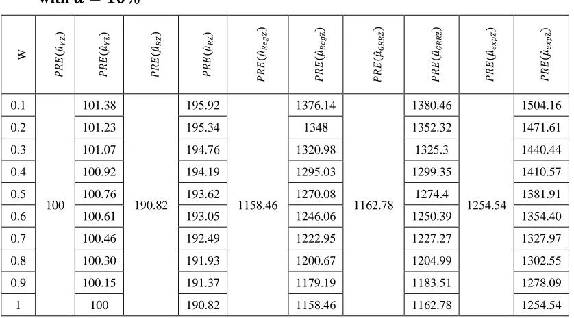
Table 5.1: Percent relative efficiencies of various estimators with respect to 𝝁̂𝒀𝒁. with 𝜶 = 𝟏𝟎%
W
𝑃
𝑅
𝐸
(𝜇
̂𝑌𝑍
)
𝑃
𝑅
𝐸
(𝜇
̂𝑌Ƶ
)
𝑃
𝑅
𝐸
(𝜇
̂𝑅𝑍
)
𝑃
𝑅
𝐸
(𝜇
̂𝑅Ƶ
)
𝑃
𝑅
𝐸
(𝜇
̂𝑅𝑒𝑔
𝑍
)
𝑃
𝑅
𝐸
(𝜇
̂𝑅𝑒𝑔
Ƶ
)
𝑃
𝑅
𝐸
(𝜇
̂𝐺𝑅
𝑅
𝑍
)
𝑃
𝑅
𝐸
(𝜇
̂𝐺𝑅𝑅
Ƶ
)
𝑃
𝑅
𝐸
(𝜇
̂𝑒𝑥𝑝𝑍
)
𝑃
𝑅
𝐸
(𝜇
̂𝑒𝑥𝑝
Ƶ
)
0.1
100
101.38
190.82
195.92
1158.46
1376.14
1162.78
1380.46
1254.54
1504.16
0.2 101.23 195.34 1348 1352.32 1471.61
0.3 101.07 194.76 1320.98 1325.3 1440.44
0.4 100.92 194.19 1295.03 1299.35 1410.57
0.5 100.76 193.62 1270.08 1274.4 1381.91
0.6 100.61 193.05 1246.06 1250.39 1354.40
0.7 100.46 192.49 1222.95 1227.27 1327.97
0.8 100.30 191.93 1200.67 1204.99 1302.55
0.9 100.15 191.37 1179.19 1183.51 1278.09
Table 5.2: Percent relative efficiencies of various estimators with respect to 𝝁̂𝒀𝒁 with 𝜶 = 𝟐𝟎% W 𝑃 𝑅𝐸 (𝜇 ̂𝑌𝑍 ) 𝑃 𝑅𝐸 (𝜇 ̂𝑌Ƶ ) 𝑃 𝑅𝐸 (𝜇 ̂𝑅𝑍 ) 𝑃 𝑅𝐸 (𝜇 ̂𝑅Ƶ ) 𝑃 𝑅𝐸 (𝜇 ̂𝑅𝑒𝑔 𝑍 ) 𝑃 𝑅𝐸 (𝜇 ̂𝑅𝑒𝑔 Ƶ ) 𝑃 𝑅𝐸 (𝜇 ̂𝐺𝑅 𝑅 𝑍 ) 𝑃 𝑅𝐸 (𝜇 ̂𝐺𝑅 𝑅 Ƶ ) 𝑃 𝑅𝐸 (𝜇 ̂𝑒𝑥𝑝𝑍 ) 𝑃 𝑅𝐸 (𝜇 ̂𝑒𝑥𝑝 Ƶ ) 0.1 100 105.51 183.56 203.03 793.04 1353.97 797.56 1358.49 845.18 1474.77
0.2 104.87 200.66 1255.32 1259.83 1361.84
0.3 104.24 198.35 1170.06 1174.58 1265.02
0.4 103.61 196.1 1095.65 1100.17 1181.08
0.5 102.99 193.89 1030.14 1034.65 1107.63
0.6 102.38 191.73 972.015 976.533 1042.8
0.7 101.77 189.62 920.103 924.62 985.171
0.8 101.17 187.56 873.454 877.972 933.6
0.9 100.58 185.54 831.308 835.825 887.179
1 100 183.56 793.041 797.558 845.175
Table 5.3: Percent relative efficiencies of various estimators with respect to 𝝁̂𝒀𝒁 with
𝜶 = 𝟑𝟎%
W 𝑃𝑅𝐸
(𝜇 ̂𝑌𝑍 ) 𝑃 𝑅𝐸 (𝜇 ̂𝑌Ƶ ) 𝑃 𝑅𝐸 (𝜇 ̂𝑅𝑍 ) 𝑃 𝑅𝐸 (𝜇 ̂𝑅Ƶ ) 𝑃 𝑅𝐸 (𝜇 ̂𝑅𝑒𝑔 𝑍 ) 𝑃 𝑅𝐸 (𝜇 ̂𝑅𝑒𝑔 Ƶ ) 𝑃 𝑅𝐸 (𝜇 ̂𝐺𝑅 𝑅 𝑍 ) 𝑃 𝑅𝐸 (𝜇 ̂𝐺𝑅 𝑅 Ƶ ) 𝑃 𝑅𝐸 (𝜇 ̂𝑒𝑥𝑝𝑍 ) 𝑃 𝑅𝐸 (𝜇 ̂𝑒𝑥𝑝 Ƶ ) 0.1 100 112.31 173.74 214.6 539.92 1322.31 544.76 1327.15 570.14 1433.22
0.2 110.79 209.13 1138.93 1143.77 1226.12
0.3 109.32 203.94 1000.22 1005.06 1071.45
0.4 107.88 199 891.624 896.469 951.549
0.5 106.48 194.29 804.301 809.147 855.872
0.6 105.12 189.8 732.558 737.403 777.753
0.7 103.79 185.51 672.565 677.41 712.764
0.8 102.5 181.42 621.654 626.499 657.852
0.9 101.23 177.49 577.909 582.754 610.841
1 100 173.74 539.92 544.76 570.14
Population II Source: Sousa et al. (2010)
𝑁 = 1000, 𝜌𝑦𝑥 = 0.8783, 𝑋̅ = 2, 𝑌̅ = 2, 𝑆𝑥 =2.4495, 𝑆𝑦 =1.4142 and 𝑛 =
Table 5.4: Percent relative efficiencies of various estimators with respect to 𝝁̂𝒀𝒁 with 𝜶 = 𝟏𝟎%
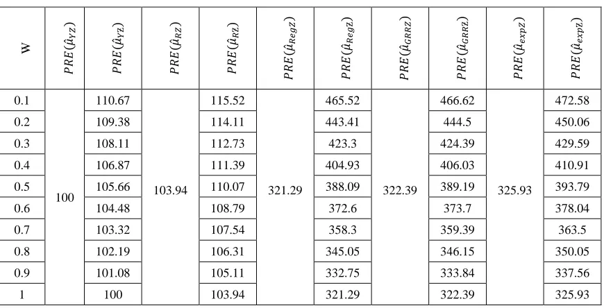
Table 5.5: Percent relative efficiencies of various estimators with respect to 𝝁̂𝒀𝒁 with
𝜶 = 𝟐𝟎% W 𝑃 𝑅𝐸 (𝜇 ̂𝑌𝑍 ) 𝑃 𝑅𝐸 (𝜇 ̂𝑌Ƶ ) 𝑃 𝑅𝐸 (𝜇 ̂𝑅𝑍 ) 𝑃 𝑅𝐸 (𝜇 ̂𝑅Ƶ ) 𝑃 𝑅𝐸 (𝜇 ̂𝑅𝑒𝑔 𝑍 ) 𝑃 𝑅𝐸 (𝜇 ̂𝑅𝑒𝑔 Ƶ ) 𝑃 𝑅𝐸 (𝜇 ̂𝐺𝑅 𝑅 𝑍 ) 𝑃 𝑅𝐸 (𝜇 ̂𝐺𝑅 𝑅 Ƶ ) 𝑃 𝑅𝐸 (𝜇 ̂𝑒𝑥𝑝𝑍 ) 𝑃 𝑅𝐸 (𝜇 ̂𝑒𝑥𝑝 Ƶ ) 0.1 100 102.69 104.3 107.23 398.31 444.75 399.32 445.76 404.26 451.55
0.2 102.39 106.9 439.07 440.07 445.76
0.3 102.08 106.57 433.52 434.53 440.11
0.4 101.78 106.24 428.12 429.12 434.6
0.5 101.48 105.91 422.84 423.85 429.23
0.6 101.18 105.58 417.7 418.71 424
0.7 100.88 105.26 412.68 413.68 418.88
0.8 100.59 104.94 407.78 408.78 413.89
0.9 100.29 104.62 402.99 404 409.02
1 100 104.3 398.31 399.32 404.26
W 𝑃 𝑅𝐸 (𝜇 ̂𝑌𝑍 ) 𝑃 𝑅𝐸 (𝜇 ̂𝑌Ƶ ) 𝑃 𝑅𝐸 (𝜇 ̂𝑅𝑍 ) 𝑃 𝑅𝐸 (𝜇 ̂𝑅Ƶ ) 𝑃 𝑅𝐸 (𝜇 ̂𝑅𝑒𝑔 𝑍 ) 𝑃 𝑅𝐸 (𝜇 ̂𝑅𝑒𝑔 Ƶ ) 𝑃 𝑅𝐸 (𝜇 ̂𝐺𝑅 𝑅 𝑍 ) 𝑃 𝑅𝐸 (𝜇 ̂𝐺𝑅 𝑅 Ƶ ) 𝑃 𝑅𝐸 (𝜇 ̂𝑒𝑥𝑝𝑍 ) 𝑃 𝑅 𝐸 (𝜇 ̂𝑒𝑥𝑝 Ƶ ) 0.1 100 110.67 103.94 115.52 321.29 465.52 322.39 466.62 325.93 472.58
0.2 109.38 114.11 443.41 444.5 450.06
0.3 108.11 112.73 423.3 424.39 429.59
0.4 106.87 111.39 404.93 406.03 410.91
0.5 105.66 110.07 388.09 389.19 393.79
0.6 104.48 108.79 372.6 373.7 378.04
0.7 103.32 107.54 358.3 359.39 363.5
0.8 102.19 106.31 345.05 346.15 350.05
0.9 101.08 105.11 332.75 333.84 337.56
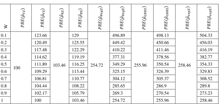
Table 5.6: Percent relative efficiencies of various estimators with respect to 𝝁̂𝒀𝒁 with 𝜶 = 𝟑𝟎%
W 𝑃𝑅𝐸
(𝜇
̂𝑌𝑍
)
𝑃
𝑅𝐸
(𝜇
̂𝑌Ƶ
)
𝑃
𝑅𝐸
(𝜇
̂𝑅𝑍
)
𝑃
𝑅𝐸
(𝜇
̂𝑅Ƶ
)
𝑃
𝑅𝐸
(𝜇
̂𝑅𝑒𝑔
𝑍
)
𝑃
𝑅𝐸
(𝜇
̂𝑅𝑒𝑔
Ƶ
)
𝑃
𝑅𝐸
(𝜇
̂𝐺𝑅
𝑅
𝑍
)
𝑃
𝑅𝐸
(𝜇
̂𝐺𝑅
𝑅
Ƶ
)
𝑃
𝑅𝐸
(𝜇
̂𝑒𝑥𝑝𝑍
)
𝑃
𝑅𝐸
(𝜇
̂𝑒𝑥𝑝
Ƶ
)
0.1
100
123.66
103.46 129
254.72
496.89
255.96
498.13
258.46
504.33
0.2 120.49 125.55 449.42 450.66 456.03
0.3 117.48 122.29 410.22 411.46 416.19
0.4 114.62 119.19 377.31 378.56 382.77
0.5 111.89 116.25 349.29 350.54 354.33
0.6 109.29 113.44 325.15 326.39 329.83
0.7 106.81 110.77 304.12 305.37 308.52
0.8 104.44 108.22 285.65 286.9 289.8
0.9 102.17 105.79 269.3 270.54 273.23
1 100 103.46 254.72 255.96 258.46
From the Table 5.1 to Table 5.6, we observe the following facts:
(i) The percent relative efficiencies of the all estimators with optional RRT decrease as the value of 𝑊 increases.
(ii) The proposed estimator 𝜇̂𝑒𝑥𝑝Ƶ is always more efficient than the various existing estimators considered in this paper.
(iii) It is important to note that various estimators with optional RRT model are always more efficient than the corresponding estimator with traditional RRT model.
(iv) The estimators with optional RRT are equally efficient to their corresponding estimators with traditional RRT model only when 𝑊 = 1. (see Remark: 2.1)
6. Conclusion: By applying optional RRT model in the estimator of Koyuncu et al (2014), we not only improve the efficiency of estimator suggested by Koyuncu et al (2014) but also obtain an estimator which is more efficient than Gupta et al (2014)’s estimators based on optional RRT model.
Acknowledgements: Authors are thankful to the editor and the two unknown learned referees for their useful and encouraging comments and suggestions, which led to the present improved version of the paper.
References
1. Bahl, S. and Tuteja, R.K. (1991). Ratio and product type exponential estimators. Information and Optimization Sciences, 12(1):159-163.
2. Cochran, W.G. (1977). Sampling Techniques. Third Edition, New Delhi, India: Wiley Eastern Limited
4. Gupta, S., Kalucha, G., Shabbir, J. and Dass, B.K. (2014). Estimation of finite population mean using Optional RRT Models in the presence of non sensitive auxiliary information. American journal of Mathematical and Management Sciences, 33:147-159.
5. Gupta, S., Mehta, S., Shabbir, J. and Dass, B.K. (2013). Generalized scrambling in quantitative optional randomized response models. Communications in Statistics- Theory and Methods. 42(20):1-9.
6. Gupta, S., Shabbir, J. and Sehra, S. (2010). Mean and sensitivity estimation in optional randomized response models. Journal of Statistical and Planning Inference. 140(10):2870-2874.
7. Gupta, S., Shabbir, J., Sousa, R. and Corte-Real, P. (2012). Estimation of the mean of a sensitive variable in the presence of auxiliary information. Communication in Statistics- Theory and Methods. 41:2394-2404.
8. Huang, K.C. (2010). Unbiased estimators of mean, variance and sensitivity level for quantitative characterstics in finite population sampling. Metrika. 71:341-352. 9. Kalucha, G., Gupta, S. and Dass, B.K. (2015). Ratio estimation of finite
population mean using optional randomized response models. Journal of Statistical Theory and Practice. 9:633-645.
10. Koyuncu, N., Gupta, S. and Sousa, R. (2014). Exponential-type estimators of the mean of a sensitive variable in the presence of non sensitive auxiliary information. Communications in statistics- Simulation and Computation, 43: 1583-1594.
11. Singh, H.P. and Solanki, R.S. (2012). Improved estimation of population mean in simple random sampling using information on auxiliary attribute. Applied Mathematics and Computation. 218:7798-7812.
12. Singh, H.P. and Tarray, T.A. (2014). A stratified Mangat and Singh’s optional randomized response model using proportional and optimal allocation. Statistica, anno. 74(1):65-83.
13. Sousa, R., Shabbir, J., Corte-Real, P., and Gupta, S., (2010). Ratio estimation of the mean of a sensitive variable in the presence of auxiliary information. Journal of Statistical Theory and Practice. 4(3):495-507.
14. Tarray, T.A., Singh, H.P. and Zaizai, Y. (2015). A dexterous optional randomized response model. Sociological Methods and Research. 46(3): 565-585.