https://doi.org/10.5194/tc-12-1103-2018
© Author(s) 2018. This work is distributed under the Creative Commons Attribution 4.0 License.
Atmospheric influences on the anomalous 2016
Antarctic sea ice decay
Elisabeth Schlosser1,2, F. Alexander Haumann3,4, and Marilyn N. Raphael5
1Institute of Atmospheric and Cryospheric Sciences, University of Innsbruck, Innsbruck, Austria 2Austrian Polar Research Institute, Vienna, Austria
3Environmental Physics, Institute of Biogeochemistry and Pollutant Dynamics, ETH Zürich, Zurich, Switzerland 4British Antarctic Survey, Cambridge, UK
5Department of Geography, University of California, Los Angeles, California, USA
Correspondence:Elisabeth Schlosser (elisabeth.schlosser@uibk.ac.at) Received: 2 September 2017 – Discussion started: 22 September 2017
Revised: 6 January 2018 – Accepted: 26 February 2018 – Published: 28 March 2018
Abstract.In contrast to the Arctic, where total sea ice extent (SIE) has been decreasing for the last three decades, Antarc-tic SIE has shown a small, but significant, increase during the same time period. However, in 2016, an unusually early onset of the melt season was observed; the maximum Antarc-tic SIE was already reached as early as August rather than the end of September, and was followed by a rapid decrease. The decay was particularly strong in November, when Antarctic SIE exhibited a negative anomaly (compared to the 1979– 2015 average) of approximately 2 million km2. ECMWF In-terim reanalysis data showed that the early onset of the melt and the rapid decrease in sea ice area (SIA) and SIE were associated with atmospheric flow patterns related to a posi-tive zonal wave number three (ZW3) index, i.e., synoptic sit-uations leading to strong meridional flow and anomalously strong southward heat advection in the regions of strongest sea ice decline. A persistently positive ZW3 index from May to August suggests that SIE decrease was preconditioned by SIA decrease. In particular, in the first third of Novem-ber northerly flow conditions in the Weddell Sea and the Western Pacific triggered accelerated sea ice decay, which was continued in the following weeks due to positive feed-back effects, leading to the unusually low November SIE. In 2016, the monthly mean Southern Annular Mode (SAM) index reached its second lowest November value since the beginning of the satellite observations. A better spatial and temporal coverage of reliable ice thickness data is needed to assess the change in ice mass rather than ice area.
1 Introduction and previous work
Sea ice plays a critically important role in the cryosphere as well as the global climate system. It modifies heat and mass exchange processes. Sea ice has a very high albedo com-pared to open water; thus when present, it greatly increases the surface reflectivity. It also reduces the exchange of heat and moisture between the ocean and the lower atmosphere. Strong positive feedback effects related to sea ice changes have consequences for both atmosphere and ocean. Melting of sea ice rapidly decreases the surface albedo and increases turbulent heat exchange between ocean and atmosphere; it thus strongly influences the surface energy balance of the ocean (e.g., Stammerjohn et al., 2012), which in turn affects sea ice itself. Formation and melt of sea ice also influences the seawater salinity by releasing salt (brine rejection) upon freezing and freshwater upon melting. These fluxes dominate the surface freshwater flux balance of the seasonally sea-ice-covered Southern Ocean and thereby strongly influence the ocean overturning circulation (Haumann et al., 2016), which is critical for exchanging heat and carbon between the deep ocean and the atmosphere. Therefore, Antarctic sea ice plays an active role in the global climate system.
early onset of the seasonal ice melt was observed. The max-imum Antarctic SIE was reached a month earlier, in August, rather than the end of September, and was followed by rapid decrease until the summer when record minimum SIE was observed. The sea ice area (SIA), the total area actually cov-ered by ice, started to exhibit values below the long-term av-erage as early as July, with only a brief return to normal in late August when the general sea ice retreat began. The de-cay was particularly strong in November, when Antarctic SIE exhibited a negative anomaly (compared to the 1979–2015 average) of 1.84 million km2, which is unprecedented in the satellite era (since 1979) and, combined with reduced Arc-tic sea ice, led to a distinct minimum in global SIE (NSIDC, 2016).
The present study is motivated by this unusual behavior of Antarctic sea ice in 2016. Sea ice retreat is influenced by atmospheric as well as oceanic processes. Local atmospheric influences on sea ice, both dynamic and thermodynamic, act on a relatively short timescale with an immediate response of the sea ice. In this study, we solely focus on the local at-mospheric influences on sea ice retreat and discuss related possible reasons for the observed anomalous sea ice decay.
Locally, changes in SIE and SIA can be caused by melt-ing or freezmelt-ing and by sea ice dynamics that influence ice advection, ice divergence, and convergence (e.g., Enomoto and Ohmura, 1990). On a short timescale (days to weeks), both processes are strongly dependent on atmospheric influ-ences, i.e., thermodynamics of the ocean–atmosphere inter-face and wind stress on the floating ice (e.g., Watkins and Simmonds, 2000). Oceanic influences mainly play a role on longer timescales, such as seasonal and interannual varia-tions (e.g., Gordon and Huber, 1990; Martinson, 1990). In particular, while changes in the timing of sea ice retreat seem to have a strong influence on the timing of the following ad-vance, advance and subsequent retreat are only weakly re-lated (Stammerjohn et al., 2012). This relation suggests a strong oceanic thermal feedback that accelerates or deceler-ates fall freeze onset (Stammerjohn et al., 2012). In a recent study, Su (2017) stated that the location of the sea ice edge at the SIE maximum is strongly correlated with the upper-ocean stratification in early winter (April–June), consistent with the findings by Lecomte et al. (2017). The seasonal influence of the ocean on SIE has been the subject of a number of stud-ies. Hall and Visbeck (2002) show that the strength and po-sition of the westerlies influence northward Ekman transport and therefore the SIE as well as upwelling of warmer water closer to the continent. This effect can cause stronger retreat of sea ice in summer, when the ice edge is farther south, and expansion of sea ice in winter (e.g., Lee et al., 2017).
Enomoto and Ohmura (1990) investigated the relationship of the sea ice edge advance and retreat and the semi-annual oscillation of the circumpolar trough. The ice drift depends on the position of the sea ice edge relative to the Antarc-tic convergence line (Enomoto and Ohmura, 1990), which moves according to the semi-annual oscillation of the
cir-cumpolar trough (Meehl, 1991). This leads to ice divergence when the ice edge is north of the convergence and trans-port of ice towards the coast when the ice edge is south of the Antarctic convergence line. The velocity of the ice drift amounts to 1–2 % of the surface wind speed, when the direc-tion of the ice drift is turned by 10–40◦to the left of the di-rection of the atmospheric flow, an average value of approxi-mately 30◦was found (Kottmeier et al., 1992; Kottmeier and Sellmann, 1996; Nansen, 1902). Therefore, the meridional ice transport that affects the latitudinal extent of the sea ice is primarily driven by meridional winds, but zonal winds can also have an influence, particularly in the Ross and Weddell seas where the sea ice edge extends to lower latitudes into the westerly wind belt during winter (Haumann, 2011). Hol-land and Kwok (2012) investigated the influence of surface winds on Antarctic sea ice changes over the period 1992 to 2010. They state that while in most parts of West Antarctica mainly wind-driven changes in ice advection are responsible for the observed sea ice concentration (SIC) trends, wind-driven thermodynamic changes dominate in all other parts of the Southern Ocean. Haumann et al. (2014) and Kwok et al. (2017) show that meridional wind changes also play a major role in driving the sea ice trends over the entire satel-lite record. In some regions, zonal winds are also important for zonal redistribution of the ice (Haumann, 2011; Kwok et al., 2017). This means that changes in both the meridional and zonal components of the atmospheric circulation can in-duce sea ice anomalies, either through associated tempera-ture anomalies or through ice transport anomalies.
modeling studies suggest a strong influence of interannual and decadal tropical variability, especially in the Pacific, on Antarctic sea ice anomalies through the atmospheric circula-tion (Meehl et al., 2016; Purich et al., 2016; Schneider and Deser, 2017) and oceanic feedbacks (Stuecker et al., 2017).
In the past 37 years covered by satellite data, variations in the total Antarctic SIE have been small since large contrast-ing regional variations, both positive and negative deviations from the mean, cancel each other. Large regional anomalies in SIC can be caused by stable synoptic situations, where at-mospheric flow conditions that persist over several days or are dominant over several weeks lead to a southward (north-ward) ice transport combined with warm (cold) air advection (e.g., Massom et al., 2006; Schlosser et al., 2011). Turner et al. (2009) stated that the long-term increase in Antarctic SIE is mostly caused by an increase in the Ross Sea sector, which is strongly influenced by the strength and position of the Amundsen Sea Low (ASL) (Raphael et al., 2015). Turner et al. (2009) also related stratospheric ozone loss to the ob-served increase in Antarctic SIE and found that the strength-ening of the westerlies, which is related to ozone depletion, deepens the ASL. They conclude, however, that the observed SIE increase might still be within the limits of natural vari-ability. Haumann et al. (2014) found that, on multidecadal timescales, changes in Antarctic SIE are linked to changes in the strength of meridional winds that are caused by a zon-ally asymmetric decrease in high-latitude surface pressure, the latter possibly being related to stratospheric ozone deple-tion, greenhouse gas increase, or natural variability. While increased southerly (and potentially westerly) winds most likely fueled the long-term increase of Antarctic sea ice over the satellite era, we here hypothesize that increased northerly winds and an associated warm air advection triggered the negative Antarctic sea ice anomaly in 2016.
Two recent studies investigated the observed unusually fast retreat in the spring of 2016. Turner et al. (2017), after a discussion of the climatological mean behavior of Antarc-tic sea ice, consider the spatial differences of SIE anomalies and their temporal changes for five different sectors of the Southern Ocean. While in the Weddell Sea a marked change from positive to negative SIE anomalies occurred in Novem-ber, the Amundsen–Bellingshausen seas (ABS) and the In-dian Ocean showed mainly negative anomalies throughout the melt season. The Ross Sea and West Pacific sectors exhibited both positive and negative SIE anomalies during the entire period. They argue that the decrease of SIE at a record rate is linked to record surface pressure anomalies, mainly in the Weddell Sea and Ross Sea sectors of Antarc-tica, and the related meridional flow and corresponding warm air advection (Turner et al., 2017). Alternatively, Stuecker et al. (2017) hypothesize that the anomalously low SIE in November–December 2016 was largely related to positive sea surface temperature anomalies due to the extreme El Niño event peaking in December–February 2015–2016 that
persisted throughout the winter and the concurrent negative phase of the SAM.
Generally, changes in both oceanic and atmospheric pro-cesses could have been responsible for the observed 2016 anomaly. In the present study we investigated in detail the onset and temporal evolution of the sea ice retreat (consider-ing both SIA and SIE, as well as SIC) and the contributions of various parts of the Southern Ocean. A detailed analysis of the evolution of the SIA and SIE deficits shows a rapid growth of regional anomalies, suggesting an atmospheric ori-gin of these changes. We compared those changes to ice drift data and related it to the general atmospheric flow condi-tions derived from the European Centre for Medium-Range Weather Forecasts (ECMWF) reanalysis data and considered the relationship to SAM and ZW3 indices and patterns.
2 Data and methods 2.1 Sea ice data
Sea ice data are provided by the National Snow and Ice Data Center (NSIDC). SIC is derived from Nimbus-7 SMMR and DMSP SSM/I-SSMIS passive microwave data (Maslanik and Stroeve, 1999). The data set is generated from brightness temperature and designed to provide a consistent time series of SIC. The data are provided in polar stereographic projec-tion at a grid cell size of 25 km×25 km. We use the Cli-mate Data Record version 2 NASA Team algorithm (CDR NT; Meier et al., 2013) data for the period 1979 to 2015 as a baseline climatological record. These data are com-pared to the near-real-time data (NRT; http://nsidc.org/data/ NSIDC-0081, last access: 23 March 2018; Maslanik and Stroeve, 1999) from January 2015 to June 2017, which are also derived from passive microwave data using the NASA Team algorithm. Days with a large number of missing pixels in the SIC have been removed from the NRT data. The result-ing SIE anomalies for the overlappresult-ing year 2015 agree well (Fig. 1). To create monthly mean ice drift fields, the low-resolution sea ice drift product of the EUMETSAT Ocean and Sea Ice Satellite Application Facility (OSI SAF, available at www.osi-saf.org, last access: 23 March 2018; Lavergne et al., 2010) was used.
Figure 1.Monthly mean SIE anomalies since 1979 with respect to the 1979 to 2015 climatology. The period 1979 through 2015 is derived from the CDR NT data (green; Meier et al., 2013; provided by NSIDC). The period January 2015 through June 2017 is derived from the NRT data (red; Maslanik and Stroeve, 1999, updated daily; provided by NSIDC). Green shading shows the±2 standard deviation of the CDR NT record and the green dashed line shows the respective long-term trend derived from linear regression analysis. The red dashed line shows the long-term trend for the period 1979 through June 2017 when extending the CDR NT record using the period January 2016 through June 2017 from the NRT record.
2.2 ECMWF reanalysis data
ECMWF Interim reanalysis (ERA-Interim) data were em-ployed to investigate atmospheric flow conditions. The re-analysis data are available from 1979 to present. The hor-izontal resolution is T255, corresponding to approximately 79 km. The model has 60 vertical levels, with the highest level at 0.1 hPa. A detailed description of ERA-Interim is given in Dee et al. (2011). We used monthly mean sea level pressure and vertically integrated northward heat flux, de-rived from the daily mean values. The reanalysis data were used for investigation of ZW3 patterns and analysis of sur-face pressure fields and cyclone activity.
2.3 SAM and ZW3 indices
Meridional transport of heat and moisture in the high lati-tudes of the Southern Hemisphere is carried out by the asym-metric component of the circulation also known as quasi-stationary waves (Raphael, 2004). Together, ZW1 and ZW3 represent the largest proportion of this asymmetry (van Loon and Jenne, 1972). The asymmetry described by these zonal waves is revealed when the zonal mean is subtracted from the geopotential height field and coherent pattern of zonal anomalies and their associated flow become apparent. Both ZW1 and ZW3 have preferred regions of meridional flow, guiding the meridional transport of heat and moisture into and out of the Antarctic. ZW1 and ZW3 vary with each other so that when ZW3 is strong, ZW1 is weak and vice versa. An index of ZW3 based on its amplitude defined by Raphael (2004) shows that ZW3 has positive and negative phases, where a positive phase indicates strong meridional flow and a negative phase more zonal flow. A climatology of this index shows that ZW3 tends to be negative from September through December, a period of time when ZW1
is dominant in the field (Raphael, 2004). Since it exerts con-trol on the meridional flow, ZW3 influences the variability of Antarctic sea ice dynamically and thermodynamically as illustrated in Raphael (2007).
3 Results
3.1 Temporal evolution of Antarctic sea ice extent and area
In Fig. 1 monthly SIE anomalies from January 1979 to June 2017 are displayed. Until 2015, only relatively small varia-tions and a generally positive trend can be seen. This trend is abruptly interrupted in November 2016, when monthly mean SIE was almost 2 million km2 lower than in the preceding year. This value is clearly outstanding: the negative deviation from the mean reaches almost 4 times the standard deviation (2.06 million km2) of the 1979 to 2015 period. Trends are calculated from the CDR data until the end of 2015 and for the period including the most recent 17 months from NRT data, respectively. The extension of the period by these latter 17 months reduces the positive trend from 0.24 million km2 per decade (1979–2015) to 0.16 million km2per decade.
Figure 2 shows the daily Antarctic SIE (Fig. 2a) and SIA (Fig. 2b) for the year 2016 together with the 1979–2015 average. The gray shading refers to the 2 standard devi-ations (1979–2015). While, on average, SIE increases un-til the end of September, in 2016 a sudden decrease oc-curred in the last third of August. After the first week of September SIE fell below the long-term average and never recovered during the rest of the year. The monthly mean anomaly in SIE increased from −0.1 million km2 in Au-gust to a maximum deviation from the monthly mean of −1.84 million km2in November. In December the anomaly amounted to−2.33 million km2. The SIA exhibited negative deviations from the mean already in June and July, briefly reached values close to the average again at the end of August and thereafter remained below the average for the rest of the year. The monthly mean SIA anomalies for November and December 2016 are −1.98 million and−1.55 million km2, respectively, and generally preceded the SIE anomalies. The SIE deficit (shaded pink vs. dashed gray, 2 standard devi-ations; 1979–2015) also suggests that there were two dis-tinct periods of decline: the first one in late August to mid-September and the second one in the first half of November. While the first period saw a corresponding decline in SIA, the second period is not as distinct for SIA. The overall largest SIA deficit of 2.24 million km2 occurred on 18 November, whereas the largest SIE deficit of 2.8 million km2was seen approximately 1 month later, on 14 December. The sea ice never did recover in austral summer 2016–2017; in February 2017 the monthly mean SIE amounted to 2.27 million km2, which is the lowest February value since beginning of the satellite measurements in 1979. However, the monthly mean SIA was, with 1.63 million km2, only the second lowest one; here the absolute minimum occurred in February 1993 (1.4 million km2).
In Fig. 2c the SIA change (daily temporal derivative of the SIA) is shown. Again, the red and black lines refer to 2016 and the climatological mean (1979–2015), respectively.
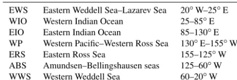
Table 1.Regions used for the regional analysis (Fig. 5).
EWS Eastern Weddell Sea–Lazarev Sea 20◦W–25◦E WIO Western Indian Ocean 25–85◦E EIO Eastern Indian Ocean 85–130◦E WP Western Pacific–Western Ross Sea 130◦E–155◦W ERS Eastern Ross Sea 155–125◦W ABS Amundsen–Bellingshausen seas 125–60◦W WWS Western Weddell Sea 60–20◦W
The SIA change can be interpreted as ice melt or compaction when it is negative and as new ice formation when it is pos-itive. The pink shading indicates anomalously high melt or low freezing periods, and the blue shading the opposite. A first, a very short period with SIA decrease was observed as early as in mid-July when the SIA change reached negative values for the first time.
It can be clearly seen that, until August, periods with grow-ing and shrinkgrow-ing SIA deficit alternate, whereas from the end of August on almost only negative deviations from the mean are found, with negative SIA changes for the rest of the year. In addition to the periods mentioned above, a further period with strong sea ice decline can be seen in mid-October. 3.2 Regional sea ice changes
3.2.1 SIC anomalies and corresponding influence of cyclonic activity
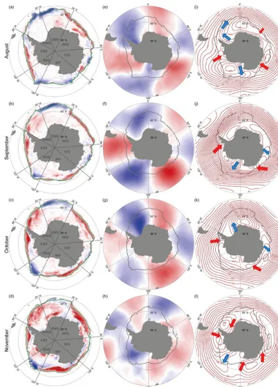
To investigate which areas contributed predominantly to the observed changes, Antarctica was divided into seven sub-areas (see Table 1), the definition following specifically the regional SIC anomalies displayed in Fig. 3a–d for the months August to November 2016. This division is finer than the five sub-areas used in previous studies (e.g., Turner et al., 2017) and thus allows a detailed discussion of the temporal and spa-tial development of the sea ice retreat. In particular, the sub-division of the Weddell Sea was necessary due to the differ-ent behavior of the western and eastern part. The SIC anoma-lies, as usual, exhibit strong regional differences, with areas with positive deviations alternating with areas of negative deviations. In August, the total SIE is only 0.1 million km2 smaller than the long-term average (1979–2015). The contri-butions of areas with negative SIC anomalies mostly counter-act those of areas with positive anomalies. Largest negative SIC anomalies are found at the eastern edge of the Eastern Weddell Sea (EWS) and in the Western Indian Ocean (WIO), where also the sea ice edge (gray contour line in Fig. 3a) is already distinctly farther south than on average (green con-tour line). In the Eastern Indian Ocean (EIO), only a very small area, centered at approximately 125◦E, shows nega-tive anomalies of SIC; otherwise SIC anomalies are slightly positive. In the western Pacific/western Ross Sea (WP), the sea ice edge is also close to the long-term average; positive deviations in SIC are found near 150◦E and at the northern
edge of the Ross Sea. The ABS show southward deviations from the mean sea ice edge, whereas both the Western Wed-dell Sea (WWS) and EWS exhibit positive SIC anomalies between approximately 35◦W and 0◦, associated with a sea ice edge farther north than on average.
Generally, SIC depends on ice dynamics (advection) and thermodynamics, both, on short timescales, being strongly influenced by the atmospheric flow. Surface winds above the Southern Ocean depend mostly on the cyclone activity in the circumpolar trough (Simmonds et al., 2003). Figure 3i–l show the monthly mean surface pressure for the correspond-ing months. Arrows indicate the approximate main surface flow direction related to changes in SIC or sea ice edge. In the Southern Hemisphere, the air circulates clockwise around the center of a cyclone, meaning a northerly (southerly) flow at the western (eastern) flank of the cyclone. Northerly flow leads to compaction of the ice and/or advection of warmer air and thus a southward displacement of the sea ice edge by compaction and/or melt. In contrast, a southerly flow is related to northward drift of the ice and formation of new ice close to the coast due to cold air advection from the continent over leads and polynyas that develop as the ice is pushed away. The strong westerly flow at the northern edge of the cyclone can, via Ekman transport (e.g., Hall and Vis-beck, 2002), also lead to net northward transport of sea ice and thus a northward displacement of the sea ice edge. In Fig. 3e–h the vertically integrated northward heat flux from ERA-Interim is displayed. Positive (negative) values sug-gest northward transport of cold (warm) air, which in most cases in Antarctica means cold (warm) air advection. Strictly speaking, since advection is proportional to the meridional temperature gradient, the heat flux alone does not necessar-ily prove warm air advection. However, the spatial temper-ature distribution around Antarctica is basically zonal, and thus a northerly (southerly) flow is practically always associ-ated with warm (cold) air advection. It has also been shown in Antarctic precipitation studies (e.g., Gorodetskaya et al., 2014) that considerable warm air (and thus moisture) advec-tion in the circumpolar trough is usually observed in a thick layer from the surface to the upper troposphere, which in-fluences not only the sensible heat flux at but also longwave radiation to the surface, both favoring sea ice melt. A strong signal in the vertically integrated meridional heat flux thus supports our findings. The air mass transport agrees very well with the general flow direction derived from the surface pres-sure field (see Fig. 3i–l and arrows herein).
anomaly (Fig. 3e). The area is rather restricted due to the con-fluent flow. In the EWS and the WIO, there was a weak, but extended, low pressure system that caused a weak northerly flow and warm air advection towards the western edge of the WIO associated with the negative SIC anomalies. However, most of the WIO was under the influence of a very weak pressure gradient, and consequently no distinct flow condi-tions prevailed.
In September (Fig. 3b), positive SIC anomalies occurred in the EWS, EIO, and ERS. The area with negative anoma-lies around 125◦E extended eastward across the entire WP. Additionally, SIC anomalies in the ABS and WWS were largely negative. The low pressure system in the Pacific Ocean (Fig. 3j) intensified and moved eastwards, extended across the Ross and Bellingshausen seas, which resulted in positive (negative) SIC anomalies at its western (eastern) flank. The WP was still influenced by the warm air advec-tion on the low centered in the EIO. The positive anomalies in the EIO are associated with an area of cold air advection (Fig. 3f and j). The negative SIC anomalies between 180◦W and approximately 160◦W (WP) are unexpected since this area is influenced by the ASL. In the northern parts of the EWS, positive SIC anomalies are observed, possibly related to the strong westerly flow resulting in zonal and meridional ice advection (Fig. 6b) due to a northeastward Ekman trans-port.
In October (Fig. 3c), the SIC anomalies occurred in the same areas as in September but were more strongly devel-oped. The ASL stretched eastward (Fig. 3k) and extends now across the ABS. In the EWS, a strong low pressure system has developed, leading to a northerly flow and warm air ad-vection in the WIO, where strong negative SIC anomalies are observed. The Eastern Indian Ocean/western Pacific low extended northwards, although with a weaker pressure gradi-ent. SIE in the EIO (Fig. 5g) changed very little and slightly less negative SIC anomalies occurred. The negative anomaly in SIE of the WIO (Fig. 5d) remained nearly constant in September and October.
In November, the WIO exhibited strong negative anoma-lies in SIC (Fig. 3d) and SIE (Fig. 5d), which contributed to the pronounced melt period in the first half of Novem-ber (Fig. 2c). Also, large negative deviations from the mean SIC (Fig. 3d) occurred in the WP, the ABS, and the WWS, whereas positive deviations in SIC were found around the sea ice edge in the EWS, and the ERS. In the southeastern Weddell Sea (Fig. 3d), negative SIC anomalies prevail, and the opening of the Weddell Sea polynya over Maud Rise (see also Sect. 3.2.3), which reoccurred more strongly in 2017 (not shown), becomes apparent.
Since we are considering monthly means here, a signal that is still visible in a monthly mean has to have been predom-inant over the majority of days during that month or has to have been very strong over a shorter time period. The lat-ter was the case at the end of August and also in Novem-ber: in the first third of the month the prevailing northerly
flow with warm air advection was very strong and thus cru-cial for triggering the increased melt. This situation is shown in Fig. 4, where the meridional heat flux (Fig. 4a) and the mean sea level pressure (Fig. 4b) for 1–10 November 2016 is displayed. It suggests that the strongest contribution to the monthly mean meridional heat flux (Fig. 3h) stems from the first third of the month. Figure 4b shows the corresponding surface pressure.
Between an extended low pressure system above the East-ern Indian Ocean/westEast-ern Pacific and a high pressure ridge in the Ross Sea, a strong northerly flow with warm air advection induced large negative SIC anomalies in that area. Similarly, in the western and central Weddell Sea, a northeasterly flow at the eastern flank of a low pressure system is associated with strong negative SIC anomalies. In the WIO, the picture is not as straightforward; oceanic memory effects may play a role here.
3.2.2 Temporal evolution of regional SIE and SIA To get a deeper insight into the spatial origin of the anoma-lies in SIE and SIA, in Fig. 5 the daily values of SIE, SIA, and SIA changes are displayed (similar to Fig. 2, for details see figure caption) for the different regions shown in Fig. 3. The EIO and ERS regions did not contribute to the acceler-ated sea ice decay. They have predominantly positive anoma-lies in SIE, SIA, and SIC. The EWS, WP, and WWS regions contributed to the negative SIE and SIA anomalies through strong events associated with the corresponding atmospheric flow discussed above, whereas the WIO and ABS exhibited more or less continuous negative deviations from the long-term mean. These developments are most clearly seen in the respective deficits of SIE and SIA shown at the bottom of the Fig. 5 plots. In the EWS, both SIA and SIE stayed above the long-term average, but contributed strongly to the negative anomaly through a distinct event evolving in November.
Figure 4.Mean vertically integrated meridional heat fluxes (positive northward)(a)and sea level pressure(b)from ERA-Interim (Dee et al., 2011) for the period 1–10 November 2016. The gray contour line denotes the mean sea ice edge (15 % SIC).
3.2.3 Ice drift
Ice drift influences SIE, SIA, and SIC in various ways. For example, northerly winds close to the ice edge lead to a southward sea ice compaction when the SIC is well below 100 % and to ridging and rafting, i.e., ice thickening, when the SIC is close to 100 %. Southerly winds close to the coast imply offshore transports that can cause coastal polynyas. These polynyas are usually quickly closed by new ice forma-tion due to associated cold air advecforma-tion from the continent. Strong westerly winds can lead to an eastward redistribution of the ice with a northerly component due to Ekman trans-port. Apart from that, convergence and confluence, as well as divergence and diffluence, in the main atmospheric flow can locally change SIC.
Since sea ice drift is strongly influenced by surface winds and might have contributed to the 2016 SIC anomalies, we examine the monthly mean ice motion from August to November 2016, illustrated in Fig. 6. It shows generally good agreement with the sea level pressure fields shown in Fig. 3, taking into consideration the corresponding wind fields dis-cussed in Sect. 3.2.1. Only in areas where SIE is already small, i.e., in the EIO and the eastern half of the ABS in Oc-tober and November, does the correlation between ice drift and wind direction more or less disappear due to the low res-olution of the plotted ice drift. In August, the large low pres-sure system above the Weddell and Lazarev seas is associated with clockwise ice drift in the Weddell Sea and drift towards the continent at its eastern flank. With an increasing pres-sure gradient in September, the drift increases at the northern flank, whereas the southward drift at its eastern flank disap-pears due to a predominantly westerly flow in the Lazarev
Sea. The ice drift connected to the ASL is best developed in September, with strong southerly (northwesterly) flow at the western (eastern) flank of the cyclone, contributing to the positive SIC anomaly in the ERS (Fig. 3b).
Figure 6.Monthly mean sea ice drift (arrows) for the months August to November 2016(a–d)derived from the low-resolution sea ice drift product of OSI SAF (www.osi-saf.org; Lavergne, et al., 2010). White shading shows the respective monthly mean SIC derived from the NRT data (red; Maslanik and Stroeve, 1999, updated daily; provided by NSIDC). The gray contour line shows the 15 % SIC line.
3.3 General atmospheric flow conditions during the melt season 2016
After having investigated in Sect. 3.2.1 the local meridional atmospheric flow related to sea ice changes specifically for individual low pressure systems (cyclones) observed during the melt period, we now want to consider the large-scale gen-eral atmospheric flow conditions.
3.3.1 ZW3
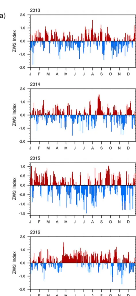
The monthly mean sea level pressure and meridional heat advection shown in Fig. 3 have a clear signal of ZW3, most strongly in August and October. Given these patterns, we ex-amine the ZW3 index for the period of ice decay. Figure 7a shows the daily ZW3 index for 2013–2016. The years 2013– 2015 are shown to put 2016 into perspective. Clearly, 2016 shows a distinctly different picture from the preceding years 2013–2015. While in 2013–2015 the ZW3 index alternated between positive and negative values throughout the year, in
2016 the ZW3 index was almost continuously positive over a longer time period. The largest differences occur in the cold season, namely mid-April to June, and, with short interrup-tions, well into August. In 2016, the positive ZW3 index is predominant from mid-April far into July and, with short in-terruptions, until mid-October. The sudden and unexpected decrease in SIE at the end of August comes after a prolonged period of positive ZW3 indices, whereas in November, when the record minimum SIE was observed, the ZW3 index is highly variable, both positive and negative. Given the influ-ence of ZW3 on the sign and strength of the sensible heat flux between atmosphere and ocean and thus on sea ice growth or melt (Raphael, 2007), we suggest that the persistent presence of a positive ZW3 index in the winter months preconditioned the ice for melt.
Figure 7.
500 hPa geopotential height field in November 2016, thus elucidating the asymmetry in the circulation suggested by the index. In August, as expected from the sign of the ZW3 in-dex and the mean sea level pressure distribution in Fig. 6a, a distinct ZW3 pattern can be seen, leading to fairly strong meridional flow and thus meridional heat exchange in the respective areas described in Sect. 3.2.1. While in Septem-ber the pattern is disturbed in the Atlantic sector (no distinct meridional flow, see Fig. 4b), in October it reappeared, but was no longer as well-defined as in August. In November,
while no clear ZW3 pattern is found, a distinct meridional flow can be seen around the Ross Sea and in the Weddell Sea in the first third of the month (see Fig. 4e). A clear ZW3 pat-tern is not expected here since the amplitude of the wave as shown in Fig. 7a is negative for most of the month. However, while a positive ZW3 index is not coincident with the de-crease in November, its persistence in the preceding months will have preconditioned the ice so that the effect of any other activity that promotes ice loss would be amplified. The flow pattern associated with the strong negative anomaly in the 500 hPa geopotential height above the Weddell Sea is con-sistent with the strong melt there due to warm air advection from the north.
Figure 8 illustrates the 2016 anomaly in the meridional heat flux for the entire year 2016 (Fig. 8a) as well as the period August to November 2016 only (Fig. 8b) with respect to the climatological mean of the period 1979–2015. Both the positive and the negative anomalies are stronger developed in the latter period, which agrees well with the prevailing ZW3 pattern described above.
3.3.2 Southern Annular Mode
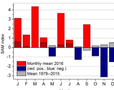
Figure 9 shows the monthly mean SAM index based on the calculation of Marshall (2003) for 2016 and the climatolog-ical monthly means calculated for the period 1979–2015. In November, the month with the largest ice loss, the SAM in-dex is highly negative; in fact, it is the second lowest SAM index since the start of the satellite sea ice observations. This low SAM index would suggest a rather meridional flow, re-sulting in a comparatively large meridional exchange of heat. Differing from ZW3, which has been strongly positive al-ready from May on and continuing during the entire winter months, thus hinting at increased meridional flow, the SAM index is positive in most months. However, as mentioned above, it should be kept in mind that SAM explains only part of the variability of the circulation, and large regional differ-ences in the flow pattern can occur. Additionally, the monthly means are not always meaningful since periods with positive and negative indices can cancel each other.
4 Discussion and conclusion
Figure 7. (a)Daily ZW3 index 2013–2016 (see Sect. 2.3 for details).(b)Monthly 500 hPa geopotential height zonal mean anomalies from ERA-Interim (Dee et al., 2011) for the period August–November 2016. Hatched areas indicate strongly negative values.
Figure 9.Monthly mean SAM index for 2016 and climatological monthly mean SAM index 1979–2015 (after Marshall, 2003).
discussed by Clem et al. (2017). The influence of ZW3 is reduced in November, whereas the phase of the SAM was strongly negative, its index reaching an almost record neg-ative value. The first third of November was under the in-fluence of strong warm air advection in the areas with neg-ative sea ice anomalies. This relneg-atively short, but intense, period triggered the accelerated ice melt, which was being continued in the following weeks due to the positive feed-back effects of the ice melt, i.e., lower albedo of the open vs. ice-covered ocean and increased turbulent heat flux from the ocean. The timing of this triggering was crucial for the increased melt; it happened exactly at the height of the melt season when conditions were set for melt anyway (strong ra-diation, high air temperatures).
Our results agree well with the general findings of Turner et al. (2017). While they stress the comparison of conditions in 2016 with the climatological means of amount and tim-ing of SIE minima and maxima as well as mean location and intensity of cyclones, our study looks more closely at both the temporal and spatial evolution of SIA, SIE, and the de-velopment of the anomalies. In particular, we investigate the contribution of the different parts of the Southern Ocean to ice melt in more detail and discuss the role of ice drift and the relationship between sea ice decay, SAM, and ZW3. Ad-ditionally, we found a clear relationship between the sea ice anomalies, low pressure systems, and meridional heat advec-tion.
Three distinct anomalous melt periods were observed at the end of August, in the first half of September, in mid-October, and in the first half of November, exhibiting SIC anomalies that are reminiscent of a ZW3 pattern. Four main areas of ice loss are found: the ABS, the Weddell Sea, the WIO and the WP. This loss is only partly counteracted by a positive anomaly in SIE off Marie Byrd Land, east of the Ross Sea (centered at approx. 140◦W), and at the
northeast-ern edge of the Weddell Sea. In November, the entire Wed-dell Sea strongly contributed to the accelerated sea ice re-treat. The strong melting in the ABS was caused by an ex-tended and eastward-shifted ASL and consequent warm air advection at its eastern flank. The WP experienced strong ice loss due to persistent warm air advection between September and November. The Western Indian Ocean exhibits negative anomalies in SIE and SIC, however, they do not increase sig-nificantly before November. The positive feedback mecha-nisms mentioned above further accelerated the sea ice decay. We argue that the quick development of most of these anoma-lies points towards an atmospheric origin of these anomaanoma-lies. Two exceptions are probably the anomalies in the Western Indian Ocean and the ABS that persisted throughout most of the winter and might have been preconditioned by warm anomalies in the previous year and reinforced by warm air advection during the austral fall 2016 (Stuecker et al., 2017). The thermodynamic influence of atmospheric flow pat-terns described by positive ZW3 indices and negative SAM indices results in increased ice melt only shortly before and during the melt period, i.e., when the air masses advected from the north have temperatures above the freezing point. A comparison of July SIE in the years 2009 and 2010, which had extremely different flow conditions (Schlosser et al., 2016), shows no significant difference in total SIE. While 2010 had extremely zonal flow conditions, 2009 exhibited strong amplification of Rossby waves with increased merid-ional heat exchange. The monthly mean SIE of July, how-ever, was almost equal in those two years. In winter, atmo-spheric flow patterns are not sufficient to cause increased ice melt, since air temperatures are generally too low to cause ice melt in spite of strong “warm” air advection.
Compaction of the ice by northerly atmospheric flow is only efficient if the SIC is clearly lower than 100 % or signif-icant amounts of ridging and rafting occur. Northerly winds can in this case lead to a decrease of SIE along the ice edge and an increase in ice thickness towards the coast. The persis-tently positive ZW3 indices from mid-April to June (Fig. 7a) suggest that in 2016 the sea ice underwent the described pre-conditioning due to compaction. This process is also sup-ported by the early decline in SIA in July.
(Ma-zloff et al., 2017; Reid et al., 2017). This anomaly and most likely its reappearance in 2017 might be related to a strong regional sea ice divergence in 2016.
The results presented here are mostly qualitative. A re-gional atmospheric flow model combined with surface en-ergy balance modeling would be necessary to quantify the ice melt in dependence on available energy due to warm air advection. The present study is focused on the atmospheric influence on the sea ice behavior in the melt season of 2016. The oceanic influence usually has longer timescales and reac-tion times, but cannot be neglected. Even though the memory effect is more important for the formation than for the melt of sea ice (Stammerjohn et al., 2012), there might be pro-cesses on a larger timescale that play a role here, too, espe-cially with respect to the strong El Niño event in the previous year that might have preconditioned some of the anomalies due to the presence of warm surface waters in some regions (Stuecker et al., 2017). Our results suggest that the excep-tional sea ice conditions in 2016 are due to a superposition of several events in different parts of the Southern Ocean.
While the here-discussed extreme decline of the Antarctic sea ice in austral spring 2016 is clearly unusual in the satel-lite record (since 1979), paleoclimatic records and modeling studies indicate that the natural variability of Antarctic sea ice might be substantially larger than the observed changes over the past decades (Hobbs et al., 2016; Jones et al., 2016). The large magnitude of the anomaly considerably affects the long-term trend of Antarctic SIE recent decades. Our anal-ysis shows that including the period up to June 2017 leads to a reduction of the SIE trend by about one-third, yielding 0.16±0.02 million km2per decade compared to the 1979– 2015 trend of 0.24±0.02 million km2per decade. It remains to be seen how fast the Antarctic sea ice recovers from the unusual conditions in 2016 and whether those conditions will influence sea ice in the following years and even further re-duce the long-term increase.
Data availability. Sea ice data were provided by the NSIDC (National Snow and Ice Data Center), Boulder, CO (avail-able at ftp://sidads.colorado.edu/DATASETS/NOAA/G02135/ south/monthly/data/, last access: 23 March 2018). ECMWF is greatly appreciated for the Interim reanalysis data (available at https://www.ecmwf.int/en/research/climate-reanalysis/era-interim, last access: 23 March 2018; Dee et al., 2011). We are grateful to Gareth Marshall (BAS) for online provi-sion of the observation-based SAM index (available at https://legacy.bas.ac.uk/met/gjma/sam.html, Marshall, 2018). Sea ice drift data were obtained from the EUMETSAT Ocean and Sea Ice Satellite Application Facility (OSI SAF) (available at www.osi-saf.org, last access: 23 March 2018).
Author contributions. The scientific analysis was jointly done by all authors. ES wrote the manuscript with contributions of MR and
FAH; MR performed the ZW3 analysis, and FAH carried out all other calculations and graphics.
Competing interests. The authors declare that they have no conflict of interest.
Acknowledgements. This study was financed by the Austrian Science Fund (FWF) under grant P28695. F. Alexander Haumann was partly funded by the SNSF under grant number 175162.
Edited by: Becky Alexander
Reviewed by: two anonymous referees
References
Clem, K. R., Barreira, S., and Fogt, R. L.: Atmospheric cir-culation, in: State of the Climate 2016, edited by: Blunden, J. and Arndt, D. S., B. Am. Meteorol. Soc., 98, 156–158, https://doi.org/10.1175/2017BAMSStateoftheClimate.1, 2017. Dee, D. P., Uppala, S. M., Simmons, A. J., Berrisford, P., Poli,
P., Kobayashi, S., Andrae, U., Balmaseda, M. A., Balsamo, G., Bauer, P., Bechtold, P., Beljaars, A. C. M., van de Berg, L., Bid-lot, J., Bormann, N., Delsol, C., Dragani, R., Fuentes, M., Geer, A. J., Haimberger, L., Healy, S. B., Hersbach, H., Hólm, E. V., Isaksen, L., Kållberg, P., Köhler, M., Matricardi, M., McNally, A. P., Monge-Sanz, B. M., Morcrette, J.-J., Park, B.-K., Peubey, C., de Rosnay, P., Tavolato, C., Thépaut, J.-N., and Vitart, F.: The ERA-Interim reanalysis: configuration and performance of the data assimilation system, Q. J. Roy. Meteor. Soc., 137, 553–597, https://doi.org/10.1002/qj.828, 2011 (data available at: https:// www.ecmwf.int/en/research/climate-reanalysis/era-interim, last access: 23 March 2018).
Enomoto, H. and Ohmura, A.: The influences of atmospheric half-yearly cycle on the sea ice extent in the Antarctic, J. Geophys. Res., 95, 9497–9511, https://doi.org/10.1029/JC095iC06p09497, 1990.
Gordon, A. L.: Two stable modes of Southern Ocean win-ter stratification, in: Elsevier Oceanography Series, edited by: Chu, P. C. and Gascard, J. C., Elsevier, 57, 17–35, https://doi.org/10.1016/S0422-9894(08)70058-8, 1991. Gordon, A. L. and Huber, B. A.: Southern Ocean
win-ter mixed layer, J. Geophys. Res., 95, 11655–11672, https://doi.org/10.1029/JC095iC07p11655, 1990.
Gorodetskaya, I. V., Tsukernik, M., Claes, K., Ralph, M. F., Neff W. D., and van Lipzig, N.: The role of atmospheric rivers in anoma-lous snow accumulation in East Antarctica, Geophys. Res. Lett., 41, 6199–6206, https://doi.org/10.1002/2014GL060881, 2014. Hall, A. and Visbeck, M.: Synchronous variability in
the Southern Hemisphere atmosphere, sea ice, and ocean resulting from the Annular Mode, J. Cli-mate, 15, 3043–3057, https://doi.org/10.1175/1520-0442(2002)015<3043:SVITSH>2.0.CO;2, 2002.
Haumann, F. A., Notz, D., and Schmidt, H.: Anthro-pogenic influence on recent circulation-driven Antarc-tic sea-ice changes, Geophys. Res. Lett., 41, 8429–8437, https://doi.org/10.1002/2014GL061659, 2014.
Haumann, F. A., Gruber, N., Münnich, M., Frenger, I., and Kern, S.: Sea-ice transport driving Southern Ocean salinity and its recent trends, Nature, 537, 89–92, https://doi.org/10.1038/nature19101, 2016.
Hobbs, W. R., Massom, R., Stammerjohn, S., Reid, P., Williams, G., and Meier, W.: A review of recent changes in Southern Ocean sea ice, their drivers and forcings, Global Planet. Change, 143, 228– 250, https://doi.org/10.1016/j.gloplacha.2016.06.008, 2016. Holland, M. M., Landrum, L., Kostov, Y., and Marshall, J.:
Sen-sitivity of Antarctic sea ice to the Southern Annular Mode in coupled climate models, Clim. Dynam., 49, 1813–1831, https://doi.org/10.1007/s00382-016-3424-9, 2017.
Holland, P. R. and Kwok, R.: Wind-driven trends in Antarctic sea-ice drift, Nat. Geosci., 5, 872–875, https://doi.org/10.1038/ngeo1627, 2012.
Jones, M. J, Gille, S. T., Goosse, H., Abram, N. J., Canziani, P. O., Charman, D. J., Clem, K. R., Crosta, X., de Lavergne, C., Eisenman, I., England, M. H., Fogt, R. L., Frankcombe, L. M., Marshall, G. J., Masson-Delmotte, V., Morrison, A. K., Orsi, A. J., Raphael, M. N., Renwick, J. A., Schneider, D. A., Simpkins, G. R., Steig, E. J., Stenni, B., Swingedouw, D., and Vance, T. R.: Assessing recent trends in high-latitude Southern Hemisphere surface climate, Nat. Clim. Change, 6, 917–926, https://doi.org/10.1038/nclimate3103, 2016.
Kottmeier, C. and Sellmann, L.: Atmospheric and oceanic forcing of Weddell Sea ice motion, J. Geophys. Res., 101, 20809–20824, https://doi.org/10.1029/96JC01293, 1996.
Kottmeier, C., Olf, J., Frieden, W., and Roth, R.: Wind forcing and ice motion in the Weddell Sea region, J. Geophys. Res., 97, 20373–20383, https://doi.org/10.1029/92JD02171, 1992. Kwok, R., Pang, S. S., and Kacimi, S.: Sea ice drift in the
South-ern Ocean: Regional pattSouth-erns, variability and trends, Elem. Sci. Anth., 5, 1–16, https://doi.org/10.1525/elementa.226, 2017. Lavergne, T., Eastwood, S., Teffah, Z., Schyberg, H., and Breivik,
L.-A.: Sea ice motion from low resolution satellite sensors: an alternative method and its validation in the Arctic, J. Geophys. Res., 115, C10032, https://doi.org/10.1029/2009JC005958, 2010.
Lecomte, O., Goosse, H., Fichefet, T., de Lavergne, C., Barthélemy, A., and Zunz, V.: Vertical ocean heat redistribution sustaining sea-ice concentration trends in the Ross Sea, Nat. Commun., 8, 1–8, https://doi.org/10.1038/s41467-017-00347-4, 2017. Lee, S., Volkov, D. L., Lopez, H., Cheon, W. G., Gordon,
A. L., Liu, Y., and Wanninkhof, R.: Wind-driven ocean dynamics impact on the contrasting sea-ice trends around West Antarctica, J. Geophys. Res.-Oceans, 122, 4413–4430, https://doi.org/10.1002/2016JC012416, 2017.
Marshall, G. J.: Trends in the Southern Annular Mode from observations and reanalyses, J. Cli-mate, 16, 4134–4143, https://doi.org/10.1175/1520-0442(2003)016<4134:TITSAM>2.0.CO;2, 2003.
Marshall, G. J.: Half-century seasonal relationship between the Southern Annular Mode and Antarctic temperatures, Int. J. Cli-matol., 27, 373–383, https://doi.org/10.1002/joc.1407, 2007.
Marshall, G. J.: Observation-based SAM index, available at: https:// legacy.bas.ac.uk/met/gjma/sam.html, last access 23 March 2018. Martinson, D. G.: Evolution of the Southern Ocean winter mixed layer and sea ice: open ocean deep water forma-tion and ventilaforma-tion, J. Geophys. Res., 95, 11641–11654, https://doi.org/10.1029/JC095iC07p11641, 1990.
Maslanik, J. and Stroeve, J.: Near-Real-Time DMSP SS-MIS Daily Polar Gridded Sea Ice Concentrations, Ver-sion 1, Boulder, Colorado USA, NASA National Snow and Ice Data Center Distributed Active Archive Cen-ter, https://doi.org/10.5067/U8C09DWVX9LM (last access: 3 July 2017), updated daily, 1999.
Massom, R., Stammerjohn, S. E., Smith, R. C., Pook, M. J., Ian-nuzzi, R. A., Adams, N., Martinson, D. G., Vernet, M., Fraser, W. R., Quetin, L. B., Ross, R. M., Massom, Y., and Krouse, H. R.: Extreme anomalous atmospheric circulation in the West Antarc-tic Peninsula region in austral spring and summer 2001/02, and its profound impact on sea ice and biota, J. Climate, 19, 3544– 3571, https://doi.org/10.1175/JCLI3805.1, 2006.
Massonnet, F., Guemas, V., Fuˇckar, N. S., and Doblas-Reyes, F. J.: The 2014 high record of Antarctic sea ice extent, in: Ex-plaining extreme events of 2014 from a climate perspective, edited by: Herring, S. C., Hoerling, M. P., Kossin, J. P., Peter-son, T. C., and Stott, P. A., B. Am. Meteorol. Soc., 96, 163–167, https://doi.org/10.1175/BAMS-D-15-00093.1, 2015.
Mazloff, M. R., Sallée, J.-B., Menezes, V. V., Macdon-ald, A. M., Meredith, M. P., Newman, L., Pellichero V., Roquet F., Swart, S., Wåhlin, A.: Southern Ocean, in: State of the Climate 2016, edited by: Blunden, J. and Arndt, D. S., B. Am. Meteorol. Soc., 98, 166–167, https://doi.org/10.1175/2017BAMSStateoftheClimate.1, 2017. Meehl, G. A.: Reexamination of the mechanism of the
Semiannual Oscillation in the Southern Hemisphere, J. Climate, 4, 911–926, https://doi.org/10.1175/1520-0442(1991)004<0911:AROTMO>2.0.CO;2, 1991.
Meehl, G. A., Arblaster, J. M., Bitz, C. M., Chung, C. T. Y., and Teng, H.: Antarctic sea-ice expansion between 2000 and 2014 driven by tropical Pacific decadal climate variability, Nat. Geosci., 9, 590–595, https://doi.org/10.1038/ngeo2751, 2016. Meier, W., Fetterer, F., Savoie, M., Mallory, S., Duerr, R.,
and Stroeve, J.: NOAA/NSIDC Climate Data Record of Pas-sive Microwave Sea Ice Concentration, Version 2, Boul-der, Colorado USA, National Snow and Ice Data Center, https://doi.org/10.7265/N55M63M1, 2013 (updated 2016). Nansen, F.: The Oceanography of the North Polar Basin, the
Nor-wegian North Polar Expedition 1893–1896, Scientific Results, Vol. 3, Kristiania, 427 pp., 1902.
NSIDC: available at: http://nsidc.org/arcticseaicenews/2016/ 12/arctic-and-antarctic-at-record-low-levels/ (last access: 19 November 2017), 2016.
Pezza, A. B., Rashid, H. A., and Simmonds, I.: Climate links and recent extremes in Antarctic sea ice, high-latitude cyclones, Southern Annular Mode and ENSO, Clim. Dynam., 38, 57–73, https://doi.org/10.1007/s00382-011-1044-y, 2012.
Raphael, M. N.: A zonal wave 3 index for the South-ern Hemisphere, Geophys. Res. Lett., 31, L23212, https://doi.org/10.1029/2004GL020365, 2004.
Raphael, M. N.: The influence of atmospheric zonal wave three on Antarctic sea ice variability, J. Geophys. Res., 112, D12112, https://doi.org/10.1029/2006JD007852, 2007.
Raphael, M. N., Marshall, G. J., Turner, J., Fogt, R. L., Schnei-der, D., Dixon, D. A., Hosking, J. S., Jones, J. M., and Hobbs, W. R.: The Amundsen Sea Low: variability, change, and im-pact on Antarctic climate, B. Am. Meteorol. Soc., 97, 111–121, https://doi.org/10.1175/BAMS-D-14-00018.1, 2015.
Reid, P. and Massom, R. A.: Successive Antarctic sea ice extent records during 2012, 2013, and 2014, in: State of the Climate 2014, edited by: Blunden, J. and Arndt, D. S., B. Am. Meteorol. Soc., 96, 163–164, https://doi.org/10.1175/2015BAMSStateoftheClimate.1, 2015. Reid, P., Stammerjohn, S., Massom, R. A., Lieser, J. L.,
Bar-reira, S., and Scambos, T.: Sea ice extent, concentration, and seasonality, in: State of the Climate 2016, edited by: Blun-den, J. and Arndt, D. S., B. Am. Meteorol. Soc., 98, 163–166, https://doi.org/10.1175/2017BAMSStateoftheClimate.1, 2017. Schlosser, E., Powers, J. G., Duda, M. G., Manning, K.
W.: Interaction between Antarctic sea ice and syn-optic activity in the circumpolar trough: implications for ice core interpretation, Ann. Glaciol., 52, 9–17, https://doi.org/10.3189/172756411795931859, 2011.
Schlosser, E., Stenni, B., Valt, M., Cagnati, A., Powers, J. G., Manning, K. W., Raphael, M., and Duda, M. G.: Precipitation and synoptic regime in two extreme years 2009 and 2010 at Dome C, Antarctica – implications for ice core interpretation, At-mos. Chem. Phys., 16, 4757–4770, https://doi.org/10.5194/acp-16-4757-2016, 2016.
Schneider, D. P. and Deser, C.: Tropically driven and exter-nally forced patterns of Antarctic sea ice change: reconcil-ing observed and modeled trends, Clim. Dynam., 49, 1–20, https://doi.org/10.1007/s00382-017-3893-5, 2017.
Simmonds, I.: Comparing and contrasting the behaviour of Arctic and Antarctic sea ice over the 35–year period 1979–2013, Ann. Glaciol., 56, 18–28, https://doi.org/10.3189/2015AoG69A909, 2015.
Simmonds, I., Keay, K., and Lim, E.: Synoptic ac-tivity in the seas around Antarctica, Mon. Weather Rev., 131, 272–288, https://doi.org/10.1175/1520-0493(2003)131<0272:SAITSA>2.0.CO;2, 2003.
Simpkins, G. R., Ciasto, L. M., Thompson, D. W., and England, M. H.: Seasonal relationships between large-scale climate variability and Antarctic sea ice concentration, J. Climate, 25, 5451–5469, https://doi.org/10.1175/JCLI-D-11-00367.1, 2012.
Stammerjohn, S., Massom, R., Rind, D., and Martinson, D.: Regions of rapid sea ice change: An inter-hemispheric seasonal comparison, Geophys. Res. Lett., 39, L06501, https://doi.org/10.1029/2012GL050874, 2012.
Stuecker, M. F., Bitz, C. M., and Armour, K. C.: Conditions lead-ing to the unprecedented low Antarctic sea ice extent durlead-ing the 2016 austral spring season, Geophys. Res. Lett., 44, 9008–9019, https://doi.org/10.1002/2017GL074691, 2017.
Su, Z.: Preconditioning of Antarctic maximum sea ice extent by up-per ocean stratification on a seasonal time scale, Geophys. Res. Lett., 44, 6307–6315, https://doi.org/10.1002/2017GL073236, 2017.
Turner, J., Comiso, J. C., Marshall, G. J., Lachlan-Cope, T. A., Bracegirdle, T., Maksym, T., Meredith, M. P., Wang, Z., and Orr, A.: Non-annular atmospheric circulation change induced by stratospheric ozone depletion and its role in the recent increase of Antarctic sea ice extent, Geophys. Res. Lett., 36, L08502, https://doi.org/10.1029/2009GL037524, 2009.
Turner, J., Hosking, J. S., Bracegirdle, T. J., Marshall, G. J., and Phillips, T.: Recent changes in Antarctic sea ice, Philos. T. R. Soc. A, 373, 20140163, https://doi.org/10.1098/rsta.2014.0163, 2015.
Turner, J., Phillips, T., Marshall, G. J., Hosking, J. S., Pope, J. O., Bracegirdle, T. J., and Deb, P.: Unprecedented springtime retreat of Antarctic sea ice in 2016, Geophys. Res. Lett., 44, 6868–6875, https://doi.org/10.1002/2017GL073656, 2017.
Van Loon, H. and Jenne, R. L.: The zonal harmonic standing waves in the Southern Hemisphere, J. Geophys. Res., 77, 992–1003, https://doi.org/10.1029/JC077i006p00992, 1972.