Earth Syst. Dynam., 4, 455–465, 2013 www.earth-syst-dynam.net/4/455/2013/ doi:10.5194/esd-4-455-2013
© Author(s) 2013. CC Attribution 3.0 License.
Earth System
Dynamics
Open Access
A simple explanation for the sensitivity of the hydrologic cycle to
surface temperature and solar radiation and its implications for
global climate change
A. Kleidon and M. Renner
Max-Planck-Institut für Biogeochemie, Jena, Germany
Correspondence to: A. Kleidon ([email protected])
Received: 30 July 2013 – Published in Earth Syst. Dynam. Discuss.: 14 August 2013 Revised: 15 October 2013 – Accepted: 25 October 2013 – Published: 5 December 2013
Abstract. The global hydrologic cycle is likely to increase
in strength with global warming, although some studies in-dicate that warming due to solar absorption may result in a different sensitivity than warming due to an elevated green-house effect. Here we show that these sensitivities of the hydrologic cycle can be derived analytically from an ex-tremely simple surface energy balance model that is con-strained by the assumption that vertical convective exchange within the atmosphere operates at the thermodynamic limit of maximum power. Using current climatic mean conditions, this model predicts a sensitivity of the hydrologic cycle of 2.2 % K−1to greenhouse-induced surface warming which is
the sensitivity reported from climate models. The sensitivity to solar-induced warming includes an additional term, which increases the total sensitivity to 3.2 % K−1. These sensitiv-ities are explained by shifts in the turbulent fluxes in the case of greenhouse-induced warming, which is proportional to the change in slope of the saturation vapor pressure, and in terms of an additional increase in turbulent fluxes in the case of solar radiation-induced warming. We illustrate an impli-cation of this explanation for geoengineering, which aims to undo surface temperature differences by solar radiation management. Our results show that when such an interven-tion compensates surface warming, it cannot simultaneously compensate the changes in hydrologic cycling because of the differences in sensitivities for solar vs. greenhouse-induced surface warming. We conclude that the sensitivity of the hy-drologic cycle to surface temperature can be understood and predicted with very simple physical considerations but this needs to reflect on the different roles that solar and terrestrial radiation play in forcing the hydrologic cycle.
1 Introduction
The hydrologic cycle plays a critical role in the physical functioning of the earth system, as the phase changes of liq-uid water to vapor require and release substantial amounts of heat. Currently, as climate is changing due to the enhanced greenhouse effect and surface warming, we would expect the hydrologic cycle to change as well. The most direct effect of such surface warming is that the saturation vapor pressure of near-surface air would increase, which should enhance sur-face evaporation rates if moisture does not limit evaporation. For current surface conditions, the saturation vapor pressure of air would on average increase at a rate of about 6.5 % K−1. However, climate model simulations predict a mean sen-sitivity of the hydrologic cycle (or, hydrologic sensen-sitivity) to global warming of about 2.2 % K−1 (Allen and Ingram, 2002; Held and Soden, 2006; Allan et al., 2013), with some variation among models. This sensitivity is also reported for climate model simulations of the last ice age (Boos, 2012; Li et al., 2013), and is commonly explained in terms of radiative changes in the atmosphere (Mitchell et al., 1987; Takahashi, 2009).
Some studies on the sensitivity of the hydrologic cy-cle compared the response to elevated concentrations of carbon dioxide (CO2) with the sensitivity to absorbed
so-lar radiation. For instance, Andrews et al. (2009) report a hydrologic sensitivity from the Hadley Centre climate model of 1.5 % K−1for a doubling of CO2, while the
sim-ulated sensitivity for a temperature increase due to ab-sorbed solar radiation was 2.4 % K−1. The study by Bala et al. (2008) compared the effects of doubled CO2 to a
also found different hydrologic sensitivities for greenhouse-induced and solar-radiation-greenhouse-induced changes in surface tem-perature. Govindasamy et al. (2003), Lunt et al. (2008) and Tilmes et al. (2013) report similar effects, namely, that the hydrologic cycle reacts differently to surface temperature dif-ferences when the warming results from an enhanced green-house effect or enhanced absorption of solar radiation at the surface.
Strictly speaking from a viewpoint of saturation vapor pressure, we would not expect such a difference in hydro-logic sensitivity to surface temperature that would depend on whether the surface temperature difference was caused by differences in solar or terrestrial radiation. However, when we focus on the surface energy balance rather than the sat-uration vapor pressure, it is quite plausible to expect such a difference in sensitivity. After all, the primary cause for sur-face heating is the absorption of solar radiation, while the exchange of terrestrial radiation as well as the turbulent heat fluxes generally cool the surface. When the surface warms because of changes in the atmospheric greenhouse effect, then the rate of surface heating by absorption of solar ra-diation remains the same, so that the total rate of cooling by terrestrial radiation and turbulent fluxes remains the same as well. In case the warming is caused by an increase in the absorption of solar radiation, then the overall rate of cool-ing by terrestrial radiation and turbulent fluxes needs to in-crease. Hence, we should be able to infer such differences in the hydrologic sensitivity by considering the surface energy balance.
In this paper, we show that hydrologic sensitivities can be predicted by simple surface energy balance considera-tions in connection with the assumption that convective mass exchange within the atmosphere operates at the thermody-namic limit of maximum power (Kleidon and Renner, 2013). This approach will be briefly summarized in the next section, while the detailed thermodynamic derivations of the maxi-mum power limit, a fuller description of the assumptions and limitations as well as the comparison to observations can be found in the appendix and in Kleidon and Renner (2013). The analytic solution of this model will then be used to derive analytical expressions of the hydrologic sensitivity to sur-face temperature in Sect. 3 for differences in the atmospheric greenhouse effect as well as for differences in absorption of solar radiation. These sensitivities are compared to the sen-sitivities obtained from numerical climate model studies. We provide a brief explanation of these differences from an en-ergy balance perspective in Sect. 4, discuss the limitations of our approach, and illustrate one implication of our interpre-tation for geoengineering approaches to global warming. We close with a brief summary, in which we also point out defi-ciencies in the concept of radiative forcing that is often used in analyses of global warming and possible extensions of our approach to other aspects of global climatic change.
radiative exchange Rl = kr (Ts - Ta)
terrestrial radiation σ Ta4
sensible heat flux H
surface temperature Ts
atmospheric temperature Ta
heat engine solar
radiation Rs
latent heat flux λ E
convective exchange w
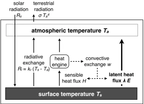
Fig. 1. Schematic illustration of the simple energy balance model that is used to describe the strength of the hydrologic cycle through the rate of surface evaporation,E, with the main variables and fluxes used here. After Kleidon and Renner (2013).
2 Model description
We use the approach of Kleidon and Renner (2013), which describes a thermodynamically consistent global steady state of the surface–atmosphere system in which the hydrologic cycle is represented by evaporation (which balances precip-itation,E=P, in steady state). The layout of the model as well as the main fluxes is shown in Fig. 1. The model uses the surface and global energy balance to describe the surface temperature,Ts, as well as the (atmospheric) radiative
tem-perature,Ta. The surface is assumed to be an open water
sur-face, all absorption of solar radiation is assumed to take place at the surface, and it is assumed that the atmosphere is opaque for terrestrial radiation so that all radiation emitted to space originates from the atmosphere. Atmospheric dynamics, and particularly the turbulent heat fluxes, are not explicitly con-sidered, but rather inferred from the thermodynamic limit of generating convective motion. The important point to note is that for convective exchange to take place in a steady state, motion needs to be continuously generated against inevitable frictional losses. This kinetic energy is generated out of heat-ing differences akin to a heat engine (as shown in Fig. 1). The conversion of heat to kinetic energy by this heat engine is thermodynamically constrained, and such a thermodynamic limit sets the limit to the turbulent exchange at the surface. A brief derivation of this limit from the laws of thermodynam-ics is provided in the Appendix. We will refer to this limit and the associated state of the surface energy balance as the state of maximum power, with power being the physical measure of the rate at which work is being performed. We then mea-sure the strength of the hydrologic cycle by the value ofEat this maximum power state.
In the model, the surface energy balance is expressed as
A. Kleidon and M. Renner: Hydrologic cycling and global climatic change 457
whereRsis the absorbed solar radiation at the surface (which
is prescribed),Rl the net cooling of the surface by
terres-trial radiation,H the sensible heat flux, and λE the latent heat flux. We use simple, but common formulations for these fluxes which are simple enough to obtain analytical results. For the net radiative cooling, we assume a simple linearized form,Rl=kr(Ts−Ta). Here,kris a linearized radiative
“con-ductance” that relates to the strength of the greenhouse ef-fect. The sensible and latent heat fluxes are expressed as tur-bulent exchange fluxes in the form of H=cpρw(Ts−Ta)
and λE=λ ρw(qsat(Ts)−qsat(Ta)). The heat capacity of
air is cpρ= 1.2 ×10³J m−3K−1, with a density of about
ρ= 1.2 kg m−3;w is a velocity which describes the rate of vertical mass exchange and is determined below from the thermodynamic maximum power limit;λ= 2.5×10⁶J K−1 is the latent heat of vaporization; qsat= 0.622esat/p is the
saturation specific humidity;esatis the saturation vapor
pres-sure, andp= 1013.25 hPa is surface air pressure. For the sat-uration vapor pressure, we use the numerical approximation of esat(T )=e0·ea−b/T (Bohren and Albrecht, 1998), with
e0= 611 Pa, a= 19.83 andb= 5417 K and temperatureT in
K. The global energy balance yields an expression for the temperatureTa:
0=Rs −σ Ta4, (2)
whereσ is the Stefan–Boltzmann constant.
The strength of the convective heat fluxes are derived from the assumption that surface exchange is driven mostly by lo-cally generated buoyancy at the surface, and that the power to generate motion by dry convection,H·(Ts−Ta)/Tsis
max-imized. The Carnot limit has a maximum, because a greater value ofH is associated with a smaller value ofTs−Tadue
to the constraint imposed by the surface energy balance. This tradeoff betweenH andTs−Ta results in a distinct state of
maximum power associated with convective exchange at in-termediate values for these two terms (see also Appendix). The maximization is achieved by optimizing the vertical ex-change velocityw. At maximum power, the optimum value for the vertical exchange velocity,wopt, is given by
wopt=
γ
s+γ
Rs
2cpρ (Ts −Ta)
, (3)
where γ= 65 Pa K−1 is the psychrometric constant and s= desat/dTs is the slope of the saturation vapor pressure
curve. This maximum power state results in an energy par-titioning at the surface of
Rl,opt=
Rs
2 Hopt= γ
s+γ Rs
2 λ Eopt= s
s+γ Rs
2 . (4) The expression ofEoptis nearly identical to the equilibrium
evaporation rate (Slayter and McIlroy, 1961; Priestley and Taylor, 1972), a concept that is well established in estimating evaporation rates at the surface, with the additional constraint
that the net radiation of the surface at a state of maximum convective power is half of the absorbed solar radiation,Rs.
This partitioning between radiative and turbulent heat fluxes at the surface is associated with a characteristic tem-perature difference,Ts−Ta, which can be used to infer the
associated temperatures. The radiative temperature of the at-mosphere,Ta, follows directly from the global energy
bal-ance, eqn. 2, and is unaffected by the partitioning:
Ta =
R
s
σ 1/4
. (5)
Surface temperature, Ts, at the maximum power state is
derived from the expression of net radiative exchange, Rl,opt=kr(Ts−Ta)=Rs/2, and is given by
Ts =Ta+
Rs
2kr
. (6)
In Kleidon and Renner (2013), we showed that this model reproduces the global evaporation rate as well as poleward moisture transport very well. It is important to note, how-ever, that the expression for evaporation given by Eq. (4) represents the maximum evaporative flux that is achieved by locally generated motion near the surface only. In practice, the equilibrium evaporation rate is often corrected by the Priestley-Taylor coefficient (Priestley and Taylor, 1972) of ca. 1.26, which can be understood as the effect of horizontal motion that is generated by horizontal differences in absorp-tion of solar radiaabsorp-tion (Kleidon and Renner, 2013). However, as this coefficient simply acts as a multiplier, it does not af-fect the relative sensitivity of evaporation to changes in the surface energy balance. Also note that evaporation driven by local convection by surface heating can already explain more than 70 % of the strength of the present-day hydrologic cy-cle (Kleidon and Renner, 2013). We will therefore consider only this locally driven rate of evaporation in the following derivation of the sensitivities.
3 Results
To derive the hydrologic sensitivity to surface temperature, we are interested in the expression 1/EdE/dTs. We first note
thatTsis not the independent variable of our model, because
Ts=Ts(kr, Rs)with the relationship given by Eq. (6), and
that solar radiative forcing,Rs, and the greenhouse
param-eter,kr, are our independent variables. We can, however, use
Eq. (6) to makeTs andkrour independent variables, andRs
our dependent variable. This sounds a bit backward, but is mathematically sound and allows us to compute 1/EdE/dTs
analytically.
We now use the expression ofEoptin Eq. (4) as the
evap-oration rate to derive the hydrologic sensitivity. This expres-sion depends ons andRs, which are both related to our
1 E
dE dTs
= 1 E
∂E ∂s
ds dTs
+ 1 E
∂E ∂Rs
∂Rs
∂Ts
. (7)
Since∂Rs/∂Ts=(∂Ts/∂Rs)−1, we can also express this as
1 E
dE dTs
= 1 E
∂E ∂s
ds dTs
+ 1 E
∂E ∂Rs
∂T
s
∂Rs
−1
(8) for which the derivative∂Ts/∂Rs can be directly calculated
from Eqs. (6) and (5). We refer to Eq. (8) as the hydrologic sensitivity.
The hydrologic sensitivity consists of two terms. The first term on the right hand side expresses the dependence of evap-oration ons, which depends strongly on surface temperature, while the second term describes the dependence of evapora-tion on the solar radiative forcing, which also affects surface temperature.
When a difference in surface temperature,1Ts, is caused
by changes in the atmospheric greenhouse effect (i.e., a dif-ferent value ofkr), then the solar radiative heating is a
con-stant and 1/EdE/dTs= 1/E ∂E/∂sds/dTs. This sensitivity
represents only a shift in the partitioning between the sensi-ble and latent heat flux, as the overall magnitude of turbulent fluxes does not change sinceRsdoes not change.
If1Ts is caused by a difference inRs, then 1/EdE/dTs
consists of two terms, expressing the change of evaporation due to a change insthat is caused by the increase in temper-ature, but also the overall increase in turbulent fluxes due to the increase inRs. Hence, we would expect different
hydro-logic sensitivities to surface temperature, depending on the type of radiative change. Changes in the greenhouse effect af-fect the first term of the right hand side of Eq. (8) only, while changes in solar radiation affect both terms of the right hand side of Eq. (8) and thus should result in a greater sensitivity. The first term in Eq. (8) expresses the change of evapora-tion,E, to surface temperature,Ts, by altering the value ofs:
1 E
∂E ∂s
ds dTs
= γ
s+γ 1 s
ds dTs
. (9)
We note that this sensitivity does not involve the rela-tive change in saturation vapor pressure 1/esatdesat/dTs,
but rather the relative change in the slope in saturation va-por pressure 1/sds/dTs. The proportionality to the slope
1/sds/dTs, rather than 1/esatdesat/dTs, is due to the fact that
the intensity of the water cycle does not depend onesat(Ts),
but rather on the difference ofesat(Ts)−esat(Ta), which is
approximated in our model by the slopes. Hence, the sensi-tivity of the hydrologic cycle does not follow 1/esatdesat/dT,
but rather 1/sds/dT. The sensitivity is further reduced by a factorγ /(s+γ ), which originates from the energy balance (and maximum power) constraint and ensures thatEis not unbound with much higher values forTs, but converges to an
upper limit ofRs/2.
To quantify this first term of the sensitivity for present-day conditions, we useRs= 240 W m−2 and derive a value
forkr= 3.64 W m−2K−1indirectly from the observed global
mean temperatures, Ts= 288 K and Ta= 255 K and from
Eq. (6) above. With this radiative forcing and values of γ= 65 Pa K−1 and s= 111 Pa K−1, we obtain a numerical value of this sensitivity of
1 E
∂E ∂s
ds dTs
≈2.2 % K−1 (10)
which matches the mean sensitivity of climate models of 2.2 % K−1(Allen and Ingram, 2002; Held and Soden, 2006; Li et al., 2013).
The second term of Eq. (8) is due to a difference in absorp-tion of solar radiaabsorp-tion,1Rs, and is given by
1 E
∂E ∂Rs
· ∂T
s
∂Rs
−1
= 4krσ
1/4
2σ1/4R
s+krR1s/4
. (11)
This sensitivity depends only on radiative properties and re-sults in a sensitivity of
1 E
∂E ∂Rs
· ∂T
s
∂Rs
−1
≈1 % K−1. (12)
This sensitivity is about half the value of the first term when evaluated using present-day conditions, so that the total hy-drologic sensitivity to surface temperature change caused by solar radiation is about 3.2 % K−1and thus exceeds the above sensitivity to changes in the atmospheric greenhouse effect.
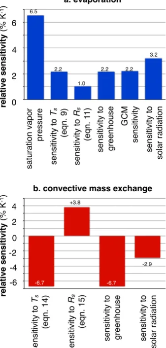
These sensitivities are shown graphically in Fig. 2a. The relative proportion of this sensitivity to that caused by changes in the atmospheric greenhouse is consistent with the proportions reported by Bala et al. (2008) and Andrews et al. (2009). In both studies, the authors reported a sensitivity to surface temperature caused by changes in the atmospheric greenhouse of 1.5 % K−1, while the sensitivity to changes in solar radiation was given as 2.4 % K−1. While the mag-nitude of the sensitivity is smaller compared to the sensitiv-ities calculated here and most other climate models (Allen and Ingram, 2002; Held and Soden, 2006; Li et al., 2013), the sensitivity to temperature differences caused by differ-ences in solar radiation is about 60 % greater than those due to differences in the greenhouse effect, which is similar to the difference that is estimated here.
We will next look at the sensitivities of convective mass exchange that is associated with these differences in hydro-logic cycling. The sensible and latent heat flux are accom-plished by convective motion, which exchanges the heated and moistened air near the surface with the cooled and dried air of the atmosphere. To evaluate the sensitivity of convec-tive motion to surface temperature, we evaluate the relaconvec-tive difference inw in response to a difference inTs, for which
we use the expression ofwoptas given in Eq. (3):
1 w
dw dTs
= 1 w
∂w ∂Ts
+ 1 w
∂w ∂Rs
· ∂T
s
∂Rs
−1
A. Kleidon and M. Renner: Hydrologic cycling and global climatic change 459
0 % 1 % 2 % 3 % 4 % 5 % 6 % 7 %
esat term 2 GCM
4 2 0 6 re la ti v e s e n s iti v ity (% K -1) a. evaporation sa tu ra ti o n va p o r p re ssu re se n si ti vi ty to Ts (e q n . 9 ) se n si ti vi ty to Rs (e q n . 11 ) se n si ti vi ty to g re e n h o u se GCM se n si ti vi ty se n si ti vi ty to so la r ra d ia ti o n 6.5
2.2 2.2 2.2
1.0 3.2 -7 % -5 % -3 % -1 % 1 % 3 % 5 %
term 1 term 2 greenhouse Untitled 1
0 -2 2 re la ti v e s e n s iti v ity (% K -1)
b. convective mass exchange
se n si ti vi ty to Ts (e q n . 1 4 ) se n si ti vi ty to Rs (e q n . 1 5 ) se n si ti vi ty to g re e n h o u se se n si ti vi ty to so la r ra d ia ti o n -6.7 +3.8 -2.9 4 -4 -6 -6.7
Fig. 2. Sensitivity of (a) the hydrologic cycle (evaporationE) and
(b) convective mass exchange (exchange velocityw) to differences
in surface temperature (Ts). Shown are the numerical values for the
relative sensitivities as given in the text for present-day conditions. Also included in (a) is the sensitivity of saturation vapor pressure, 1/esatdesat/dTs, as well as the mean sensitivity to greenhouse
dif-ferences reported for climate models by Held and Soden (2006) (“GCM sensitivity”).
As in the case of evaporation, the sensitivity consists of two terms, with the first term representing the direct response of wtosandTs. This first term is given by
1 w
∂w ∂Ts
= − s s+γ
1 s
ds dTs
− 1
Ts −Ta
. (14)
Using the values from above, this yields a sensitivity of −6.7 % K−1. The sensitivity is negative, implying that con-vective mass exchange is reduced by a stronger greenhouse effect. This sensitivity is consistent with previous interpre-tations as described by Betts and Ridgway (1989) and Held and Soden (2006), and the estimates of about 4–8 % reported by Boer (1993).
The second term in Eq. (13) describes the indirect effect of differences in solar radiation onwthrough differences in Ts:
1 w ∂w ∂Rs · ∂Ts ∂Rs −1
= kr+
k2
r
2σ1/4R7/4 s
!
· 4krσ
1/4
2σ1/4R
s+krRs1/4
.(15)
This expression yields a sensitivity of +3.8 % K−1, so that the total sensitivity of convective mass exchange to tempera-ture differences caused by differences in absorption of solar radiation is−2.9 % K−1. This sensitivity is noticeably less than the sensitivity to changes in the atmospheric greenhouse effect (see also Fig. 2b).
In summary, we have shown here that our analytical ex-pressions for the sensitivity of evaporation rate, Eq. (9), can reproduce the reported mean sensitivity of climate models to greenhouse-induced temperature differences. Due to an addi-tional term that relates to changes in absorbed solar radiation (Eq. 11), the hydrologic sensitivity is greater when the tem-perature increase is due to an increase in the absorption of solar radiation, which is also consistent with what is reported from climate model studies. Associated with these changes in the hydrologic cycle are changes in the intensity of verti-cal mass exchange, which depend on the type of change in the radiative forcing. Hence, our approach appears to repre-sent a simple yet consistent way to capture the mean aspects of climate change that are reflected in surface temperature differences.
4 Discussion
Before we interpret our results in more detail, we first dis-cuss some of the limitations of our approach and evaluate the extent to which these affect the results. We then interpret our results for the hydrologic sensitivity and relate this in-terpretation to previous explanations. We close with a brief discussion of one of the implications of our work for the cli-matic impacts of climate geoengineering by solar radiation management.
4.1 Limitations
Naturally, we have made a number of assumptions in our approach. These assumptions relate to the assumption of (a) the maximum power limit for convective exchange, (b) a steady state of the energy balances, (c) surface exchange be-ing caused by local heatbe-ing, and (d) a simple treatment of processes in our model.
avoids this empirical parameter. This limit relates closely to the hypothesis that atmospheric motion maximizes material entropy production, noting that in steady state, power equals dissipation, and entropy production is described by dissipa-tion divided by temperature. This hypothesis was first pro-posed by Paltridge (1975), and has been quite successful, for instance in predicting heat transport in planetary atmospheres (Lorenz et al., 2001), in deriving an empirical parameter re-lated to turbulence in a general circulation model (Kleidon et al., 2003), and other applications in climate science (e.g., Ozawa et al., 2003). Hence, the assumption that atmospheric motion operates near such a thermodynamic limit, while not widely recognized, has considerable support. For the deriva-tion of our sensitivities, this assumpderiva-tion only matters to the extent that it predicts that net radiation does not change in the case of greenhouse-induced warming. In other words, the derivation of the hydrologic sensitivity to greenhouse-induced warming (Eq. 9) could have been done with the as-sumption that net radiation does not change. Likewise, the hydrologic sensitivity to solar-induced changes of surface temperature (Eqs. 9 and 11) could have been derived from the assumption that the ratio between radiative and turbulent cooling remains fixed. Both of these assumptions can then be justified and explained by the maximum power limit.
We also assumed that the energy balances of the sur-face and the atmosphere are in a steady state. This assump-tion ignores the temporal variaassump-tions on diurnal and seasonal timescales, which result in the dynamics of boundary layer growth and changes in heat storage. These aspects are most relevant on land, while over the ocean, these aspects are likely to play a minor role due to the large heat capacity of water. Since the sensitivity of the hydrologic cycle is domi-nated by the oceans, it would thus seem reasonable to neglect these variations.
Another assumption that we have made is that the turbu-lent exchange at the surface results only from local surface heating. This assumption neglects the fact that the large-scale circulation adds extra turbulence to the surface, thus gener-ating more turbulence at the surface than what would be ex-pected by local heating alone. This extra contribution would shift the partitioning in the surface energy balance towards turbulent heat fluxes. In the framework of the equilibrium evaporation rate, this shift can be interpreted by the Priestley-Taylor coefficient. We incorporated this effect in Kleidon and Renner (2013) by introducing a factor into the formulation of the sensible and latent heat flux, but we did not use this factor here. The reason for omitting this factor is that as long as this factor is independent ofTs, the relative sensitivities that we
derived here are not affected as this factor would cancel out. Hence, this large-scale contribution to turbulent exchange is unlikely to result in substantially different sensitivities.
In addition, we implemented processes in our approach in a simplified way. We assumed that all absorption of solar ra-diation takes place at the surface, while observations (e.g., Stephens et al., 2012) state that it is only about 165 W m−2
rather than 240 W m−2of solar radiation which is absorbed
at the surface. We used this simplification to keep the model as simple as possible (otherwise, we would need to account for atmospheric absorption in the expression forTa). For the
hydrologic sensitivity, this simplification plays a minor role because the sensitivity is formulated in relative terms, which is independent ofRs (at least the first term in Eq. 8). In
ad-dition, we assumed that the atmosphere is mostly opaque for terrestrial radiation. This assumption does not hold for all re-gions. Particularly in dry and cold regions, the atmosphere is more transparent to terrestrial radiation. This would affect our model in which it is assumed that all terrestrial radiation to space originates from the atmosphere (cf. Eq. 2).
Overall, while we made several assumptions and simplifi-cations in obtaining our results, it would seem that our results are rather robust. These assumptions may need to be revis-ited and refined when using this approach at different scales or conditions. For instance, when this approach is applied to land, then one would need to account for the additional con-straint of water limitation. When it is applied to the diurnal cycle, one would clearly need to account for changes in heat storage. These factors can, of course, be included in an exten-sion of the approach, but they should nevertheless not affect our results at the global scale in the climatic mean.
4.2 Interpretation
The interpretation of our results is relatively straightforward and can be attributed entirely to changes in the surface en-ergy balance. This focus on changes in the surface enen-ergy balance is plausible, because after all, convective mass ex-change, the associated transport of sensible and latent heat, and hence hydrologic cycling is caused by surface heating. It is important to note that the actual heating of the surface is solely due to the absorption of solar radiation,Rs, while
terrestrial radiation,Rl, cools the surface. In the following,
we explain these changes and illustrate these for an example of a surface warming of1Ts= 2 K, which is shown in Fig. 3.
When the surface warming is entirely caused by an in-crease of the atmospheric greenhouse effect,Rsis effectively
unchanged, but the cooling of the surface by terrestrial ra-diation is less efficient. In our model, this reduced cooling efficiency is reflected in a lower value ofkr. This lower value
ofkr, however, does not affect the partitioning of absorbed
solar radiation into radiative and turbulent cooling, Rl and
H+λE, at the maximum power state. This is noticeable in Eq. (4), since the partitioning does not depend on the value ofkr. Hence,RsandRldo not change (cf. Fig. 3, blue bars).
However, becausekris reduced, it requires a greater
temper-ature difference, Ts−Ta, to accomplish the same radiative
cooling flux,Rl. SinceTais fixed by the global energy
bal-ance and is independent ofkr, this can only be accomplished
by an increase inTs. This surface warming is then associated
A. Kleidon and M. Renner: Hydrologic cycling and global climatic change 461
-6 -4 -2 0 2 4 6
-1.7 -0.8
-2.5
-5.0
4.8
-2.3 2.5
5.0
3.2
-3.2 0.0
0.0 PD +2K (kr) +2K
(Rs) GEO Rs (W m-2) 240 240 0.00 245 5.00 235.00 -5.00
Ts (K) 288 290 2.00290.00 2.00 287.93 -0.07 Ta (K) 255 255 0.00256.39 1.32 253.73 -1.34 s (Pa K-1) 110.77124.3813.61124.41 13.64 110.34 -0.43 kr(W m-2
K-1)
3.64 3.44 -0.21 3.64 0.00 3.44 -0.21 Rl,u (W m-2) 390 401 10.95 401 10.97 390 -0.36 Rl,d (W m-2) 270 281 10.95 279 8.47 272 2.14 Rl (W m-2) 120 120 0.00 122.5 2.50 117.5 -2.50 H (W m-2) 44 41 -3.19 42 -2.34 44 -0.82 λE (W m-2) 76 79 3.19 80 4.84 74 -1.68 w (mm s-1) 1.12 0.98 -0.14 1.04 -0.08 1.06 -0.06
a
b
so
rb
e
d
so
la
r
ra
d
ia
tio
n
,
Rs
d
iffe
re
n
c
e
(W
m
-2)
n
e
t
te
rre
st
ri
a
l
ra
d
ia
tio
n
,
Rl
se
n
si
b
le
h
e
a
t
flu
x,
H
la
te
n
t
h
e
a
t
flu
x, λE
warming by greenhouse warming by solar radiation solar geoengineering
Fig. 3. Estimates of the changes in the surface energy balance components due to a warming of 1Ts= 2 K caused by an
in-crease in the atmospheric greenhouse effect (blue, “warming by greenhouse”), by an increase in absorbed solar radiation (red, “warming by solar absorption”), and when a greenhouse warm-ing of 2 K is compensated for by a reduction of solar radiation by some geoengineering management (yellow, “solar geoengineer-ing”). The numbers are obtained using values ofRs= 240 W m−2
andkr= 3.64 W m−2K−1for the present-day climate, a reduction
ofkrtokr= 3.44 W m−2K−1to get a surface warming of 2 K by
changes in the greenhouse effect, an increase of1Rs= 5 W m−2
to get a surface warming of 2 K by changes in absorption of so-lar radiation, and a combined change ofkr= 3.44 W m−2K−1and
1Rs=−5 W m−2 to implement the solar radiation management
effects.
has a greater value at a warmer temperature, resulting in a greater proportion,s/(s +γ ), of the turbulent cooling be-ing represented by the latent heat flux, thus resultbe-ing in a stronger hydrologic cycle (Fig. 2a). In the example shown in Fig. 3 the consequence of the warming is reflected merely in the shift from the sensible heat flux to the latent heat flux, but the magnitude of both does not change.
Since the difference Ts−Ta is enhanced, the turbulent
heat fluxes are accomplished by less convective mass ex-change, which results in the negative sensitivity 1/w ∂w/∂Ts
(Fig. 2b). Since both sensitivities deal with the intensity of convective transport and its partitioning into sensible and la-tent heat, the sensitivities are expressed only in terms of re-lated properties (s,γ,Ts−Ta, cf. Eqs. 9 and 14), but do not
depend explicitly on radiative properties of the system (Rs,
kr). This interpretation is consistent with the general
under-standing of the greenhouse effect, but it emphasizes that the atmospheric greenhouse effect acts to reduce the efficiency by which the surface cools through the emission of terres-trial radiation.
The situation is different when the surface warms due to enhanced absorption of solar radiation (Fig. 3, red bars). In this case, the surface is heated more strongly (Rs is
in-creased), so the rate of cooling,Rl+H+λE, is increased
as well. Apart from the difference in surface temperature and the associated differences in the partitioning between the sen-sible and latent heat flux, the overall magnitude of the turbu-lent fluxes is altered as well. Hence, the sensitivity is greater than in the case of greenhouse warming, which is noticeable in our example by the increase in sensible and latent heat (compare red vs. blue bars in Fig. 3). The additional con-tribution by the overall increase in turbulent fluxes depends onRsand on the temperature difference, which depends on
Rs andkr. Consequently, the second term in the sensitivities
depends explicitly on the radiative properties of the system (Rs,kr, cf. Eqs. 11 and 15). This enhancement of the
turbu-lent fluxes favors greater convective mass exchange, so that the sensitivity of convective mass exchange is reduced com-pared to differences caused by a stronger greenhouse effect.
Our interpretation is quite different from the common ex-planation for the hydrologic sensitivity (e.g., Mitchell et al., 1987; Allen and Ingram, 2002; Takahashi, 2009; Allan et al., 2013). The common explanation starts by considering the at-mospheric energy balance. Surface warming results in a per-turbation of this energy balance. It accounts for the extra re-lease of latent heat, λ1P, the change in radiative cooling of the atmosphere to space,1Rtoa, the change in radiative
fluxes from the surface, 1Rl, and a change in the sensible
heat flux,1H:
λ1P =1Rtoa−1Rl−1H. (16)
The common explanation for the lower sensitivity of precip-itation to surface warming compared to the sensitivity of the saturation water pressure argues that the additional release of latent heat,λ1P, is constrained by the ability to radiate away the additional heat by the term1Rtoa−1Rl. The term1H
in these considerations is commonly neglected becauseHis quite a bit smaller than the latent heat flux.
This energy balance is, of course, indirectly also obeyed in our model even though we do not explicitly consider it. First, we consider a steady state, so that 1Rs=1Rtoa,
λ1P=λ1E, and, 1/P·dP /dTs= 1/E·dE/dTs.
We first consider the case of greenhouse-induced sur-face warming. In this case, changes in the greenhouse effect do not change the radiative temperature of the atmosphere (which is entirely determined byRs, Eq. 5), hence,1Rtoa= 0.
The termRldoes not change either, because the surface
heat-ing by solar radiation did not change (1Rs= 0) and the
maxi-mum power constraint results in an equal partitioning among RlandH+λE, no matter how strong the greenhouse effect
is. Hence, the overall changes in the atmospheric energy bal-ance reduce to
This implies that the weak, 2.2 % K−1increase in the strength
of the hydrologic cycle can simply be explained by the re-duction of the sensible heat flux at the surface. This inter-pretation is identical to what we found for the changes in the surface energy balance: a greenhouse-induced surface warm-ing merely affects the partitionwarm-ing between sensible and la-tent heat, but does not affect the magnitude of the turbulent heat fluxes (see also example in Fig. 3, blue bars). This ex-planation is different to the common exex-planation, which ne-glects changes in the sensible heat flux. In our explanation, the hydrologic sensitivity due to greenhouse-induced surface warming is entirely due to the reduction ofH.
The changes in the atmospheric energy balance are dif-ferent if the surface temperature change was caused by changes in solar radiation. If absorbed solar radiation in-creases by1Rs, then the global energy balance requires that
1Rtoa=1Rs, so that the radiative temperatureTa must
in-crease. The partitioning of energy at the surface changes as well. At a state of maximum power, the additional heating of1Rsresults in an equal increase in radiative and turbulent
fluxes of1Rl=1Rs/2, and of1(H +λE)=1Rs/2. In
ad-dition, the increase in surface temperature alters the partition-ing betweenHandλE. Hence, in this case, all four terms are going to change in Eq. (16), which is quite a different change than the greenhouse-induced warming.
Overall, our explanation is quite different to the common explanation of the hydrologic sensitivity. Yet, our explana-tion is simple, physically based, consistent with the atmo-spheric energy balance, and predicts the right value of the sensitivities.
4.3 Implications
An important implication of our interpretation of the hydro-logic sensitivity is that the forcing of the surface cannot be simply lumped into a single, radiative forcing concept. The notion of a “radiative forcing” combines the changes in solar and terrestrial radiation into one variable. However, as these sensitivities show, solar radiation plays a very different role than terrestrial radiation. The strength of hydrologic cycling as well as convective mass exchange react quite differently if the surface is warmed due to stronger heating by solar ra-diation or due to a weaker cooling by a stronger greenhouse effect. An immediate consequence of this notion is that cli-mate geoengineering cannot simply be used to undo global warming (see also Bala et al., 2008 and Tilmes et al., 2013). This can be illustrated using the sensitivities given above.
We consider the case of surface warming of 2 K caused by an enhanced greenhouse effect, as before, except that we look at the relative sensitivities rather than the absolute changes in the surface energy balance. Since this increase of surface temperature is caused by the greenhouse effect, the hydrologic cycle would be strengthened by the sensitivity 1/E ∂E/∂sds/dTs(Eq. 9 and blue bars in Fig. 3). This
sen-sitivity has a value of 2.2 % K−1, so thatE would increase
−10
−5 0 5 10
−4 −3 −2 −1 0 1 2 3 4
B
C
∆T = 2K
D
iffe
re
n
c
e
i
n
Ev
a
p
o
ra
ti
o
n
(%
)
Difference in Temperature (K)
A ∆E/E = 4.4%
∆E/E = -6.4% ∆T = 2K
2.2 % K
-1
3.2% K -1
a. evaporation
−20
−10
0 10 20
−4 −3 −2 −1 0 1 2 3 4
B C
∆T = 2K
D
iffe
re
n
c
e
i
n
Ex
c
h
a
n
g
e
(%
)
Difference in Temperature (K) A
∆w/w = -13.4%
∆w/w = +5.8%
∆T = 2K
-6 .7 %
K-1
-2.9% K-1
b. convective mass exchange
Fig. 4. Illustration of the contrary effects of greenhouse vs. solar-induced changes on (a) evaporation,E, and (b) convective mass exchange, w. The sensitivity of evaporation to a surface warm-ing of1Ts= 2 K by an elevated greenhouse effect results in an
in-crease of 2.2 % K−1, resulting in a change from point A to B (blue line). A geoengineering response aimed at compensating this in-crease in surface temperature by reducing solar radiation would change evaporation at a rate of 3.2 % K−1, resulting in a change from point B to C (red line). Likewise, the surface warming would decrease the vertical exchange velocity,w, by−6.7 % K−1(point A to B), while the geoengineering response would increase it at a rate of 2.9 % K−1(point B to C). Hence, while the geoengineering re-sponse may undo differences in surface temperature, it cannot com-pensate changes in the hydrologic cycle and vertical mass exchange at the same time.
by 4.4 % with a warming of 2 K. This increase is shown by the arrow in Fig. 4a from the original climatic state “A” to the state in which the surface is heated by 2 K (point “B”). The convective mass exchange would be reduced following the sensitivity 1/w ∂w/∂Ts (Eq. 14), which has a value of
−6.7 % K−1. With a 2 K warming, the convective mass ex-change would be reduced by 13.4 % (Fig. 4b).
A. Kleidon and M. Renner: Hydrologic cycling and global climatic change 463
by some geoengineering schemes, then the value ofRswould
change and we need to consider both terms in the sensitiv-ities of evaporation (Eq. 8) and convective mass exchange (Eq. 13). The hydrologic cycle would be reduced not at a rate of 2.2 % K−1as in the case above, but rather at the combined value of 3.2 % K−1, which includes the additional sensitivity given by Eq. (11). Hence, with a cooling of 2 K that would be necessary to undo the surface warming, the strength of the hydrologic cycle would be reduced in total by 6.4 %. This is shown in Fig. 4a by the arrow from point B to C. Overall, the warming would be undone, but the strength of the hydro-logic cycle at this state of geoengineering (point C) would be weaker by 2 % compared to the original state (point A). Likewise, the sensitivities of convective mass exchange do not compensate either. The cooling of 2 K by the reduction of absorbed solar radiation follows the weaker sensitivity of −2.9 % K−1, so that the convective mass exchange would
in-crease by only 5.8 % (see arrow from point B to C in Fig. 4b). Hence, overall, the greenhouse warming by 2 K and the geo-engineering cooling by 2 K would weaken convective mass exchange by 6.8 % (compare point A and C in Fig. 4b, which is also seen in the yellow bars in Fig. 3).
Hence, such intervention by geoengineering may undo surface warming, but it cannot undo differences in hydro-logic cycling and convective mass exchange at the same time. What this tells us is that it is important to consider the differ-ent roles of solar and terrestrial radiation separately in future studies on the strength of the hydrologic cycle and global cli-matic change (see also Jones et al., 2013).
5 Summary and conclusions
In this study we showed that the sensitivity of the hydro-logic cycle to surface temperature can be quantified using a simplified surface energy balance and the assumption that convective exchange near the surface takes place at the limit of maximum power. This model yields analytical expres-sions for the hydrologic sensitivity and shows that it does not scale with the saturation vapor pressure, but rather with its slope. The hydrologic sensitivity scales with the slope of the saturation vapor pressure curve because hydrologic cy-cling relates to the differences in saturation vapor pressure between the temperatures at which evaporation and conden-sation takes place. This difference is approximated by the slope. The actual sensitivity is then further reduced by a fac-torγ /(s+γ ), which originates from the surface energy bal-ance constraint. Our analytical expressions also show that surface warming caused by increases in absorbed solar ra-diation result in a greater sensitivity of the hydrologic cy-cle than warming caused by an increased greenhouse effect. This greater sensitivity for warming due to solar radiation is simply explained by the requirement for a greater total cool-ing rate by radiative and turbulent fluxes. Even though our approach is highly simplistic and omits many aspects, the
analytical expressions yield sensitivities that are consistent with those found in rather complex climate models. We con-clude that the hydrologic sensitivity to surface warming can be explained in simple, physical considerations of the surface energy balance.
An important implication of our results is that geoengi-neering approaches to reduce global warming are unlikely to succeed in restoring the original climatic conditions. Be-cause of the difference in hydrologic sensitivities to solar vs. greenhouse induced surface warming, the changes in hydro-logic cycling and convective mass exchange do not compen-sate even if surface temperature changes are compencompen-sated by solar radiation management. This example emphasizes the different roles that solar and terrestrial radiation play in the surface energy balance and challenges the frequently used ra-diative forcing concept, which lumps these two components together. It would seem insightful to extend our study in the future to other aspects of global climatic change, in which the different roles in solar and terrestrial radiation are explicitly considered in a thermodynamically consistent way.
Appendix A
Thermodynamic limits
The first and second law of thermodynamics set a fundamen-tal direction as well as limits to energy conversions within any physical system. We apply it here to derive the limit to how much kinetic energy can be derived from the differen-tial radiative heating between the surface and the atmosphere. The following derivation summarizes Kleidon and Renner (2013).
To derive the limit, we consider a heat engine as marked in Fig. 1 that is driven by the sensible heat flux,H. In the steady-state setup used here, the first law of thermodynamics requires that the turbulent heat fluxes in and out of the engine, HandHout, are balanced by the generation of kinetic energy,
G:
0=H −Hout−G. (A1)
The second law of thermodynamics requires that the entropy of the system does not decrease during the process of gen-erating kinetic energy. This requirement is expressed by the entropy fluxes associated with the heat fluxes H andHout
that enter and leave the heat engine at the temperatures of the surface and the atmosphere:
H Ts
− Hout Ta
≥ 0. (A2)
In the best case, the entropy balance equals zero, which then allows us to express the fluxHoutas a function ofH,Ts, and
Hout =H ·
Ta
Ts
. (A3)
When combined with Eq. (A2), this yields the well-known Carnot limit of the power generated by a heat engine: G=H · Ts −Ta
Ts
. (A4)
In steady state, this generated power is dissipated by friction, so thatG=D.
While the Carnot limit provides a constraint on how much power can be generated, it does not directly provide a limit on the value ofH. Such a limit is obtained when we consider that the temperature difference,Ts−Ta, is not independent of
H, but rather constrained by the energy balance (Eq. 1). This temperature difference can be expressed using the expression for the net radiative exchange flux,Rl, from above as
Ts−Ta =
Rs−H −λE
kr
. (A5)
Hence, the surface energy balance demands that the tempera-ture difference,Ts−Ta, decreases with an increasing value of
H. When combined, this yields an expression for the Carnot limit of
G=H · Rs−H −λE kr
. (A6)
Due to the contrasting effects ofHonGin the two terms of the right hand side, the Carnot limit has a maximum value at intermediate values ofH.
We obtain this maximum in the Carnot limit when we first use the formulation of the sensible and latent heat flux from above in terms of the vertical velocity,wto express the tem-perature difference:
Ts−Ta =
Rs
kr+cpρw(1+s/γ )
, (A7)
and then combine this expression with the formulation of the sensible heat flux, which yields:
G= cpρw
Ts kr+cpρw(1+s/γ )2
·R2s. (A8)
This equation has a maximum value with respect tow, which can be derived analytically when we neglect thatTs in the
denominator depends on H as well. The maximization is achieved by ∂G/∂w= 0. This yields the expression of the optimum exchange velocity (Eq. 3) and results in an optimal energy partitioning as given by Eq. (4).
This maximum power limit describes the upper thermody-namic limit by which convective motion can be generated to sustain the sensible heat flux out of local radiative heating by absorption of solar radiation at the surface. It does not nec-essarily imply that this limit is achieved. This would rather
formulate a hypothesis, namely, that the surface-energy par-titioning would operate near this maximum power limit. This hypothesis is very closely related to the proposed princi-ple of Maximum Entropy Production (MEP, Ozawa et al., 2003; Kleidon et al., 2010), noting that in steady state,P=D, and entropy production is described byD/T. A more com-plete discussion on this relationship is given in Kleidon and Renner (2013). In this paper, we assume that natural pro-cesses operate at this thermodynamic limit to derive the ana-lytical expressions.
Acknowledgements. We thank two anonymous reviewers, R. P. Allan, Amilcare Porporato and Michael Roderick for con-structive comments on this manuscript. A. Kleidon acknowledges financial support from the Helmholtz Alliance “Planetary Evolu-tion and Life”. This research contributes to the “Catchments As Organized Systems (CAOS)” research group funded by the German Science Foundation (DFG).
Edited by: M. Sivapalan
References
Allan, R. P., Liu, C., Zahn, M., Lavers, D. A., Koukouvagias, E., and Bodas-Salcedo, A.: Physically consistent responses of the global atmospheric hydrologic cycle in models and observations, Surv. Geophys., doi:10.1007/s10712-012-9213-z, in press, 2013. Allen, M. R. and Ingram, W. J.: Constraints on future changes in
climate and the hydrologic cycle, Nature, 419, 224–232, 2002. Andrews, T., Forster, P. M., and Gregory, J. M.: A surface energy
perspective on climate change, J. Climate, 22, 2557–2570, 2009. Bala, G., Duffy, P. B., and Taylor, K. E.: Impact of geoengineering schemes on the global hydrologic cycle, P. Natl. Acad. Sci. USA, 105, 7664–7669, 2008.
Betts, A. K. and Ridgway, W.: Climatic equilibrium of the atmo-spheric convective boundary layer over a tropical ocean, J. At-mos. Sci., 46, 2621–2641, 1989.
Boer, G. J.: Climate change and the regulation of the surface mois-ture and energy budgets, Clim. Dynam., 8, 225–239, 1993. Bohren, C. F. and Albrecht, B. A.: Atmospheric Thermodynamics,
Oxford Univ. Press, New York, 1998.
Boos, W. R.: Thermodynamic scaling of the hydrologic cycle of the Last Glacial Maximum, J. Climate, 25, 992–1006, 2012. Govindasamy, B., Caldeira, K., and Duffy, P. B.: Geoengineering
Earth’s radiation balance to mitigate climate change from a qua-drupling of CO2, Global Planet. Change, 37, 157–168, 2003. Held, I. M. and Soden, B. J.: Robust responses of the hydrological
cycle to global warming, J. Climate, 19, 5686–5699, 2006. Jones, A. D., Collins, W. D., and Torn, M. S.: On the additivity of
radiative forcing between land use change and greenhouse gases, Geophys. Res. Lett., 40, 4036–4041, doi:10.1002/grl.50754, 2013.
A. Kleidon and M. Renner: Hydrologic cycling and global climatic change 465
Kleidon, A., Fraedrich, K., Kunz, T., and Lunkeit, F.: The atmo-spheric circulation and states of maximum entropy production, Geophys. Res. Lett., 30, 2223, doi:10.1029/2003GL018363, 2003.
Kleidon, A., Malhi, Y., and Cox, P. M.: Maximum entropy pro-duction in environmental and ecological systems, Philos. T. Roy. Soc. B, 365, 1297–1302, 2010.
Li, G., Harrison, S. P., Bartlein, P. J., Izumi, K., and Prentice, I. C.: Precipitation scaling with temperature in warm and cold cli-mates: An analysis of CMIP5 simulations, Geophys. Res. Lett., 40, 4018–4024, doi:10.1002/grl.50730, 2013.
Lorenz, R. D., Lunine, J. I., Withers, P. G., and McKay, C. P.: Titan, Mars and Earth: Entropy production by latitudinal heat transport, Geophys. Res. Lett., 28, 415–418, 2001.
Lunt, D. J., Ridgwell, A., Valdez, P. J., and Seale, A.: “Sun-shade World”: A fully coupled GCM evaluation of the climatic impacts of geoengineering, Geophys. Res. Lett., 35, L12710, doi:10.1029/2008GL033674, 2008.
Mitchell, J. F. B., Wilson, C. A., and Cunnington, W. M.: On CO2 climate sensitivity and model dependence of results, Q. J. Roy. Meteorol. Soc., 113, 293–322, 1987.
Ozawa, H., Ohmura, A., Lorenz, R. D., and Pujol, T.: The second law of thermodynamics and the global climate system – A review of the Maximum Entropy Production principle, Rev. Geophys., 41, 1018, doi:10.1029/2011WR011264, 2003.
Paltridge, G. W.: Global dynamics and climate – a system of mini-mum entropy exchange, Q. J. Roy. Meteorol. Soc., 101, 475–484, 1975.
Priestley, C. H. B. and Taylor, R. J.: On the assessment of surface heat flux and evaporation using large-scale parameters, Mon. Weather Rev., 100, 81–92, 1972.
Slayter, R. O. and McIlroy, I. C.: Practical Micrometeorology, CSIRO, Melbourne, Australia, 310 pp., 1961.
Stephens, G. L., Li, J., Wild, M., Clayson, C. A., Loeb, N., Kato, S., L’Ecuyer, T., Stackhouse, P. W., Lebsock, M., and Andrews, T.: An update on Earth’s energy balance in light of the latest global observations, Nat. Geosci., 5, 691–696, 2012.
Takahashi, K.: Radiative constraints on the hydrological cycle in an idealized radiative-convective equilibrium model, J. Atmos. Sci., 66, 77–91, 2009.