www.earth-syst-dynam.net/3/97/2012/ doi:10.5194/esd-3-97-2012
© Author(s) 2012. CC Attribution 3.0 License.
Earth System
Dynamics
On the determination of the global cloud feedback from satellite
measurements
T. Masters
School of Engineering and Applied Science, UCLA, Los Angeles, California, USA
Correspondence to: T. Masters ([email protected])
Received: 21 January 2012 – Published in Earth Syst. Dynam. Discuss.: 3 February 2012 Revised: 2 August 2012 – Accepted: 7 August 2012 – Published: 23 August 2012
Abstract. A detailed analysis is presented in order to
deter-mine the sensitivity of the estimated short-term cloud feed-back to choices of temperature datasets, sources of top-of-atmosphere (TOA) clear-sky radiative flux data, and tempo-ral averaging. It is shown that the results of a previous analy-sis, which suggested a likely positive value for the short-term cloud feedback, depended upon combining all-sky radiative fluxes from NASA’s Clouds and Earth’s Radiant Energy Sys-tem (CERES) with reanalysis clear-sky forecast fluxes when determining the cloud radiative forcing (CRF). These results are contradicted when1CRF is derived using both all-sky and clear-sky measurements from CERES over the same pe-riod. The differences between the radiative flux data sources are thus explored, along with the potential problems in each. The largest discrepancy is found when including the first two years (2000–2002), and the diagnosed cloud feedback from each method is sensitive to the time period over which the re-gressions are run. Overall, there is little correlation between the changes in the1CRF and surface temperatures on these timescales, suggesting that the net effect of clouds varies during this time period quite apart from global temperature changes. Given the large uncertainties generated from this method, the limited data over this period are insufficient to rule out either the positive feedback present in most climate models or a strong negative cloud feedback.
1 Introduction
The cloud feedback is one of the largest sources of uncer-tainty when trying to determine the global surface temper-ature response to a doubling of CO2, and is the primary
discrepancy leading to differing climate sensitivities in the
global climate models (Bony et al., 2006; Bender, 2011). While many improvements have been made in the way the cloud radiative forcing can be estimated and constrained (Al-lan, 2011), the response of this net cooling effect of clouds to temperature changes (that is, whether the cooling effect becomes stronger or weaker as the climate warms) still re-mains largely uncertain. Within the context of this paper, we use the typical notion of a cloud feedback, whereby it is con-sidered negative if the amount of radiation escaping to space due to clouds (either by reflecting more solar radiation, or al-lowing more outgoing longwave radiation – OLR – through the atmosphere) increases with an increase in temperature, and positive if an increase in temperature results in the oppo-site, thereby exacerbating the warming. All radiative fluxes presented in this paper are thus shown with a positive value indicating a downward flux towards the surface, including CRF and1Rcloud.
2 Data and methods
The CRF is determined by the difference between all-sky and clear-sky radiative fluxes at the top of the atmosphere. A simple examination of the change in CRF with respect to a temperature change (dCRFdT ) would at first appear to give an estimate of the cloud feedback. However, there are sev-eral other climate components that correlate with tempera-ture (surface albedo, water vapor, and the Planck response), which will cause a change in the measured CRF even when no cloud properties have changed (Soden et al., 2008; Shell et al., 2008). Section 2.4 contains details on how the influence of these non-cloud components is removed from the calcu-lated1CRF, yielding1Rcloud. Nonetheless, it is clear that
the method of determining1CRF – and, in particular, the
choice for clear-sky flux – is of primary importance when calculating the cloud feedback in this manner.
2.1 All-sky radiative fluxes
For all-sky TOA fluxes (Fig. 1a), we use CERES Single Scanner Footprint (SSF) 1◦global means (CERES SSF1deg-lite Ed2.6) (Wielicki et al., 1998; Loeb et al., 2012). We have chosen the CERES SSF1 degree product for consistency with Dessler (2010), and because it is more stable with respect to anomalies than its Energy Balanced and Filled (EBAF) counterpart. This is due to the EBAF product supplementing CERES measurements with those from geostationary satel-lites, which improves diurnal coverage, but introduces arti-facts from the GEO data that can result in spurious jumps or trends in the interannual, deseasonalized anomalies (Loeb et al., 2009).
There are two periods over which we perform the analy-sis: the Terra period (Table 1), stretching from March 2000 to June 2011, during which time we use the measurements from the CERES instrument aboard the Terra satellite; and the Aqua period (Table 2), from September 2002 to June 2011, during which we average the CERES products coming from the different Terra and Aqua satellites. For each analysis, we calculate anomalies relative to their respective time intervals. We note that the CERES measurements aboard Aqua actu-ally begin in July 2002, but the relevant data from the At-mospheric Infrared Sounder (AIRS) instrument aboard the same satellite are only available beginning in September of that year.
2.2 Clear-sky radiative fluxes
We use multiple sources of clear-sky radiative fluxes in order to determine the sensitivity to each choice. A time series of the fluxes from the different data products below can be seen in Figs. 1b and 2.
2.2.1 CERES clear-sky
Similar to all-sky fluxes, we use CERES clear-sky fluxes from aboard the Terra satellite over the longer period analy-sis, and then average the data products during the overlapping Terra and Aqua interval. There are, however, several poten-tial issues with using the CERES clear-sky fluxes to deter-mine the CRF that must be considered. For one, there is a known clear-sky sampling bias for OLR in absolute CERES CRF measurements (Cess and Potter, 1987; Sohn and Ben-nartz, 2008), as the observations made over areas during clear-sky conditions coincide with less water vapor in that area. The difference between all-sky and clear-sky fluxes thus aliases some of the OLR trapping properties of the water va-por in with the LW CRF. We note here that, if the bias is sig-nificant in affecting the changes in1CRF (rather than sim-ply in the absolute calculation), a rise in temperature would likely lead to increasing water vapor that traps more OLR,
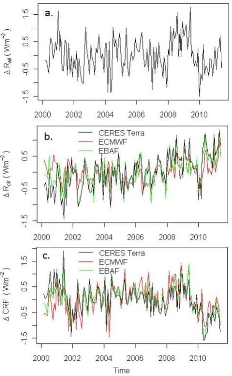
Fig. 1. (a) Global average monthly anomalies for all-sky TOA
ra-diative flux from CERES measurements aboard the Terra satel-lite. (b) Global average monthly anomalies for clear-sky TOA radiative fluxes from CERES Terra, ECMWF ERA-Interim, and CERES EBAF. (c) The global average monthly CRF anoma-lies from CERES-only measurements, CERES-ECMWF, and CERES-EBAF.
which will then appear to bias the LW component towards a more positive cloud feedback. However, modeling of this clear-sky sampling bias indicates it has little impact on the interannual anomalies (Allan et al., 2003). Such a bias would be insignificant for the shortwave component, although there may be a similar absolute sampling bias resulting from differ-ences in aerosol concentration between clear-sky and cloudy scenes (Erlick and Ramaswamy, 2003).
Fig. 2. (a) Global monthly anomalies for shortwave, clear-sky TOA
radiative flux from CERES (Terra + Aqua SSF1 degree), ECMWF ERA-Interim, and CERES EBAF. (b) Global monthly anoma-lies for longwave, clear-sky TOA radiative fluxes from CERES (Terra + Aqua SSF1 degree), ECMWF ERA-Interim, AIRS, and CERES EBAF. (c) Surface temperature anomalies from GISS, ECMWF ERA-Interim 2-m and skin temperatures.
considered clear or cloudy, and misidentification would lead to biases in the reported CERES observations. We note that, although the misidentification is prevalent, with 40 % of trop-ical scenes considered to be clear-sky containing thin cirrus clouds, the actual radiative effect of these clouds relative to the total CRF in the tropics is small:∼4 % for the SW com-ponent (due to their low albedo), and ∼10 % for the LW (Lee et al., 2009). Such misidentification may exist near the poles as well, where steep solar zenith angles can exacerbate the difficulties in detecting clouds. The degree to which this would bias the diagnosed feedback in this analysis thus de-pends on the variability of the thin cirrus cloud types relative
to all other clouds types, and the bias for the SW and LW components would be in opposite directions.
The third issue with respect to the CERES clear-sky fluxes is the infrequent sampling of clear-sky scenes over regions that are typically cloudy. The fewer or missing data points over these areas may thus lead to noisier estimates. This is a strong reason for averaging the CERES SSF1 degree Terra and Aqua measurements over their overlapping period, as their different orbits, viewing angles, and cloud condi-tions for a location can serve to reduce some of the sam-pling noise. Also, the CERES EBAF clear-sky product uses MODIS narrowband radiances to increase the sampling in these frequently cloudy regions, thereby lowering the sam-pling uncertainty, although in doing so introduces a narrow-to-broadband conversion error. The EBAF clear-sky fluxes have therefore been included in the analysis, along with the SSF1 degree (CERES-only) product.
2.2.2 AIRS clear-sky
Additionally, we use the globally averaged, cloud-cleared OLR fluxes from the Atmospheric Infrared Sounder (AIRS) aboard NASA’s Aqua satellite (Chahine et al., 2006), avail-able in the AIRX3STM v5 data product. Unfortunately, AIRS clear-sky profiles also have an absolute bias due to undetected thin cirrus clouds (Sun et al., 2011), and are only available during the Aqua period and for the longwave component.
2.2.3 ECMWF ERA-Interim clear-sky
Dessler (2010) determined the CRF by subtracting the mod-eled reanalysis clear-sky fluxes from the CERES measured all-sky fluxes, rather than using the CERES measurements for both the clear-sky and all-sky measurements, specifi-cally to avoid the dry, clear-sky bias discussed above. The sources used by Dessler (2010) for the clear-sky flux were the European Centre for Medium-Range Weather Forecasts (ECMWF) ERA-interim reanalysis (Dee et al., 2011), which we use as a primary source here as well, along with NASA’s Modern Era Retrospective analysis for Research and Appli-cations (MERRA) (Rienecker et al., 2011), which we in-clude in the extended sensitivity tests. We note that there are issues with this approach of using reanalysis fluxes as well. First, although the radiative transfer model may accurately derive OLR clear-sky fluxes from temperature and water vapor profiles, the modeling of these tempera-ture and water vapor components themselves is question-able, with spurious water vapor trends noted in current re-analysis (and ERA-Interim in particular) (John et al., 2009). Comparing the kernel-derived effect of AIRS vs. ERA-Interim water vapor trends on clear-sky TOA longwave anomalies indicates a difference of 0.07 Wm−2yr−1, and the difference between AIRS and ERA-Interim clear-sky OLR when regressed against temperature is 0.14, −0.04,
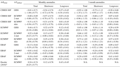
Table 1. The results of OLS regressions of1Rcloudagainst1Tsurface, with 95 % confidence interval over the March 2000 to June 2011 Terra
period. Values in parentheses use the unadjusted values of1CRF in the regressions. All estimates are in Wm−2K−1.
1Rclear 1Tsurface Monthly anomalies 3-month anomalies
Total Shortwave Longwave Total Shortwave Longwave CERES SSF GISS −0.81±0.71 −0.54±0.76 −0.27±0.45 −0.92±1.08 −0.72±1.12 −0.20±0.68 (−1.06±0.77) (−0.72±0.79) (−0.34±0.43) (−1.35±1.17) (−0.95±1.17) (−0.40±0.65) CERES SSF ECMWF −0.60±0.69 −0.57±0.74 −0.03±0.44 −0.54±1.05 −0.60±1.07 0.07±0.65 2-met (−0.88±0.75) (−0.78±0.77) (−0.10±0.42) (−0.96±1.15) (−0.86±1.12) (−0.10±0.63) CERES SSF ECMWF −0.31±0.71 −0.31±0.76 0.01±0.45 −0.20±1.08 −0.36±1.10 0.16±0.66 skin (−0.56±0.77) (−0.52±0.79) (−0.04±0.43) (−0.63±1.19) (−0.63±1.15) (0.00±0.64) ECMWF GISS 0.44±0.71 0.32±0.79 0.12±0.42 0.45±1.08 0.16±1.14 0.29±0.59 (0.18±0.80) (0.14±0.84) (0.05±0.42) (0.01±1.25) (−0.07±1.24) (0.08±0.60) ECMWF ECMWF 0.52±0.68 0.13±0.77 0.38±0.40 0.66±1.02 0.12±1.09 0.54±0.55 2-met (0.23±0.77) (−0.08±0.82) (0.31±0.40) (0.24±1.19) (−0.13±1.18) (0.37±0.56) ECMWF ECMWF 0.63±0.69 0.25±0.78 0.38±0.41 0.73±1.03 0.16±1.10 0.57±0.55 skin (0.38±0.79) (0.04±0.83) (0.34±0.41) (0.31±1.21) (−0.10±1.21) (0.41±0.56) EBAF GISS −0.13±0.64 −0.18±0.67 0.05±0.43 −0.20±0.99 −0.29±0.98 0.09±0.67 (−0.39±0.70) (−0.36±0.70) (−0.03±0.41) (−0.63±1.10) (−0.52±1.04) (−0.11±0.63) EBAF ECMWF −0.01±0.62 −0.24±0.65 0.23±0.42 0.08±0.94 −0.24±0.94 0.32±0.63 2-met (−0.29±0.68) (−0.45±0.68) (0.16±0.40) (−0.34±1.06) (−0.49±0.99) (0.15±0.60) EBAF ECMWF 0.18±0.63 −0.08±0.66 0.26±0.42 0.29±0.95 −0.12±0.96 0.41±0.63 skin (−0.08±0.70) (−0.29±0.69) (0.22±0.41) (−0.13±1.08) (−0.38±1.01) (0.25±0.60) Dessler ECMWF 0.54±0.74 0.12±0.78 0.43±0.45 N/A N/A N/A (2010)∗ (0.25±0.77)
∗Reported results from Dessler (2010) using ECMWF-CERES over the March 2000 through February 2010 period.
and−0.12 Wm−2K−1for GISS (Hansen et al., 2010), ERA-Interim 2-meter, and ERA-ERA-Interim skin temperatures, respec-tively. Also, as Dessler (2010) notes, the interannual changes in aerosol forcing affecting the all-sky CERES fluxes are not present in the modeled clear-sky fluxes, adding in another discrepancy. Although there is not necessarily a reason to be-lieve these aerosol effects would correlate with surface tem-perature anomalies, the low correlation between1Rcloudand 1Tsurface means that a few large discrepancies can have a
major impact on the estimate.
2.3 Surface temperature
For surface temperatures, global anomalies are calculated with respect to the two baseline periods (Terra and Aqua) discussed above. The temperatures sets used in the primary analysis are the GISS land-ocean temperature index (Hansen et al., 2010), ECMWF ERA-Interim 2-m air temperatures (t2m) for consistency with model-estimated feedbacks, and ECMWF ERA-Interim skin temperature (skt) for consistency with Dessler (2010). However, additional sensitivity tests are run using the global temperature anomalies from NCDC (Smith et al., 2008), HadCRUT3 (Brohan et al., 2006), and HadCRUT4 (Jones et al., 2012) (which is currently only available up to December 2010), as well as 2-m air tempera-tures from the MERRA and NCEP reanalysis products.
2.4 Removing non-cloud components from1CRF
The measured1CRF is influenced by other climate com-ponents besides clouds, due to the preferential TOA radia-tive effect these components have in clear-sky versus cloudy scenes. Generally, the positive surface albedo and water vapor feedbacks will bias towards a negative cloud feed-back if these effects are not removed, while the Planck re-sponse will create a bias in the opposite (positive) direc-tion, although the magnitude of the net bias is unclear. For comparison with Dessler (2010), we estimate the effect of these non-cloud components by combining the Geophysi-cal Fluid Dynamics Laboratory (GFDL) kernels (Soden et al., 2008) with ECMWF ERA-Interim reanalysis values, as well as the AIRS measured temperature and water vapor profiles where available (during the Aqua period). We also use 0.25 Wm−2to represent the change in well-mixed
green-house gas (WMGHG) forcing over this period, and 0.16 to represent the degree to which it preferentially affects the OLR in clear-sky vs. all-sky. This is applied by multiply-ing the factor by each month’s WMGHG forcmultiply-ing anomaly relative to the start of the period (linearly increasing), and subtracting the result from1CRF.
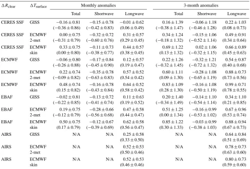
Table 2. The results of OLS regressions of1Rcloudagainst1Tsurface, with 95 % confidence interval over the September 2002 to June 2011
Aqua period. Values in parentheses use the unadjusted values of1CRF in the regressions. All estimates are in Wm−2K−1.
1Rclear 1Tsurface Monthly anomalies 3-month anomalies
Total Shortwave Longwave Total Shortwave Longwave CERES SSF GISS −0.16±0.81 −0.15±0.78 −0.01±0.62 0.16±1.39 −0.06±1.18 0.22±1.03 (−0.36±0.86) (−0.42±0.83) (0.06±0.49) (−0.38±1.47) (−0.46±1.28) (0.08±0.73) CERES SSF ECMWF 0.00±0.75 −0.32±0.72 0.31±0.57 0.34±1.24 −0.15±1.06 0.49±0.91 2-met (−0.31±0.79) (−0.60±0.76) (0.29±0.45) (−0.18±1.32) (−0.52±1.14) (0.34±0.64) CERES SSF ECMWF 0.33±0.75 −0.11±0.73 0.44±0.57 0.69±1.22 0.02±1.06 0.66±0.89 skin (0.00±0.80) (−0.38±0.77) (0.38±0.45) (0.13±1.32) (−0.32±1.15) (0.45±0.63) ECMWF GISS −0.06±0.80 −0.17±0.84 0.12±0.57 0.22±1.26 −0.32±1.21 0.54±0.87 (−0.26±0.88) (−0.45±0.90) (0.19±0.47) (−0.32±1.45) (−0.72±1.32) (0.40±0.68) ECMWF ECMWF 0.22±0.74 −0.35±0.78 0.57±0.52 0.60±1.11 −0.28±1.08 0.88±0.73 2-met (−0.09±0.82) (−0.63±0.83) (0.54±0.42) (0.09±1.30) (−0.65±1.19) (0.73±0.56) ECMWF ECMWF 0.48±0.74 −0.16±0.78 0.64±0.52 0.83±1.09 −0.16±1.08 0.99±0.71 skin (0.15±0.82) (−0.43±0.84) (0.58±0.42) (0.28±1.30) (−0.50±1.19) (0.78±0.55) EBAF GISS −0.02±0.81 −0.13±0.72 0.11±0.63 0.20±1.40 −0.14±1.10 0.34±1.10 (−0.22±0.85) (−0.41±0.74) (0.19±0.52) (−0.34±1.49) (−0.54±1.14) (0.21±0.85) EBAF ECMWF 0.19±0.75 −0.28±0.66 0.47±0.58 0.51±1.25 −0.16±0.99 0.67±0.96 2-met (−0.12±0.79) (−0.56±0.68) (0.44±0.47) (0.00±1.34) (−0.53±1.02) (0.53±0.74) EBAF ECMWF 0.50±0.75 −0.12±0.67 0.62±0.58 0.85±1.22 −0.03±0.99 0.88±0.94 skin (0.17±0.79) (−0.39±0.69) (0.56±0.47) (0.30±1.33) (−0.38±1.03) (0.67±0.73) AIRS GISS N/A N/A 0.25±0.58 N/A N/A 0.64±0.84 (0.33±0.50) (0.51±0.69) AIRS ECMWF N/A N/A 0.52±0.53 N/A N/A 0.78±0.73
2-met (0.50±0.46) (0.63±0.60)
AIRS ECMWF N/A N/A 0.52±0.53 N/A N/A 0.80±0.73
skin (0.46±0.46) (0.59±0.60)
For an estimate of the potential bias, we compare the es-timated cloud feedback using the ERA-Interim reanaly-sis OLR adjustments vs. AIRS OLR adjustments over the overlapping Aqua period (Fig. 3). The difference (ERA-adjustedRcloud minus AIRS-adjustedRcloud) is 0.17, 0.07,
and 0.04 Wm−2K−1for GISS, Interim 2-m, and ERA-Interim skin temperature, respectively. As AIRS is not avail-able for the SW component or during the beginning of the Terra period, it is not used for those adjustments and ERA-Interim is used instead (Tables 1 and 2).
Another potential issue is that, since GCMs generally do a poor job of reproducing the vertical distribution of clouds (Zhang et al., 2005), the all-sky kernels calculated from such a model may not accurately represent the real-world effect of these non-cloud components on the TOA radiation bud-get. Additionally, aerosol changes may also produce a non-cloud influence on1CRF, whether they result from small volcanic eruptions (Solomon et al., 2011) or are of anthro-pogenic origin (Kaufmann et al., 2011), although signifi-cant influence on the apparent cloud feedback is question-able, because, as discussed previously, these aerosol varia-tions are not expected to correlate with the monthly surface
26 1
Figure 3. Global monthly anomalies for the cloud radiative forcing from CERES SSF without 2
adjustments (ΔCRF), and with adjustments using ECMWF (ΔRcloud,ECMWF-adj) or AIRS
3
(ΔRcloud,AIRS-adj) for water vapor, temperature, and WMGHG contributions. Both versions of
4
ΔRcloud use ECMWF albedo for adjustments.
5
6
Fig. 3. Global monthly anomalies for the cloud radiative
forcing from CERES SSF without adjustments (1CRF), and with adjustments using ECMWF (1Rcloud,ECMWF-adj) or AIRS
(1Rcloud,AIRS-adj) for water vapor, temperature, and WMGHG
contributions. Both versions of1Rcloud use ECMWF albedo for
adjustments.
temperature variations. Nonetheless, for these reasons we also present our regressions of the unadjusted1CRF against surface temperature (Tables 1 and 2).
3 Results
Tables 1 and 2 show the results of the OLS (ordinary least squares) regressions, with uncertainties presented for the 2.5 % to 97.5 % confidence interval as a result of those regressions (no explicit uncertainty calculations have been made for uncertainty in forcings or measurements). Ther2 values for these 1Rcloud versus 1Tsurface regressions
us-ing monthly anomalies and CERES-only derived 1CRF during the Terra period are 3.7 %, 2.1 %, and 0.5 % for GISS, ECMWF 2-m and skin temperatures, respectively, with 1.1 %, 1.6 %, and 2.4 % for CERES-ECMWF using the same temperature sets. It is during this time period that the larger sensitivity to clear-sky flux data exists, with the CERES SSF estimate generally suggesting a modest to large negative cloud feedback, whereas the CERES-ECMWF esti-mate implies a modest positive cloud feedback, with CERES-EBAF falling in the middle. Table 3 shows that the sensitiv-ity to clear-sky flux source extends even to the reanalyses products, with the difference between MERRA and ERA-Interim estimates ranging from 0.45 to −0.04 Wm−2K−1, and MERRA generally producing the more positive estimate of the cloud feedback.
The sensitivity of these regressions to the start date can be seen in Fig. 4. During the Aqua period, there is better agree-ment among the ECMWF, CERES (both SSF and EBAF), and AIRS modeled clear sky estimates, with either a slightly negative or positive net cloud feedback implied, but this pe-riod shows a large sensitivity to the choice of temperature dataset. Table 4 highlights this sensitivity with seven dif-ferent temperature datasets. Using MERRA or HadCRUT3 temperatures produces very large positive estimates for the cloud feedback, although the newer HadCRUT4 results in more negative estimates better in line with GISS and NCEP. There is less sensitivity of the sign over this period for the separate shortwave and longwave components, with most re-sults showing a negative shortwave feedback and a positive longwave feedback, although again using the MERRA re-analysis produces an exception.
The effect of the kernel adjustments can also be seen in these tables. According to the AIRS observations used for these adjustments over the Aqua period, the net combination of the water vapor, Planck, and WMGHG components leads only to tiny negative or even positive bias in the unadjusted 1CRF regressions. This is different from the long-term ef-fect of these non-cloud components in models, which cre-ate a larger negative bias in the unadjusted1CRF, but likely results here from the better month-to-month correlation be-tween the Planck response and1Tsurfacethan between water
vapor anomalies and1Tsurface.
27 1
Figure 4. The sensitivity of
dT dCRF
to different start dates (all regressions end in 6/2011), 2
showing all regressions four years or longer. GISS is used for ΔTsurface.
3
Fig. 4. The sensitivity ofdCRFdT to different start dates (all regressions end in June 2011), showing all regressions four years or longer. GISS is used for1Tsurface.
The results also suggest that there is not much to be gained by using seasonal rather than monthly anomalies in this anal-ysis, as the uncertainty bounds only increase due to the fewer available observations, while failing to illuminate a strong signal absent in the monthly anomalies.
4 Discussion
Overall, the results show that estimates for the net short-term feedback using this methodology are sensitive to tempera-ture datasets, the time period for which we run the regres-sions, and the choice of clear-sky radiation fluxes. The large uncertainties and sensitivities make it difficult to deem the GCM positive cloud feedbacks inconsistent with observa-tions. Similarly, the uncertainty makes it difficult to rule out the possibility of a large negative cloud feedback. However, over the Aqua period, the majority of datasets point to a neg-ative feedback in the SW component, in contrast to a positive feedback in the LW component. These results tend to be op-posite of those found in Zelinka and Hartmann (2011), who examined only the tropical means and found a negative LW feedback counteracted by a positive SW cloud feedback, with a net positive feedback. Davies and Molloy (2012) used a dif-ferent method, examining the 10-yr negative trend in cloud height as retrieved from the Multiangle Imaging SpectroRa-diometer (MISR) aboard Terra, in order to infer a potential negative LW cloud feedback.
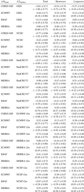
Table 3. Extended sensitivity tests. As in Table 1, but with additional temperature and clear-sky flux datasets, and only using monthly
anomalies.
1Rclear 1Tsurface Total Shortwave Longwave
CERES SSF GISS −0.81±0.71 −0.54±0.76 −0.27±0.45 (−1.06±0.77) (−0.72±0.79) (−0.34±0.43)
ECMWF GISS 0.44±0.71 0.32±0.79 0.12±0.42
(0.18±0.80) (0.14±0.84) (0.05±0.42)
EBAF GISS −0.13±0.64 −0.18±0.67 0.05±0.43
(−0.39±0.70) (−0.36±0.70) (−0.03±0.41)
MERRA GISS 0.86±0.70 0.48±0.71 0.38±0.42
(0.60±0.77) (0.30±0.74) (0.30±0.41) CERES SSF NCDC −0.77±0.86 −0.62±0.92 −0.16±0.54 (−1.02±0.93) (−0.78±0.96) (−0.24±0.53)
ECMWF NCDC 0.43±0.85 0.39±0.95 0.04±0.50
(0.18±0.96) (0.23±1.01) (−0.05±0.50)
EBAF NCDC −0.12±0.77 −0.31±0.81 0.19±0.52
(−0.37±0.85) (−0.47±0.84) (0.10±0.50)
MERRA NCDC 0.79±0.85 0.44±0.85 0.35±0.50
(0.54±0.94) (0.28±0.90) (0.26±0.50) CERES SSF HadCRUT3 −0.27±0.93 −0.42±0.99 0.15±0.58 (−0.69±1.01) (−0.66±1.02) (−0.03±0.56)
ECMWF HadCRUT3 0.54±0.91 0.25±1.02 0.30±0.53
(0.13±1.03) (0.01±1.08) (0.12±0.53)
EBAF HadCRUT3 0.33±0.82 −0.23±0.86 0.56±0.55
(−0.09±0.91) (−0.47±0.90) (0.38±0.53)
MERRA HadCRUT3 0.98±0.90 0.47±0.91 0.51±0.54
(0.56±1.00) (0.23±0.96) (0.33±0.53) CERES SSF HadCRUT4∗ −0.96±0.81 −0.71±0.89 −0.25±0.51
(−1.25±0.88) (−0.93±0.92) (−0.32±0.50) ECMWF HadCRUT4∗ 0.54±0.84 0.37±0.93 0.17±0.48 (0.25±0.95) (0.14±0.98) (0.11±0.49) EBAF HadCRUT4∗ −0.10±0.74 −0.21±0.78 0.10±0.48 (−0.39±0.82) (−0.43±0.82) (0.04±0.47) MERRA HadCRUT4∗ 0.99±0.84 0.50±0.84 0.49±0.48
(0.70±0.93) (0.27±0.88) (0.42±0.48) CERES SSF ECMWF t2m −0.60±0.69 −0.57±0.74 −0.03±0.44 (−0.88±0.75) (−0.78±0.77) (−0.10±0.42)
ECMWF ECMWF t2m 0.52±0.68 0.13±0.77 0.38±0.40
(0.23±0.77) (−0.08±0.82) (0.31±0.40) EBAF ECMWF t2m −0.01±0.62 −0.24±0.65 0.23±0.42 (−0.29±0.68) (−0.45±0.68) (0.16±0.40)
MERRA ECMWF t2m 0.72±0.68 0.25±0.69 0.47±0.40
(0.44±0.75) (0.04±0.72) (0.40±0.40) CERES SSF MERRA t2m 0.00±0.74 −0.16±0.78 0.16±0.46 (−0.20±0.80) (−0.29±0.82) (0.08±0.45)
ECMWF MERRA t2m 0.65±0.72 0.48±0.80 0.17±0.42
(0.45±0.81) (0.35±0.85) (0.10±0.42) EBAF MERRA t2m 0.41±0.65 −0.08±0.69 0.49±0.43 (0.20±0.72) (−0.21±0.72) (0.42±0.42)
MERRA MERRA t2m 0.62±0.72 0.36±0.72 0.25±0.43
(0.41±0.79) (0.23±0.76) (0.18±0.42) CERES SSF NCEP t2m −0.77±0.61 −0.56±0.65 −0.21±0.39 (−0.97±0.65) (−0.68±0.68) (−0.30±0.37)
ECMWF NCEP t2m 0.59±0.60 0.38±0.67 0.21±0.35
(0.39±0.68) (0.26±0.72) (0.13±0.36) EBAF NCEP t2m −0.07±0.55 −0.17±0.58 0.10±0.37 (−0.28±0.60) (−0.29±0.60) (0.01±0.35)
MERRA NCEP t2m 0.93±0.59 0.39±0.61 0.54±0.35
(0.73±0.66) (0.28±0.64) (0.45±0.35)
∗HadCRUT4 is only available up to December 2010.
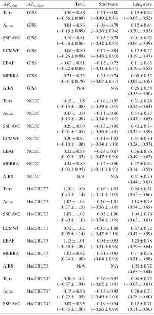
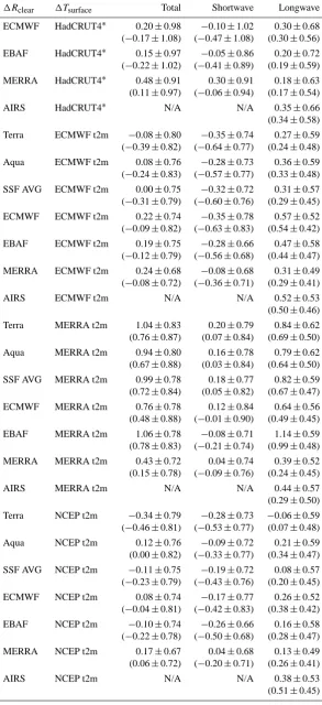
Table 4. Extended sensitivity tests. As in Table 2, but with additional temperature and clear-sky flux datasets, and only using monthly
anomalies.
1Rclear 1Tsurface Total Shortwave Longwave
Table 4. Continued.
1Rclear 1Tsurface Total Shortwave Longwave
ECMWF HadCRUT4∗ 0.20±0.98 −0.10±1.02 0.30±0.68 (−0.17±1.08) (−0.47±1.08) (0.30±0.56) EBAF HadCRUT4∗ 0.15±0.97 −0.05±0.86 0.20±0.72 (−0.22±1.02) (−0.41±0.89) (0.19±0.59) MERRA HadCRUT4∗ 0.48±0.91 0.30±0.91 0.18±0.63 (0.11±0.97) (−0.06±0.94) (0.17±0.54) AIRS HadCRUT4∗ N/A N/A 0.35±0.66 (0.34±0.58) Terra ECMWF t2m −0.08±0.80 −0.35±0.74 0.27±0.59 (−0.39±0.82) (−0.64±0.77) (0.24±0.48) Aqua ECMWF t2m 0.08±0.76 −0.28±0.73 0.36±0.59 (−0.24±0.83) (−0.57±0.77) (0.33±0.48) SSF AVG ECMWF t2m 0.00±0.75 −0.32±0.72 0.31±0.57 (−0.31±0.79) (−0.60±0.76) (0.29±0.45) ECMWF ECMWF t2m 0.22±0.74 −0.35±0.78 0.57±0.52 (−0.09±0.82) (−0.63±0.83) (0.54±0.42) EBAF ECMWF t2m 0.19±0.75 −0.28±0.66 0.47±0.58 (−0.12±0.79) (−0.56±0.68) (0.44±0.47) MERRA ECMWF t2m 0.24±0.68 −0.08±0.68 0.31±0.49 (−0.08±0.72) (−0.36±0.71) (0.29±0.41) AIRS ECMWF t2m N/A N/A 0.52±0.53 (0.50±0.46) Terra MERRA t2m 1.04±0.83 0.20±0.79 0.84±0.62 (0.76±0.87) (0.07±0.84) (0.69±0.50) Aqua MERRA t2m 0.94±0.80 0.16±0.78 0.79±0.62 (0.67±0.88) (0.03±0.84) (0.64±0.50) SSF AVG MERRA t2m 0.99±0.78 0.18±0.77 0.82±0.59 (0.72±0.84) (0.05±0.82) (0.67±0.47) ECMWF MERRA t2m 0.76±0.78 0.12±0.84 0.64±0.56 (0.48±0.88) (−0.01±0.90) (0.49±0.45) EBAF MERRA t2m 1.06±0.78 −0.08±0.71 1.14±0.59 (0.78±0.83) (−0.21±0.74) (0.99±0.48) MERRA MERRA t2m 0.43±0.72 0.04±0.74 0.39±0.52 (0.15±0.78) (−0.09±0.76) (0.24±0.45) AIRS MERRA t2m N/A N/A 0.44±0.57 (0.29±0.50) Terra NCEP t2m −0.34±0.79 −0.28±0.73 −0.06±0.59 (−0.46±0.81) (−0.53±0.77) (0.07±0.48) Aqua NCEP t2m 0.12±0.76 −0.09±0.72 0.21±0.59 (0.00±0.82) (−0.33±0.77) (0.34±0.47) SSF AVG NCEP t2m −0.11±0.75 −0.19±0.72 0.08±0.57 (−0.23±0.79) (−0.43±0.76) (0.20±0.45) ECMWF NCEP t2m 0.08±0.74 −0.17±0.77 0.26±0.52 (−0.04±0.81) (−0.42±0.83) (0.38±0.42) EBAF NCEP t2m −0.10±0.74 −0.26±0.66 0.16±0.58 (−0.22±0.78) (−0.50±0.68) (0.28±0.47) MERRA NCEP t2m 0.17±0.67 0.04±0.68 0.13±0.49 (0.06±0.72) (−0.20±0.71) (0.26±0.41) AIRS NCEP t2m N/A N/A 0.38±0.53 (0.51±0.45)
∗HadCRUT4 is only available up to December 2010.
time of the noise (Spencer and Braswell, 2008), this could lead to a positive bias in the diagnosed cloud feedback. This is because the cloud radiative effects, which may even orig-inate in response to (for example) changing ocean tempera-tures in another region, would necessarily influence surface temperatures, but this method would always incorrectly clas-sify the increased (decreased) downward radiation as a posi-tive feedback to increasing (decreasing) temperatures in that region, rather than the cause. Of course, this bias only exists if the temperature response is correlated with the radiative effects, which in turn means the response must come within the decorrelation time of such effects. An attempt has been made to show that these fluctuations in the cloud forcing are insignificant relative to the variability in ocean heat exchange between layers, noting that the standard deviation of ocean heat flux from ARGO measurements down to the 700 m layer would correspond to a monthly forcing of 13 Wm−2 and a
ratio ofσ (1Focean)/σ (1Rcloud)≈20 (Dessler, 2011).
Esti-mating the heat flux of a more realistic 100 m mixed layer from ocean temperature anomalies (Levitus et al., 2009), however, results in a standard deviation of 2.1 Wm−2for 3-month averages. Obviously, using a singular depth to repre-sent the mixed layer is problematic due to the spatial and sea-sonal heterogeneity. Nonetheless, a lower value for mixed-layer heat capacity on these times scales is more in line with recent regressions, which have found that the relatively small variations associated with the solar cycle (∼0.25 Wm−2) can be detected in global surface temperatures, with an instanta-neous response of ∼0.4 K/(Wm−2) after only a month lag (Foster and Rahmstorf, 2011). If a similar efficacy were to exist for radiative noise due to cloud variations, this noise could significantly contaminate the cloud feedback estimate. The extent of this contamination thus depends on the amount non-feedback radiative variability, as well as the decorrela-tion time of the radiative noise produced.
Finally, Dessler (2010) notes that there is no correlation between the short- and long-term cloud feedbacks among models, so that the long-term feedback may be significantly higher or lower than that diagnosed from interannual vari-ations. This fact, combined with the sensitivity of the esti-mated short-term feedback to methodological choices, sug-gests that diagnosing a climate-scale cloud feedback in this manner will require a substantially longer time period.
Supplementary material related to this article is available online at: http://www.earth-syst-dynam.net/3/ 97/2012/esd-3-97-2012-supplement.zip.
Acknowledgements. We thank the CERES team, and N. G. Loeb
in particular for information regarding the datasets. We thank A. E. Dessler for guidance in reproducing his results, and Alexan-dra Jonko of Oregon State for her help in utilizing the radiative kernels. The reviewers of the manuscript provided numerous constructive comments in helping improve the paper. The AIRS
data product was provided by the NASA Goddard Earth Sciences Data and Information Services Center (DISC). ECMWF ERA-Interim data used in this study have been obtained from the ECMWF Data Server. NCEP Reanalysis data were retrieved from the NOAA Earth System Research Library Physical Sciences Division website at http://www.esrl.noaa.gov/. Global MERRA data used in this study were produced with the Giovanni online data system, developed and maintained by the NASA GES DISC at http://disc.sci.gsfc.nasa.gov/giovanni/.
Edited by: J. C. Hargreaves
References
Allan, R. P.: Combining satellite data and models to estimate cloud radiative effect at the surface and in the atmosphere, Meteorol. Appl., 18, 324–333, doi:10.1002/met.285, 2011.
Allan, R. P., Ringer, M. A., and Slingo, A.: Evaluation of moisture in the Hadley Centre Climate Model using simulations of HIRS water vapour channel radiances, Q. J. Roy. Meteorol. Soc., 129, 3371-3389, doi:10.1256/qj.02.217, 2003.
Andrews, T., Forster, P. M., Boucher, O., Bellouin, N., and Jones, A.: Precipitation, radiative forcing and global temperature change, Geophys. Res. Lett., 37, L14701, doi:10.1029/2010GL043991, 2010.
Bender, F. A.-M.: Planetary albedo in strongly forced climate, as simulated by the CMIP3 models, Theor. Appl. Climatol., 105, 529–535, doi:10.1007/s00704-011-0411-2, 2011.
Bony, S. R., Colman, R., Kattsov, V. M., Allan, R. P., Brether-ton, C. S., Dufresne, J.-J., Hall, A., Hallegatte, S., Holland, M. M., Ingram, W., Randall, D. A., Soden, B. J., Tselioudis, G., and Webb, M. J.: How well do we understand and evaluate cli-mate change feedback processes?, J. Clicli-mate, 19, 3445–3482, doi:10.1175/JCLI3819.1, 2006.
Brohan, P., Kennedy, J. J., Harris, I., Tett, S. F. B., and Jones, P. D.: Uncertainty estimates in regional and global observed tempera-ture changes: A new dataset from 1850, J. Geophys. Res., 111, D12106, doi:10.1029/2005JD006548, 2006.
Cess, R. D. and Potter, G. L.: Exploratory studies of cloud radiative forcing with a general circulation model, Tellus, 39, 460–473, 1987.
Chahine, M. T., Pagano, T. S., Aumann, H. H., Atlas, R., Barnet, C., Blaisdell, J., Chen, L., Divakarla, M., Fetzer, E., Goldberg, M., Gautier, C., Granger, S., Hannon, S., Irion, F. W., Kakar, R., Kalnay, E., Lambrigtsen, B. H., Lee, S.-Y., Marshall, J. L., McMillan, W. W., McMillin, L., Olsen, E. T., Revercomb, H., Rosenkranz, P., Smith, W. L., Staelin, D., Strow, L. L., Susskind, J., Tobin, D., Wolf, W., and Zhou, L.: AIRS: Improving Weather Forecasting and Providing New Data on Greenhouse Gases, B. Am. Meteorol. Soc., 87, 911–926, 2006.
Davies, R. and Molloy, M.: Global cloud height fluctuations mea-sured by MISR on Terra from 2000 to 2010, Geophys. Res. Lett., 39, L03701, doi:10.1029/2011GL050506, 2012.
McNally, A. P., Monge-Sanz, B. M., Morcrette, J.-J., Park, B.-K., Peubey, C., de Rosnay, P., Tavolato, C., Th´epaut, J.-N., and Vitart, F.: The ERA-interim reanalysis: configuration and perfor-mance of the data assimilation system, data available at: http:// data-portal.ecmwf.int/data/d/interimmoda/levtype=sfc/, last ac-cess: 4 January 2012, Q. J. Roy. Meteorol. Soc., 137, 553–597, doi:10.1002/qj.828, 2011.
Dessler, A. E.: A determination of the cloud feedback from cli-mate variations over the past decade, Science, 330, 1523–1527, doi:10.1126/science.1192546, 2010.
Dessler, A. E.: Cloud variations and the Earth’s energy budget, Geo-phys. Res. Lett., 38, L19701, doi:10.1029/2011GL049236, 2011. Erlick, C. and Ramaswamy, V.: Note on the de?nition of clear sky in calculations of short wave cloud forcing, J. Geophys. Res., 108, 4156, doi:10.1029/2002JD002990, 2003.
Foster, G. and Rahmstorf, S.: Global temperature evolution 1979–2010, Environ. Res. Lett., 6, 044022, doi:10.1088/1748-9326/6/4/044022, 2011.
Hansen, J., Ruedy, R., Sato, M., and Lo, K.: Global sur-face temperature change, Rev. Geophys., 48, RG4004, doi:10.1029/2010RG000345, 2010.
John, V. O., Allan, R. P., and Soden, B. J.:, How robust are observed and simulated precipitation responses to trop-ical ocean warming?, Geophys. Res. Lett., 36, L14702, doi:10.1029/2009GL038276, 2009.
Jones, P. D., Lister, D. H., Osborn, T. J., Harpham, C., Salmon, M., and Morice, C. P.: Hemispheric and large-scale land-surface air temperature variations: An extensive revi-sion and an update to 2010, J. Geophys. Res., 117, D05127, doi:10.1029/2011JD017139, 2012.
Kaufmann, R. K., Kauppi, H., Mann, M. L., and Stock, J. H.: Reconciling anthropogenic climate change with observed tem-perature 1998–2008, P. Natl. Acad. Sci., 108, 11790–11793, doi:10.1073/pnas.1102467108, 2011.
Lee, J., Yang, P., Dessler, A. E., Gao, B.-C., and Platnick, S.: Distri-bution and Radiative Forcing of Tropical Thin Cirrus Clouds, J. Atmos. Sci., 66, 3721–3731, doi:10.1175/2009JAS3183.1, 2009. Levitus, S., Antonov, J. I., Boyer, T. P., Locarnini, R. A., Garcia, H. E., and Mishonov, A. V.: Global ocean heat content 1995– 2008 in light of recently revealed instrumentation problems, data available from: http://www.nodc.noaa.gov/OC5/3M HEAT CONTENT/anomaly data.html, last access: 14 September 2011, Geophys. Res. Lett., 36, L07608, doi:10.1029/2008GL037155, 2009.
Loeb, N. G., Wielicki, B. A., Doelling, D. R. , Smith, G. L., Keyes, D. F., Kato, S., Manlo-Smith, N., and Wong, T.: Toward Optimal Closure of the Earth’s TOA Radiation Budget, J. Climate, 22, 748–766, doi:10.1175/2008JCLI2637.1, 2009.
Loeb, N. G., Kato, S., Su, W., Wong, T., Rose, F. G., Doelling, D. R., Norris, J. R., and Huang, X.: Advances in Understanding Top-of-Atmosphere Radiation Variability from Satellite Observations, Surv. Geophys., 33, 359–385, doi:10.1007/s10712-012-9175-1, 2012.
Rienecker, M. M., Suarez, M. J., Gelaro, R., Todling, R., Bacmeis-ter, J., Liu, E., Bosilovich, M. G., Schubert, S. D., Takacs, L., Kim, G.-K., Bloom, S., Chen, J., Collins, D., Conaty, A., da Silva, A., Gu, W., Joiner, J., Koster, R. D., Lucchesi, R., Molod, A., Owens, T., Pawson, S., Pegion, P., Redder, C. R., Reichle, R., Robertson, F. R., Ruddick, A. G., Sienkiewicz, M.,
and Woollen, J.: MERRA – NASA’s Modern-Era Retrospective Analysis for Research and Applications, J. Climate, 24, 3624– 3648, doi:10.1175/JCLI-D-11-00015.1, 2011.
Shell, K. M., Kiehl, J. T., and Shields, C. A.: Using the radia-tive kernel technique to calculate climate feedbacks in NCAR’s Community Atmospheric Model, J. Climate, 21, 2269–2282, doi:10.1175/2007JCLI2044.1, 2008.
Smith, T. M., Reynolds, R. W., Peterson, T. C., and Lawrimore, J.: Improvements to NOAA’s Historical Merged Land-Ocean Surface Temperature Analysis (1880–2006), data available at: ftp://ftp.ncdc.noaa.gov/pub/data/anomalies/monthly.land ocean. 90S.90N.df 1901-2000mean.dat, last access: 4 January 2012, J. Climate, 21, 2283–2293, doi:10.1175/2007JCLI2100.1, 2008. Soden, B. J., Held, I. M., Colman, R., Shell, K. M., Kiehl, J. T., and
Shields, C. A: Quantifying climate feedbacks using radiative ker-nels, J. Climate, 21, 3504–3520, doi:10.1175/2007JCLI2110.1, 2008.
Sohn, B.-J. and Bennartz, R.: Contribution of water vapor to obser-vational estimates of longwave cloud radiative forcing, J. Geo-phys. Res., 113, D20107, doi:10.1029/2008JD010053, 2008. Solomon, S., Daniel, J. S., Neely III, R. R., Vernier, J. P.,
Dut-ton, E. G., and Thomason, L. W.: The Persistently Variable “Background” Stratospheric Aerosol Layer and Global Climate Change, Science, 333, 866–870, doi:10.1126/science.1206027, 2011.
Spencer, R. W. and Braswell, W. D.: Potential biases in feedback di-agnosis from observational data: A simple model demonstration, J. Climate, 21, 5624–5628, doi:10.1175/2008JCLI2253.1, 2008. Spencer, R. W., Braswell, W. D., Christy, J. R., and Hnilo, J.: Cloud and radiation budget changes associated with tropical intraseasonal oscillations, Geophys. Res. Lett., 34, L15707, doi:10.1029/2007GL029698, 2007.
Sun, W., Lin, B., Hu, Y., Lukashin, C., Kato, S., and Liu, Z.: On the consistency of CERES longwave flux and AIRS tem-perature and humidity profiles, J. Geophys. Res., 116, D17101, doi:10.1029/2011JD016153, 2011.
Wielicki, B. A., Barkstrom, B. R., Baum, B. A., Charlock, T. P., Green, R. N., Kratz, D. P, Lee, R. B., Minnis, P., Smith, G. L., Wong, T., Young, D. F., Cess, R. D., Coakley, J. A., Cromme-lynck, A. D., Donner, L., Kandel, R., King, M. D., Miller, A. J., Ramanathan, V., Randall, D. A., Stowe, L. L., and Welch, R. M.: Clouds and the Earth’s Radiant Energy System (CERES): Algorithm overview, data available at: http://ceres.larc.nasa.gov/ order data.php, last access: 12 January 2012, IEEE T. Geosci. Remote, 36, 1127–1141, doi:10.1109/36.701020, 1998. Zelinka, M. D. and Hartmann, D. L.: The observed sensitivity of
high clouds to mean surface temperature anomalies in the trop-ics, J. Geophys. Res., 116, D23103, doi:10.1029/2011JD016459, 2011.
Zhang, M. H., Lin, W. Y., Klein, S. A., Bacmeister, J. T., Bony, S., Cederwall, R. T., Del Genio, A. D., Hack, J. J., Loeb, N. G., Lohmann, U., Minnis, P., Musat, I., Pincus, R., Stier, P., Suarez, M. J., Webb, M. J., and Wu, J. B.: Comparing clouds and their seasonal variations in 10 atmospheric general circulation mod-els with satellite measurements, J. Geophys. Res., 110, D15S02, doi:10.1029/2004JD005021, 2005.