Improved methods for signal processing in measurements of
mercury by Tekran
®
2537A and 2537B instruments
Jesse L. Ambrose
College of Engineering and Physical Sciences, University of New Hampshire, Durham, 03824, USA
Correspondence:Jesse L. Ambrose ([email protected])
Received: 27 April 2017 – Discussion started: 15 August 2017
Revised: 27 October 2017 – Accepted: 6 November 2017 – Published: 22 December 2017
Abstract. Atmospheric Hg measurements are commonly
carried out using Tekran®Instruments Corporation’s model 2537 Hg vapor analyzers, which employ gold amalgamation preconcentration sampling and detection by thermal desorp-tion (TD) and atomic fluorescence spectrometry (AFS). A generally overlooked and poorly characterized source of an-alytical uncertainty in those measurements is the method by which the raw Hg atomic fluorescence (AF) signal is cessed. Here I describe new software-based methods for pro-cessing the raw signal from the Tekran® 2537 instruments, and I evaluate the performances of those methods together with the standard Tekran®internal signal processing method. For test datasets from two Tekran®instruments (one 2537A and one 2537B), I estimate that signal processing uncertain-ties in Hg loadings determined with the Tekran®method are within±[1 %+ 1.2 pg] and±[6 %+0.21 pg], respectively. I demonstrate that the Tekran®method can produce signif-icant low biases (≥5 %) not only at low Hg sample load-ings (<5 pg) but also at tropospheric background concentra-tions of gaseous elemental mercury (GEM) and total mercury (THg) (∼1 to 2 ng m−3)under typical operating conditions (sample loadings of 5–10 pg). Signal processing uncertain-ties associated with the Tekran®method can therefore rep-resent a significant unaccounted for addition to the overall ∼10 to 15 % uncertainty previously estimated for Tekran® -based GEM and THg measurements. Signal processing bias can also add significantly to uncertainties in Tekran®-based gaseous oxidized mercury (GOM) and particle-bound mer-cury (PBM) measurements, which often derive from Hg sam-ple loadings<5 pg. In comparison, estimated signal process-ing uncertainties associated with the new methods described herein are low, ranging from within ±0.053 pg, when the Hg thermal desorption peaks are defined manually, to within
±[2 %+0.080 pg] when peak definition is automated. Mer-cury limits of detection (LODs) decrease by 31 to 88 % when the new methods are used in place of the Tekran®method. I recommend that signal processing uncertainties be quantified in future applications of the Tekran®2537 instruments.
1 Introduction
Gold amalgamation preconcentration, followed by thermal desorption (TD) in Ar carrier gas and detection via atomic fluorescence spectrometry (AFS), is a commonly used method for quantifying atmospheric elemental mercury va-por, Hg0(g) (hereafter referred to as gaseous elemental mer-cury, GEM) (Schroeder et al., 1995; Gustin and Jaffe, 2010; Pandy et al., 2011). Coupled with various sample capture and pretreatment methods, the above measurement scheme is also used for quantitative analysis of atmospheric gaseous oxidized mercury (GOM) (Stratton and Lindberg, 1995; Lan-dis et al., 2002; Lyman et al., 2007), total gaseous mercury (TGM≡GEM+GOM) (Ambrose et al., 2015), atmospheric particle-bound mercury (PBM) (Landis et al., 2002), atmo-spheric total mercury (THg≡GEM+GOM+PBM) (Jaffe et al., 2005), and total aqueous Hg (USEPA, 2002). Most AFS-based atmospheric Hg measurements employ Tekran® Instruments Corporation’s model 2537 Hg vapor analyzers (versions A and B; hereafter referred to collectively as “the Tekran® analyzer”) (Schroeder et al., 1995; Landis et al., 2002; Tekran Corporation, 2006, 2007).
uncertainty is the method by which the raw Hg atomic fluo-rescence (AF) signal is processed by the Tekran®analyzer. Although most researchers rely on the Tekran® analyzer’s embedded software to automatically integrate the Hg TD peaks, Swartzendruber et al. (2009) and Slemr et al. (2016) demonstrated that the accuracy and precision of the Tekran® peak integration method can significantly decline at low Hg loadings.
To better characterize the analytical uncertainty associated with atmospheric Hg measurements made with the Tekran® analyzer, and in an attempt to improve upon existing mea-surement methods for atmospheric Hg, I developed new software-based methods for offline processing of the raw Hg AF signal from the Tekran®analyzer. Here I describe the key features of the new signal processing methods and charac-terize their performances, together with that of the standard Tekran®signal processing method.
2 Experimental
Using National Instruments™ LabVIEW software (version 12.0), I developed a virtual instrument (VI) for offline pro-cessing of the serial data output from Tekran®models 2537A and 2537B mercury vapor analyzers. The VI is character-ized and validated using data collected as part of the Nitro-gen, Oxidants, Mercury, and Aerosol Distributions, Sources, and Sinks (NOMADSS) campaign (https://www.eol.ucar. edu/field_projects/nomadss) using a Tekran® 2537A instru-ment and a 2537B instruinstru-ment incorporated in the Univer-sity of Washington’s Detector for Oxidized Hg Species (Ly-man and Jaffe, 2012; Ambrose et al., 2013, 2015; Am-brose, 2017). The instrument configurations are described in Ambrose et al. (2015). Instrument operating parameters are given in Table S1 in the Supplement. The most signif-icant difference between the two instruments tested is that the 2537B instrument was modified to improve its signal-to-noise ratio. The instrument’s sample cuvette and detector bandpass filter were replaced with a mirrored cuvette and an improved bandpass filter, respectively (Ambrose et al., 2013). The cuvette and bandpass filter were obtained from Tekran® (part numbers 40-25105-00 and 40-25200-02, re-spectively).
All linear regression equations reported herein were cal-culated by the bisquare method (unweighted) in LabVIEW. All stated uncertainties represent 95 % confidence intervals, unless otherwise specified.
Virtual instrument design overview
2.1 Operation
The VI’s Hg atomic fluorescence signal processing method parses the Tekran® analyzer’s serial data output (RAW-DUMP format; see Sect. S1 in the Supplement) using text
delimiters associated with each component (Figs. S1 and S2 in the Supplement).
At the start of an analysis, the VI computes the overall mean baseline standard deviation,σbl, for all samples in the
data file to be analyzed. The baseline standard deviation for each sample is first calculated as the 10-point (1 s) running mean of the baseline measurements made from 1 s after the start of the AF signal recording interval to 2 s prior to the ap-proximate start of the Au trap desorption cycle (i.e., the value of the “BL time” parameter in Table S1 in the Supplement). The value ofσbl is then calculated from the values for all
individual samples.
For each sample analysis cycle, the VI carries out the fol-lowing operations:
1. The “raw data” string (Fig. S1) is converted to an array of 10 Hz AF signal values.
2. The timestamp, cycle-type flag, and trap identity are ex-tracted from the “final data” string (Fig. S1).
3. Anx–yplot is generated from the data array created in step 1.
4. Unless the VI is set to automatically define the Hg ther-mal desorption peaks, the user is prompted to identify the start time,tstart, of the TD peak. This selection is
ac-complished by first manually setting the placement of a cursor on thex–y plot generated in step 3 and then using a control to extract the associated coordinates. Alternatively, values oftstart can be set to values
de-fined automatically during the initialization procedure (see below). The mean baseline voltage at the start of the TD peak is calculated over the interval fromtstartto tstart−9 ds (n=10 data points).
5. The coordinates of the Hg TD peak maximum are iden-tified automatically from the data array created in step 1. In my experience, the Tekran® analyzer’s baseline generally decreases (slopes downward) across the Hg TD peak. I parameterized the VI for such a condition by identifying the TD peak maximum as the largest AF signal value recorded aftertstart.
6. A preliminary TD peak height value is calculated from the mean baseline voltage at the start of the peak (step 4) and the maximum voltage (step 5). In cases when the preliminary peak height is a negative number, the VI sets the value toσbl. (See Sect. S3 for further details.)
7. Based on user-defined settings on the VI’s front panel, the TD peak end coordinates are either selected manu-ally (as for the peak start time in step 4) or calculated automatically from the peak maximum in step 5 and the initialization parameters (as described below).
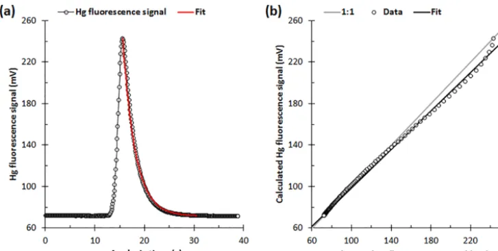
Figure 1. (a)Example Hg thermal desorption profile during a calibration gas analysis cycle on a Tekran®2537A instrument. Also shown is the corresponding 150-point exponential bisquare (unweighted) regression fit (Eq. 1;r2=0.998) used to derive the decay constant (b= −0.041±0.004 ds−1)during initialization of the VI’s signal processing method.(b)Comparison between the calculated (fit) and observed Hg atomic fluorescence signal values in panel(a). The slope and intercept of the linear fit are 0.921±0.007 and 7.2±0.8 mV, respectively (uncertainties are 95 % confidence intervals). (Analogous results obtained with a 2537B instrument are shown in Fig. S4.)
defined by the coordinates oftstart(step 4) and the
pre-ceding nine AF signal values. The baseline at the peak end is similarly defined by the peak end coordinates in step 7 and the trailing nine AF signal values. The base-line coordinates beneath the peak are calculated by lin-ear regression (n=20 data points).
9. The baseline standard deviation at the Hg TD peak is estimated from the mean residual of the regression in step 8 (see Sect. S4 for further details). I denote this value asσbl,fitto differentiate it fromσbldefined above.
10. The baseline-slope-corrected Hg TD peak height is cal-culated from the peak maximum voltage (step 5) and the calculated baseline voltage at the time of the peak maximum (step 8).
At the end of an analysis, an output data file is created, which contains, among other parameters, the baseline-slope-corrected Hg TD peak height (step 10) for each sample in the data file that was processed.
Hereafter I refer to three different configurations of the VI: VIm,mwhen the peak start and end times are both identified
manually, VIm,awhen only the peak start time is identified
manually, and VIa,a when the peak start and end times are
both identified automatically. I abbreviate the Tekran®peak integration method as “the Tekran®method”.
2.2 Initialization
The VIm,a and VIa,a methods are “initialized” by fitting
Eq. (1) to the Hg thermal desorption peaks recorded for a pair of calibration gas analysis cycles (i.e., one A SPAN and
one B SPAN; example fits are shown in Fig. 1 and in Fig. S4; see Sect. S1 for further details on cycle-type flags).
S(t )=A×eb×t+Soffset (1)
Here,S(t )is the time-dependent 10 Hz Hg fluorescence sig-nal along the tail of the Hg TD peak,Ais the peak amplitude (which is approximately equal to the peak height,H),b is the decay constant,Soffsetis the baseline offset (i.e., the
dif-ference between lim[S(t )]t→∞and zero), andtis expressed in units of deciseconds (ds). The fit includes 150S(t ) val-ues, starting with the peak maximum,Smax(Figs. 1 and S4).
The values ofSoffset andAare constrained to the baseline
minimum,Smin, andSmax−Soffset, respectively. (For the data
shown in Fig. 1, the values ofSoffsetandAare approximately
equal to 70 and 170 mV, respectively.)
The two decay constants (one for each Au trap) are the key parameters derived from the initialization procedure (see Sect. 2.3). I estimate the uncertainty in eachb value from the linear sum of two terms: (1) the relative difference be-tween unity and the slope of a linear regression fit to a plot of the calculated versus measured Hg TD peak decays (Figs. 1b and S4b) and (2) the 95 % confidence interval in the slope of the fit. For the data shown in Fig. 1, the uncertainty inb is estimated to be 9 %.
During initialization, peak start times,tstart, are also
calcu-lated for the pair of calibration gas analysis cycles. For this purpose, the VI defines tstart as the first 10 Hz Hg
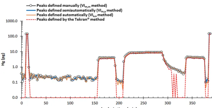
Figure 2.Test dataset collected with a Tekran®2537A instrument, represented as Hg loadings derived from my VI-based manual, semiau-tomated, and automated Hg thermal desorption peak height determination methods (the VIm,m, VIm,a, and VIa,amethods, respectively) and by the Tekran®method. Peaks not detected by the Tekran®method are assigned a value of 0.01 pg. The two pairs of data points at>100 pg correspond with calibration gas analysis cycles (SPAN samples). I use the first pair of SPAN samples to initialize the VI (as described in Sect. 2.2). I use response factors calculated from the second pair of SPAN samples (and the preceding pair of blanks) to calculate Hg load-ings for all other samples in the dataset. The mean value of the baseline standard deviation,σbl(defined in Sect. 2.1), is∼0.03 mV (equal to
∼0.03 pg). The corresponding estimated lower-limitf value (mean±2σ; Sect. 2.3) is 1.86(1)×10−4.
are assigned (paired by Au trap identity) to all samples in the data file to be processed.
2.3 Automatic determination of the Hg thermal
desorption peak end time
It is necessary to define each Hg thermal desorption peak’s end time,tend, within the interval during which the Tekran®
analyzer’s Hg atomic fluorescence signal is recorded (38.9 s in Figs. 1a and S4a). Therefore, for each sample the VI de-finestendas the time at whichS(t )decays to a value equal to,
or less than, a fraction,f, of the amplitude,ASPAN(derived
as in Sect. 2.2), determined from a calibration gas analysis cycle on the same Au trap:
S (tend)≤(f×ASPAN)+Soffset. (2)
Substituting the right-hand side of Eq. (2) forS(t )in Eq. (1) and solving fort (=tend)yields an analytical expression for
the upper-bound value oftend:
tend=ln
f ×ASPAN Ai
×b−1∼=ln
f×ASPAN Hi
×b−1.
(3) Here,Ai andHi are the TD peak amplitude and the initial
peak height (from step 6 in Sect. 2.1), respectively, of the sample for which the baseline-slope-corrected peak height is to be quantified. The partial equality in Eq. (3) reflects the facts thatASPAN/Ai∼=HSPAN/HiandASPAN∼=HSPAN. The
Au-trap-dependent value of the decay constant,b, is derived as in Sect. 2.2.
The value off is chosen such thattendis≥0 at the
small-est expected value ofHi, which the VI approximates asσbl
(Sect. 2.1). The upper-bound value off is estimated sepa-rately for each Au trap by solving Eq. (3) forf, withtend=0
andHi=σbl: f =
σbl ASPAN
. (4)
The Au-trap-dependentf values are then averaged prior to application in Eq. (3). I estimate the uncertainty inf to be twice the standard deviation in the mean for the two Au traps. Uncertainty in the value of Hi is estimated to be equal to
twice the baseline standard deviation calculated in step 9 of Sect. 2.1. Uncertainty in the automatically derived value of tend,δtend, is estimated by propagating uncertainties inb,f,
andHithrough Eq. (3) (see below).
It is necessary to further constraintend such that for large
TD peaks (e.g., those recorded for SPAN samples) the au-tomatically determined value oftend is at least 10 ds before
the upper-bound time, tn, of the interval during which the
instrument’s Hg AF signal is recorded. The VI therefore de-finestend as the smaller of the results of Eq. (3) andtn−10,
wherenrepresents the number of AF signal values recorded (n=389 in Figs. 1a and S4a). A minimum value of 10 ds is also prescribed fortendsuch that for very small TD peaks the
automatically determined peak end does not occur at or be-fore the peak max time (e.g., whenf ≥Hi/ASPANin Eq. 3).
Figure 3. (a)Comparison of Hg loadings derived from measurements made with a Tekran®2537A instrument using the Tekran®method and my VI-based Hg thermal desorption peak height determination method (dataset shown in Fig. 2, excluding SPANs), with the peaks defined manually (the VIm,mmethod). The equation of the linear regression isy=1.00(1)x−0.45(8)pg (r2=0.997,n=74). The fit excludes data derived from peaks not detected by the Tekran®method (represented by the open symbols).(b)Absolute and relative biases in the Tekran®-derived Hg loadings, based on the fit in panel(a). The grey bands represent propagated uncertainties (95 % confidence intervals) in the fit parameters.(c)Distribution of residuals from panel(a), including only data derived from detected peaks. (Analogous results for the 2537B instrument are presented in Fig. S5.)
Table 1.Bias in Hg loadings derived by applying automated and semiautomated Hg atomic fluorescence signal processing methods to measurements made with a Tekran®2537A instrument.
Method Hg (pg, ng m−3)1,2
7.5, 1.5 3.75, 0.75 2.5, 0.5 1.25, 0.25 0.5, 0.1 0.25, 0.05 0.125, 0.025
Bias (%)
Tekran®3 −6±2 −12±2 −18±3 −36±6 −1006 −1006 −1006 VI4a,a 0.1±0.2 0.1±0.2 0.1±0.3 0.2±0.5 0.3±1.2 0.6±2.3 1±5 VI5m,a 0.15±0.08 0.2±0.1 0.3±0.1 0.5±0.3 1.0±0.6 2±1 4±2
1Bias values for the Tekran®and VI
a,amethods are calculated from the equations of the linear regressions in Figs. 3a and 5a, respectively. Bias values for the VIm,amethod are similarly calculated from the linear regression equation given in Table S4 (“standard” configuration). All bias values are expressed relative to Hg loadings derived by processing the data using manual peak definition (the VIm,mmethod);2Hg loadings are also expressed in terms of concentrations under the typical Tekran®operating parameters;3Tekran®operating and peak integration parameters are defined in Table S1;4my VI-based peak height determination method, with peak start and end times determined automatically (VIa,a);5my VI-based peak height determination method, with peak start times determined manually and peak end times determined automatically (VIm,a);6for Hg<the estimated 0.8 pg Tekran®limit of detection, the true bias is−100 %. For clarity, the true bias is substituted for the calculated values.
2.4 Evaluation
I evaluate the performances of the VIm,aand VIa,amethods
by applying both methods to laboratory data collected with two Tekran® analyzers (one model 2537A and one model 2537B). One dataset is processed for each analyzer. The test dataset collected with the 2537A instrument is shown in Fig. 2. (The test dataset for the 2537B instrument is shown in Fig. S3.)
I consider the manual definition of the Hg thermal des-orption peaks (the VIm,m method) to be the benchmark for
signal processing accuracy, and I assess the accuracies of the VIm,aand VIa,amethods by comparing Hg sample loadings
derived from both methods with loadings derived from the VIm,mmethod. A similar comparison is used to evaluate the
accuracy of the Tekran® method. The performances of all methods are further evaluated and compared based on the Hg limits of detection (LODs) they achieve.
3 Results and discussion: performance evaluations
3.1 The Tekran®Hg thermal desorption peak
integration method
For Hg loadings derived from the Tekran® method, HgTekran, I define absolute bias as HgTekran−Hgbenchmark,
where Hgbenchmark represents loadings derived from the
VIm,m method. I define relative bias as 100×(HgTekran−
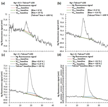
Figure 4.Comparison of Hg fluorescence baselines calculated by applying manual (VIm,mmethod), automated (Tekran®and VIa,amethods), and semiautomated (VIm,amethod) Hg thermal desorption peak definition methods to samples with Hg loadings of approximately(a)0.5,
(b)1,(c)2, and(d)4 times the limit of detection of the Tekran®method (∼0.8 pg). Measurements were made with a 2537A instrument. Biases in the Hg loadings derived from the Tekran®method and the VI-based methods are indicated. Biases are expressed relative to the loadings derived from the VIm,mmethod and are negative when the VIm,m-based loadings are higher. The Tekran®baselines are missing from panels(a)and(b)because the peaks are not detected by the Tekran®method.
Fig. S5), Hg loadings derived using the Tekran®method tend to be biased low, with the relative bias becoming more neg-ative with decreasing loading. I present in Table 1 relneg-ative bias values from Fig. 3b at several discrete Hg sample load-ings (analogous results for the 2537B dataset are presented in Table S2). The corresponding Hg concentrations (ng m−3) under typical operating conditions for the Tekran®analyzer (5 L sample volumes) are also shown. My results are consis-tent with those of Swartzendruber et al. (2009) and Slemr et al. (2016) but also demonstrate that the Tekran®method can produce significant low biases (≥5 %; see Tables 1 and S2) at tropospheric background GEM and THg concentrations (∼1 to 2 ng m−3; sample loadings of 5–10 pg under typical Tekran®operating conditions).
To further characterize the performance of the Tekran® method, Fig. 4 compares Hg atomic fluorescence baselines
calculated by the Tekran®method and by my VI-based peak height determination methods for samples with Hg loadings of approximately 0.5, 1, 2, and 4 times the estimated∼0.8 pg LOD achieved with the Tekran® method (see below). (See Sect. S6 for details on how I reproduced the baselines calcu-lated by the Tekran® method.) Figure 4 illustrates the ten-dency of the Tekran® method to truncate the Hg thermal desorption peaks. The peaks tend to become more severely truncated as they become smaller, and as a result, the rela-tive biases in the corresponding Hg loadings tend to become more negative as the loadings decrease, as shown in Figs. 3b and S5b (see also Fig. 2 in Slemr et al., 2016).
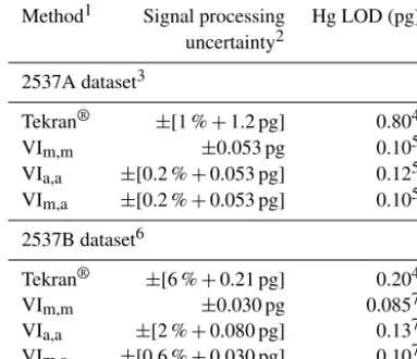
load-method and my VI-based peak height determination load-methods as ap-plied to measurements made with Tekran®2537A and 2537B in-struments.
Method1 Signal processing Hg LOD (pg) uncertainty2
2537A dataset3
Tekran® ±[1 %+1.2 pg] 0.804 VIm,m ±0.053 pg 0.105 VIa,a ±[0.2 %+0.053 pg] 0.125 VIm,a ±[0.2 %+0.053 pg] 0.105
2537B dataset6
Tekran® ±[6 %+0.21 pg] 0.204 VIm,m ±0.030 pg 0.0857 VIa,a ±[2 %+0.080 pg] 0.137 VIm,a ±[0.6 %+0.030 pg] 0.107
1The Tekran®method is the Tekran®analyzer’s internal automated Hg thermal desorption peak integration method, parameterized as indicated in Table S1. The VIm,m, VIa,a, and VIm,aHg TD peak height determination methods were developed in this work and are described in Sect. 2. The operating parameters of the Tekran® analyzers are presented in Table S1;2estimated as described in Sect. 3.4;3the 2537A dataset is shown in Fig. 2;4estimated as the highest Hg loading derived from the VIm,mmethod for samples for which the Tekran®method failed to detect the Hg TD peak; 5estimated as twice the standard deviation of blank loadings
(n=62).6The 2537B dataset is shown in Fig. S3.7Estimated as twice the standard deviation of blank loadings (n=37).
ings >10 times higher (see Figs. 2 and S3, respectively). Calibrating the measurements in Fig. S5a using the exter-nal SPANs (Fig. S3; loadings >5 times higher) yields the linear regression equation (as in Fig. S5a) y=0.96(1)x− 0.09(5)pg. The slope of the latter equation is closer to unity (though not significantly) than that of the equation derived from Fig. S5a.
Table 2 presents Hg LODs for the Hg fluorescence sig-nal processing methods and datasets I tested. The nomisig-nal Hg limit of detection of the Tekran®analyzer is 0.5 pg (see Sect. S7 for further details). However, some Hg thermal des-orption peaks in the 2537A dataset are undetected by the Tekran®method for Hg loadings≤0.8 pg (Figs. 2 and 3a). My results suggest that the actual Hg LOD achieved with the Tekran® method is ∼60 % higher than the nominal value. By comparison, the LOD achieved with the VIm,mmethod
(estimated as twice the standard deviation of blank samples, n=62) is 0.10 pg.
For the 2537B dataset, all Hg thermal desorption peaks are detected by the Tekran® method for Hg loadings >0.2 pg (Figs. S3 and S5), suggesting the LOD is∼60 % lower than the nominal value. The lower Hg LOD achieved with the Tekran® method when applied to the 2537B dataset is at-tributable to the hardware modifications that were made to the 2537B instrument to increase its signal-to-noise ratio
3.2 The automated VI-based Hg thermal desorption
peak height determination method
By comparison with the Tekran®method, the VIa,amethod
usually identifies the Hg thermal desorption peak baseline with good accuracy, even at Hg loadings near to or below the LOD achieved with the Tekran®method (Fig. 4). As a result, most Hg loadings derived from the VIa,a method are quite
accurate (Figs. 2 and 5; Table 1). For samples with Hg load-ings below the estimated 0.8 pg LOD of the Tekran®method, the mean absolute and relative unsigned biases in the load-ings derived from the VIa,amethod are 0.028±0.005 pg and
15±3 %, respectively (n=78). The biases are very small and much smaller in magnitude than those for the Tekran®
method (estimated at−0.80 pg and−100 %). Based on the equations of the linear regressions shown in Figs. 3a and 5a (Hg loadings≤10 pg), the VIa,amethod achieves≥94 %
re-duction in absolute unsigned bias in calculated Hg loadings when compared with the Tekran®method.
The Hg LOD achieved with the VIa,a method is 0.12 pg
(estimated as twice the standard deviation of blank values; n=62). That value is 20 % higher than the LOD achieved with the VIm,m method but 85 % lower than the LOD
achieved with the Tekran®method (Table 2). Similarly, the width of the residual distribution in Fig. 5c is 78 % narrower than that in Fig. 3c, which reflects the improved analytical precision achieved with the VIa,amethod in comparison with
the Tekran®method.
Evaluation of the VIa,amethod as in Fig. 5 for the 2537B
dataset (Fig. S6, Table S2) yields the linear regression equa-tion y=1.015(2)x−0.017(8)pg (r2=0.9998, n=132). For samples with Hg loadings below 0.8 pg, the observed mean absolute and relative unsigned biases in the loadings derived from the VIa,a method are 0.031±0.007 pg and
33±9 %, respectively (n=41). The VIa,a method yields a
larger relative bias when applied to the 2537B dataset than when applied to the 2537A dataset. However, absolute un-signed biases are equivalent (at the 95 % confidence inter-val) for the two datasets. Based on the equations of the lin-ear regressions shown in Figs. S5a and S6a, the VIa,amethod
achieves≥82 % reduction in absolute unsigned bias in calcu-lated Hg loadings when compared with the Tekran®method. The Hg LOD is 0.14 pg (Table 2), which is 59 % higher than the value achieved with the VIm,mmethod but 31 % lower
than the value achieved with the Tekran®method. The VIa,a
Figure 5. (a)Comparison of Hg loadings derived from measurements made with a Tekran®2537A instrument using my VI-based automated and manual peak height determination methods (the VIa,aand VIm,mmethods, respectively; dataset shown in Fig. 2, excluding SPANs). The equation of the linear regression isy=1.001(1)x+0.000(6)pg (r2=0.99992,n=152).(b)Absolute and relative biases in the VI-based Hg loadings, based on the fit in panel(a); grey bands represent propagated uncertainties (95 % confidence intervals) in the parameters of the fit in panel(a).(c)Distribution of residuals from panel(a).
3.3 The semiautomated VI-based peak height
determination method
The VIa,amethod poorly identifies the start of the Hg thermal
desorption peak for some blank samples with the lowest Hg loadings. As a result, the Hg TD peak height and the calcu-lated Hg loading tend to be underestimated for those samples (Figs. 2 and S3).
I developed the VIm,a method as a compromise between
the Hg TD peak definition accuracy achieved with the VIm,m
method and the data processing speed achieved with the VIa,a
method. (Peak height determination for a single sample re-quires from<1 s with the VIa,a method to several seconds
for the VIm,mmethod; the data processing time for the VIm,a
method is approximately half that for the VIm,m method.)
Comparison of the VIm,a and VIa,a results in Fig. 2 (and
Fig. S3) shows that defining tstart manually instead of
au-tomatically yields more accurate measurements for samples with the lowest Hg loadings.
Evaluation of the VIm,amethod as in Fig. 5 yields the
lin-ear regression equation y=1.001(1)x+0.004(3)pg (r2= 0.99998,n=152). Comparison between the latter equation and that of the regression in Fig. 5a suggests that biases in Hg loadings derived from the VIa,a and VIm,a methods
are not significantly different over the range of loadings in the 2537A dataset (see also Table 1). However, biases in Hg loadings derived from the VIm,a method are lower at
low loadings than those determined for the VIa,a method
(Sect. 3.2): for samples with Hg loadings below 0.8 pg, the mean absolute and relative unsigned biases in the loadings derived from the VIm,a method are 0.012±0.003 pg and
6±1 %, respectively (n=78). The estimated 0.10 pg Hg LOD achieved with the VIm,a method is equivalent to that
achieved with the VIm,mmethod (Table 2).
The VIm,a method performs consistently better for the
2537B dataset than does the VIa,a method. The equation
of the linear regression (as in Fig. 5a) isy=1.005(1)x+ 0.009(5)pg (r2=0.99994,n=132). For samples with Hg loadings below 0.8 pg, the observed mean absolute and rel-ative unsigned biases in the loadings derived from the VIm,a
method are 0.010±0.003 pg and 6±2 %, respectively (n= 41). The estimated LOD achieved with the VIm,amethod is
0.10 pg and falls between the LODs achieved with the VIm,m
and VIa,amethods (Table 2).
3.4 Sensitivity analyses and uncertainties
To test the sensitivity to initialization parameters of Hg load-ings derived from the VIa,a and VIm,a methods, I
recalcu-lated those loadings after making a series of modifications to the method initialization parameters. After each modifica-tion I recalculated the parameters of the Hg regression (e.g., Fig. 5a). The modifications tested for the 2537A dataset (de-scribed further in Tables S3 and S4) include shifts intendby
±δtend (as defined in Sect. 2.3), shifts in tstart to the
val-ues determined (as described in Sect. 2.2) for the second pair of SPAN samples in Fig. 2 (applicable only to the VIa,a
method), and initialization of the VI using the second pair of SPAN samples. (Details on the sensitivity tests applied to the 2537B dataset are described in Tables S5 and S6.)
The above modifications result in insignificant changes (at the 95 % confidence interval) to the bias parameters derived (as in Fig. 5a) for the VIa,amethod and the 2537 dataset
(Ta-ble S3). Two sensitivity tests applied to the VIa,amethod and
the 2537B dataset result in significant changes (at the 95 % confidence interval) to the calculated bias parameters (Ta-ble S5). Results obtained with the VIa,a method therefore
(Table 2). It is possible that a large shift in tstartfor SPAN
samples over the course of an analysis would increase the sensitivity of the VIa,a method to initialization parameters.
Results obtained with the VIm,a method are insensitive (at
the 95 % confidence interval) to initialization parameters (Ta-bles S4 and S6).
I estimate signal processing uncertainties in the Hg ther-mal desorption peak heights derived from the VIm,mmethod
to be equal to twice the mean baseline standard deviation (σbl, Sect. 2.1), corresponding with a Hg loading of 0.053 pg
for the dataset in Fig. 2 (0.030 pg for the dataset in Fig. S3). I estimate signal processing uncertainties in the Hg loadings derived from the Tekran®, VIa,a, and VIm,amethods as the
sum of the biases in those methods (derived as in Fig. 3) and the resulting increase (relative to the VIm,mmethod) in the
Hg limit of detection (Table 2). For the VIa,aand VIm,a
meth-ods, I estimate a conservative threshold uncertainty value of ±2σbl.
Signal processing uncertainty attributable to my VIa,a
method, as applied to the 2537A dataset, is estimated to be within ±[0.2 %+0.053 pg]. (The first term in the lat-ter expression represents the slope of the regression in Fig. 5a; the second term represents 2σbl, which in this case
is larger than the sum of the 0.000±0.006 pg intercept of the fit in Fig. 5a and the 0.02 pg difference in Hg LODs achieved with the VIa,aand VIm,mmethods). Estimated
sig-nal processing uncertainty attributable to the VIm,a method
is also within ±[0.2 %+0.053 pg]. By comparison, signal processing uncertainty attributable to the Tekran® method is within±[1 %+1.2 pg]. The above uncertainty results, to-gether with estimated Hg LODs and analogous results for the 2537B dataset, are summarized in Table 2. For both test datasets, signal processing uncertainties estimated for my VI-based methods are significantly lower than those for the Tekran®method. Signal processing uncertainty ranks as fol-lows for the VI-based methods: VIm,m<VIm,a≤VIa,a.
4 Conclusions and implications
I describe three improved methods for processing the raw Hg atomic fluorescence signal from Tekran® 2537A and 2537B Hg vapor analyzers. The methods incorporate man-ual, semiautomated, or fully automated Hg thermal desorp-tion peak identificadesorp-tion processes. I implement my methods through a virtual instrument in National Instruments™ Lab-VIEW and evaluate them, together with the Tekran®internal Hg TD peak integration method, using test datasets from two Tekran®instruments (one 2537A and one 2537B).
Consistent with previous work (Swartzendruber et al., 2009; Slemr et al., 2016), my results demonstrate that Hg loadings derived from the Tekran®method tend to be biased low, with the relative bias becoming more negative with
de-on sampling cde-onditide-ons (e.g., sample cde-oncentratide-on and vol-ume). Therefore, I recommend that signal processing bias be examined, and associated uncertainties be quantified, in all future applications of the Tekran®instruments, regardless of sampling arrangement.
With respect to atmospheric GEM and THg measure-ments, my results demonstrate that the Tekran®method can produce significant low biases (≥5 %) at background con-centrations (∼1 to 2 ng m−3)under typical operating condi-tions (Hg loadings of 5–10 pg). My results therefore indicate that post-processing the raw Tekran®data can yield signifi-cant improvements in the accuracy of the derived Hg concen-trations under much broader environmental conditions than previously recognized. Such conditions should not be as-sumed to be limited to those where GEM concentrations can be significantly depleted, as can occur in the free troposphere and lower stratosphere (e.g., Talbot et al., 2007; Lyman and Jaffe, 2012; Timonen et al., 2013; Gratz et al., 2015), as well as at the surface in polar and midlatitude regions under spe-cial photochemical conditions (e.g., Schroeder et al., 1998; Obrist et al., 2011).
Most measurements of atmospheric GOM and PBM made with the Tekran® 1130/1135 Hg speciation system (Lan-dis et al., 2002) may be significantly biased low. For in-stance, typical median GOM and PBM concentrations mea-sured at 21 Atmospheric Mercury Network (AMNet) sites in the United States and Canada during the years 2009–2011 were in the ranges 1.2–2.5 and 2.5–5.0 pg m−3, respectively (Gay et al., 2013). The corresponding Hg loadings are 1.4– 3.0 and 3.0–6.0 pg. The median signal processing bias, es-timated as 100×(HgTekran−Hgbenchmark)/HgTekran, would be within−39 and−19 %, respectively, based on the fit in Fig. 3a, and within−17 and−12 %, respectively, based on the fit in Fig. S5a. Similarly, median concentrations of GOM and/or PBM measured at 10 sites in Canada during the years 2002–2011 were typically <5 pg m−3 (Cole et al., 2014), corresponding with sample loadings of 3–9 pg. The corre-sponding median signal processing bias would be within−19 and−8 %, respectively, based on the fit in Fig. 3a, and within −12 and−8 %, respectively, based on the fit in Fig. S5a.
My results suggest that the performance of the Tekran® method may be improved with hardware modifications that increase the instrument’s signal-to-noise ratio. The Tekran® method performs better at low Hg loading when applied to the 2537B dataset than when applied to the 2537A dataset. The primary difference between the 2537A and 2537B in-struments I tested is that the 2537B instrument was modified to improve its signal-to-noise ratio by replacing the sample cuvette and detector bandpass filter with a mirrored cuvette and an improved filter, respectively (Ambrose et al., 2013). It is possible that the performance of the Tekran®method can also be improved through modification of the method’s inte-gration parameters, though I tested only the default parame-ters (Table S1). Additionally, it is possible that measurement bias introduced by the Tekran®method can be made smaller by calibrating at loadings more similar to the loadings in the samples of interest. My results demonstrate a minor reduc-tion in bias when measurements made with the 2537B in-strument are calibrated at loadings that are>5 times higher rather than at loadings>10 times higher. Measurement bias and precision can in principle both be improved by employ-ing longer sample preconcentration times and/or higher sam-ple flow rates to achieve higher samsam-ple loadings.
Estimated signal processing uncertainties in Hg loadings derived from my methods range from within ±0.053 pg when the Hg thermal desorption peaks are defined man-ually to within ±[0.2 %+0.053 pg] (2537A dataset) and ±[2 %+0.080 pg] (2537B dataset) when Hg TD peak defini-tion is fully automated. Biases in Hg loadings derived from my methods are lower by>80 % than biases derived from the Tekran® method. Limits of detection for Hg decrease by 31 to 88 % when my methods are used in place of the Tekran®method.
Data availability. The primary data used in this work are archived in the Open Science Framework repository (https://doi.org/10.17605/OSF.IO/KGFYP, Ambrose, 2017).
The Supplement related to this article is available online at https://doi.org/10.5194/amt-10-5063-2017-supplement.
Competing interests. The author declares that he has no conflict of interest.
Acknowledgements. Financial support for the Hg science com-ponent of NOMADSS was provided by the US National Science Foundation, award no. 1217010. I would like to thank the Jaffe Research Group for the helpful discussions during manuscript preparation as well as Franz Slemr for his constructive review.
Edited by: Robyn Schofield
Reviewed by: Franz Slemr and two anonymous referees
References
Ambrose, J.: Data Archive for: Improved methods for sig-nal processing in measurements of mercury by Tekran® 2537A and 2537B instruments, Open Science Framework, https://doi.org/10.17605/OSF.IO/KGFYP, 2017.
Ambrose, J. L., Reidmiller, D. R., and Jaffe, D. A.: Causes of high O3 in the lower free troposphere over the Pacific Northwest as observed at the Mt. Bachelor Observatory, Atmos. Environ., 45, 5302–5315, https://doi.org/10.1016/j.atmosenv.2011.06.056, 2011.
Ambrose, J. L., Lyman, S. N., Huang, J., Gustin, M. S., and Jaffe, D. A.: Fast time resolution oxidized mercury measure-ments during the Reno Atmospheric Mercury Intercomparison Experiment (RAMIX), Environ. Sci. Technol., 47, 7285–7294, https://doi.org/10.1021/es303916v, 2013.
Ambrose, J. L., Gratz, L. E., Jaffe, D. A., Campos, T., Flocke, F. M., Knapp, D. J., Stechman, D. M., Stell, M., Weinheimer, A. J., Cantrell, C. A., and Mauldin III, R. L.: Mercury emission ratios from coal-fired power plants in the southeastern United States during NOMADSS, Environ. Sci. Technol., 49, 10389–10397, https://doi.org/10.1021/acs.est.5b01755, 2015.
Cole, A. S., Steffen, A., Eckley, C. S., Narayan, J., Pilote, M., Tor-don, R., GrayTor-don, J. A., St. Louis, V. L., Xu, X., and Bran-fireun, B. A.: A Survey of Mercury in Air and Precipitation across Canada: Patterns and Trends, Atmosphere, 5, 635–668, https://doi.org/10.3390/atmos5030635, 2014.
Gay, D. A., Schmeltz, D., Prestbo, E., Olson, M., Sharac, T., and Tordon, R.: The Atmospheric Mercury Network: measure-ment and initial examination of an ongoing atmospheric mercury record across North America, Atmos. Chem. Phys., 13, 11339– 11349, https://doi.org/10.5194/acp-13-11339-2013, 2013. Gratz, L. E., Ambrose, J. L., Jaffe, D. A., Shah, V., Jaeglé, L.,
Stutz, J., Festa, J., Spolaor, M., Tsai, C., Selin, N. E., Song, S., Zhou, X., Weinheimer, A. J., Knapp, D. J., Montzka, D. D., Flocke, F. M., Campos, T. L., Apel, E., Hornbrook, R., Blake, N. J., Hall, S., Tyndall, G. S., Reeves, M., Stechman, D., and Stell, M.: Oxidation of mercury by bromine in the subtropical Pacific free troposphere, Geophys. Res. Lett., 42, 10494–10502, https://doi.org/10.1002/2015GL066645, 2015.
Gustin, M. S. and Jaffe, D.: Reducing the uncertainty in measure-ment and understanding of mercury in the atmosphere, Environ. Sci. Technol., 44, 2222–2227, 2010.
Jaffe, D. J., Prestbo, E., Swartzendruber, P., Weiss-Penzias, P., Kato, S., Takami, A., Hatakeyama, S., and Kajii, Y.: Export of atmo-spheric mercury from Asia, Atmos. Environ., 39, 3029–3038, 2005.
Feddersen, D., Horvat, M., Dastoor, A., Hynes, A. J., Mao, H., Sonke, J. E., Slemr, F., Fisher, J. A., Ebinghaus, E., Zhang, Y., and Edwards, G.: Progress on understanding atmospheric mer-cury hampered by uncertain measurements, Environ. Sci. Tech-nol., 48, 7204–7206, https://doi.org/10.1021/es5026432, 2014. Landis, M. S., Stevens, R. K., Schaedlich, F., and Prestbo, E.
M.: Development and characterization of an annular denuder methodology for the measurement of divalent inorganic reac-tive gaseous mercury in ambient air, Environ. Sci. Technol., 36, 3000–3009, 2002.
Lyman, S. N. and Jaffe, D. A.: Formation and fate of oxidized mer-cury in the upper troposphere and lower stratosphere, Nature Geosci., 5, 114–117, https://doi.org/10.1038/ngeo1353, 2012. Obrist, D., Tas, E., Peleg, M., Matveev, V., Faïn, X., Asaf,
D., and Luria, M.: Bromine-induced oxidation of mercury in the mid-latitude atmosphere, Nature Geosci., 4, 22–26, https://doi.org/10.1038/NGEO1018, 2011.
Pandy, S. K., Kim, K.-H., and Brown, R. J. C.: Measurement tech-niques for mercury species in ambient air, TrAC-Trend, Anal. Chem., 30, 899–917, https://doi.org/10.1016/j.trac.2011.01.017, 2011.
Pirrone, N., Aas, W., Cinnirella, S., Ebinghaus, R., Hedge-cock, I. M., Pacyna, J., Sprovieri, F., and Sunder-land, E. M.: Toward the next generation of air qual-ity monitoring: Mercury, Atmos. Environ., 80, 599–611, https://doi.org/10.1016/j.atmosenv.2013.06.053, 2013.
Schroeder, W. H., Keeler, G., Kock, H., Roussel, P., Schneeberger, D., and Schaedlich, F.: International field intercomparison of at-mospheric mercury measurement methods, Water Air Soil Poll., 80, 611–620, 1995.
Schroeder, W. H., Anlauf, K. G., Barrie, L. A., Lu, J. Y., Steffen, A., Schneeberger, D. R., and Berg, T.: Arctic springtime depletion of mercury, Nature, 394, 331–332, 1998.
ber, S., Hermann, M., Becker, J., Zahn, A., and Martins-son, B.: Atmospheric mercury measurements onboard the CARIBIC passenger aircraft, Atmos. Meas. Tech., 9, 2291–2302, https://doi.org/10.5194/amt-9-2291-2016, 2016.
Stratton, W. J. and Lindberg, S. E.: Use of a refluxing mist chamber for measurement of gas-phase mercury(II) species in the atmo-sphere, Water Air Soil Poll., 80, 1269–1278, 1995.
Swartzendruber, P., Jaffe, D. A., and Finley, B.: Improved fluores-cence peak integration in the Tekran 2537 for applications with suboptimal sample loadings, Atmos. Environ, 43, 3648–3651, 2009.
Talbot, R., Mao, H., Scheuer, E., Dibb, J., and Avery, M.: Total depletion of Hg◦ in the upper troposphere-lower stratosphere, Geophys. Res. Lett, 34, L23804, https://doi.org/10.1029/2007GL031366, 2007.
Tekran Corporation: Model 2537A Ambient Mercury Vapour Ana-lyzer User Manual, Rev. 3.01, Tekran Instruments Corporation, Toronto, Canada, 2006.
Tekran Corporation: Model 2537B Ambient Mercury Vapor Ana-lyzer User Manual, Rev. 3.10, Tekran Instruments Corporation, Toronto, Canada, 2007.
Timonen, H., Ambrose, J. L., and Jaffe, D. A.: Oxidation of el-emental Hg in anthropogenic and marine airmasses, Atmos. Chem. Phys., 13, 2827–2836, https://doi.org/10.5194/acp-13-2827-2013, 2013.