Dynamics of simple earthquake model with time delay and variation of friction strength

(1)

www.nonlin-processes-geophys.net/20/857/2013/ doi:10.5194/npg-20-857-2013

Nonlinear Processes

in Geophysics

Dynamics of simple earthquake model with time delay and variation

of friction strength

S. Kostić1, N. Vasović1, I. Franović2, and K. Todorović3

1_{University of Belgrade Faculty of Mining and Geology, Ðušina 7, Belgrade, Serbia} 2_{University of Belgrade Faculty of Physics, Studentski trg 12, Belgrade, Serbia} 3_{University of Belgrade Faculty of Pharmacy, Vojvode Stepe 450, Belgrade, Serbia}

Correspondence to: S. Kosti´c ([email protected])

Received: 23 December 2012 – Revised: 10 September 2013 – Accepted: 15 September 2013 – Published: 29 October 2013

Abstract. We examine the dynamical behaviour of the phe-nomenological Burridge–Knopoff-like model with one and two blocks, where the friction term is supplemented by the time delayτ and the variable friction strength c. Time de-lay is assumed to reflect the initial quiescent period of the fault healing, considered to be a function of history of slid-ing. Friction strength parameter is proposed to mimic the im-pact of fault gouge thickness on the rock friction. For the single-block model, interplay of the introduced parametersc andτ is found to give rise to oscillation death, which cor-responds to aseismic creeping along the fault. In the case of two blocks, the action ofc1,c2,τ1andτ2may result in

sev-eral effects. If both blocks exhibit oscillatory motion with-out the included time delay and frictional strength parame-ter, the model undergoes transition to quasiperiodic motion if onlyc1andc2are introduced. The same type of behaviour

is observed whenτ1 andτ2 are varied under the condition c1=c2. However, ifc1, andτ1are fixed such that the given

block would lie at the equilibrium whilec2andτ2 are

var-ied, the (c2, τ2)domains supporting quasiperiodic motion are

interspersed with multiple domains admitting the stationary solution. On the other hand, if (c1, τ1)warrant oscillatory

be-haviour of one block, under variation ofc2andτ2 the

sys-tem’s dynamics is predominantly quasiperiodic, with only small pockets of (c2, τ2)parameter space admitting the

peri-odic motion or equilibrium state. For this setup, one may also find a transient chaos-like behaviour, a point corroborated by the positive value of the maximal Lyapunov exponent for the corresponding time series.

1 Introduction

Earthquakes represent complex deformation feature of the Earth’s brittle crust. Their complexity reveals itself primar-ily in the power-law scaling describing the distribution of magnitudes (Turcotte et al., 2000), fractal spatial distribution of epicentres and fractal-like structure of faults (Okubo and Aki, 1987; Marsan et al., 2000). Nonetheless, earthquakes also involve complex patterns of temporal behaviour, which may be manifested by the chaotic dynamics in the recorded seismic time series (Beltrami and Mareshal, 1993). A plau-sible explanation for this complexity lies in that it is gener-ated by nonlinear dynamics on a smooth fault, a point first raised by Horowitz and Ruina (1989). This line of research was followed by Carlson and Langer (1989) in the work on dynamics of Burridge–Knopoff arrays of spring-connected blocks with classical velocity-weakening friction laws. Also, Bak and Tang (1989) investigated a simple cellular-automata model of the failure at a critical stress. However, though all these approaches consider earthquakes from the phenomeno-logical standpoint, there is still no general consensus on what constitutes the right model for describing the motions of earthquake faults. Therefore, it is useful to study a variety of models and, in doing so, learn how their various ingredi-ents determine the behaviour that they exhibit (Langer et al., 1996).

(2)

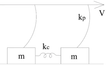
Fig. 1. Burridge–Knopoff model with two blocks. Parameterm rep-resents the mass of the block,kcandkp are the spring constants, andV denotes the velocity of the driving plate.

direct associations between the parameters involved and the observations of the real seismic phenomena. The first con-tinuum model of the latter type was proposed by Burridge and Knopoff (1967). This spring-block model, coupled with the appropriate friction law, is capable of generating power-law distribution of energy release, described by Gutenberg– Richter and Omori–Utsu laws (Burridge and Knopoff, 1967). The model consists of several blocks interconnected with springs of some elastic constantk, having the blocks also attached by a leaf spring to a driving plate, that causes the whole system to move along the rough surface in a stick-slip fashion (Fig. 1).

Apart from accounting for the statistical power-law distri-bution of released energy (Burridge and Knopoff, 1967), this model has been shown to exhibit rich dynamical behaviour (Carlson and Langer, 1989; De Sousa Vieira, 1995, 1999; Er-ickson et al., 2008). Carlson and Langer (1989) have demon-strated that chaotic dynamics may arise as a direct conse-quence of the friction law, which effectively causes small irregularities in the system to be amplified during the slip-ping motions. Their model produces three qualitatively dis-tinct kinds of slipping events: microscopic events, large but localised events and delocalised great events. On the other hand, De Sousa Vieira (1999) analysed rich dynamical be-haviour in a two block system, having identified the period-doubling route to chaos. Erickson et al. (2008) reported that in a spring-block model with only one block coupled with the Dieterich–Ruina friction law chaotic behaviour also emerges via the Feigenbaum scenario.

All the research mentioned so far relies on the notion that the behaviour of the considered model is essentially con-trolled by the chosen friction law. Initially, Burridge and Knopoff (1967) in their original model used a simple fric-tion law, where the fricfric-tion force is dependent on the veloc-ity of the block relative to the frictional surface. The main feature of this law is that the friction has to decrease more or less suddenly as the velocity deviates from zero, whereas for very small velocities, friction may attain any value less than the limiting friction. Afterwards, slip rate and state vari-able constitutive laws for rock friction were developed and

introduced by Dieterich (1979), Ruina (1983) and Rice (Rice, 1983; Rice and Ruina, 1983). These early studies were de-signed to study frictional instability as a possible mechanism for the repetitive stick-slip failure and the seismic cycle. In this paper, we assume that the friction force at the contact of a block and a rough surface depends only on the velocity of the block. However, recalling that many experimental ob-servations indicate that the rock friction also depends on the state of the contact surface (Marone, 1998), we introduce this memory effect by including the time delay parameterτin the friction term. The role of this parameter is twofold. Firstly, it replaces the state variable θ incorporated in the Dieterich– Ruina friction law, which is usually interpreted as a function of history of sliding (Pomeau and Le Berre, 2011). Secondly, this time delay effect is directly observed both in laboratory experiments and along the real fault. According to the re-sults of laboratory tests, upon the cessation of motion, static friction shows an initial period of retarded healing for a few hundred days, after which an increase in healing is observed (Marone, 1998). Moreover, it is determined that the length of this initial period of delayed healing varies with stiffness, which justifies our variation of the introduced time delay pa-rameterτ. These laboratory results are further corroborated by seismic data, which indicate that the healing rate is re-duced during the period immediately following earthquakes of similar size (less than 10–100 days after the last earth-quake), with the small variations in the stress drop.

One should point out that this retarded initial period of fault healing is reminiscent of the refractory stage of the relaxation oscillators. Modelling the behaviour of spatially extended media comprised of relaxation oscillators often in-volves the delay-differential equations. Such an approach is widely accepted, particularly in the fields of mathematical biology (Golpasamy and Leung, 1996; Buri´c and Todorovi´c, 2002) and life sciences (Smith, 2011).

(3)

thickness of fault gouge on the dynamical stability of motion along the fault. Also, by assuming different values of param-etercfor the two blocks, the model acquires additional het-erogeneity feature, which is certainly a common occurrence under the real conditions along the fault.

The paper is organised as follows. The second part pro-vides a detailed description of the original model, together with the governing equations for the systems with one and two blocks. In Sect. 3, we present the modified model. The dynamical behaviour of a single-block model is examined in Sect. 4 by considering its dependence on the variation of time delayτ and friction strength parameterc. In Sect. 5, we anal-yse the model with two blocks, contingent on the values of four control parameters:c1, c2, τ1andτ2. For each setup, the

different forms of dynamical behaviour are characterised by calculating the maximal Lyapunov exponent and the Fourier power spectrum. The final section contains the concluding remarks and some suggestions for future research.

2 Background of the original model

Our numerical simulations of the spring-block model are based on the system of equations introduced by Carlson and Langer (1989):

mXj¨ =kc(Xj+1−2Xj+Xj−1)−kpxj−F (υ+ ˙Xj), (1)

where dots indicate derivatives with respect to time t, j stands for the block index, Xj are the displacements of blocks of mass m measured from their initial equilibrium positions, andυ represents the velocity of the upper plate. Parameterkcrepresents the strength of harmonic spring con-necting the blocks, andkp is the strength of the leaf springs connecting the block and the upper driving plate (Fig. 1). Friction forceF is given in the following form:

F (X˙j)=F0φ (X˙j/υc), (2) whereφvanishes at large values of its argument and is nor-malised so thatφ (0)=1, whileυcrepresents the speed that characterises the velocity dependence of the friction forceF (Carlson and Langer, 1989). For convenience, system (1) is transformed to a non-dimensional one by defining new vari-ables:

T ≡ωpt, ω2p≡kp/m, Uj ≡kpXj/F0, ν≡υ/V0, νc≡υc/V0, V0≡F0/pkpm, k≡kc/ kp.

(3)

The quantity 2π/ωpis the period of oscillation of a single block attached to a pulling spring in the absence of sliding friction (Carlson and Langer, 1989). Carrying out the non-dimensionalisation, one arrives at the following system, sug-gested by De Sousa Vieira (1999):

¨

U1=k1(U2−U1)−U1+νt−φ (U˙1/ν₁c) ¨

U2=k2(U1−U2)−U2+νt−φ (U˙2/ν2c).

(4)

Dots denote differentiation with respect toT. System (4) is valid only when blockjis moving. Parametersk1andk2

rep-resent the ratio of spring strength connecting the blocks,kc, and the spring strength connecting the blocks and the driv-ing plate,kp, for the first and the second block, respectively. VariableU represents block displacement,U˙ is the velocity of the block defined in the standing reference frame,νis the dimensionless pulling speed, andt is the time variable. Pa-rametersν₁candν₂cstand for the dimensionless characteristic velocities. The corresponding friction lawφreads:

φ (U/ν˙ c)= 1

1+ ˙U/νc. (5)

Note that the friction force is assumed to depend only on the velocity of the block.

3 Proposed modified model

Starting from model (4), in the case of a single block, we introduce time delayτ and friction strength parametercin the following way:

¨

U= −U− c

1+U (t˙ −τ ) νc

+νt, (6)

where the remaining parameters are the same as in Eqs. (4) and (5). In present analysis, in contrast to De Sousa Vieira (1999), we do not discard backwards motion.

Time delay parametersτ1andτ2and the friction strength

parametersc1andc2are also introduced into the model with

two blocks:

¨

U1=k1(U2−U1)−U1− c1 1+U˙1(t−τ1)

νc₁ +νt

¨

U2=k2(U1−U2)−U2− c2 1+U˙2(t−τ2)

νc

2

+νt, (7)

where meaning of the remaining parameters is the same as in Eq. (4). Within this paper, we assume for simplicity thatk1= k2=1, which corresponds to homogenous elastic properties

of the medium surrounding the fault. In the analysis below, the time delay parametersτ1andτ2and the friction strength

parametersc1andc2are varied in the range [0,10], with the

iteration step of 10−1_.

The unstable equilibrium around which the orbits of block j move in the phase space, is given in the following way:

U₁e= −1 3

2c1ν

c

1

νc

1+ν

+ c2ν c

2

νc

2+ν

+νt

U₂e= −1 3

2c2ν

c

2

ν₂c+ν + c1νc1

ν₁c+ν

+νt,

(8)

(4)

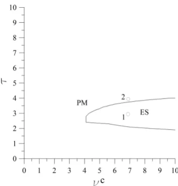
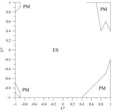
Fig. 2. Parameter domains (τ, νc)admitting equilibrium state (ES) or periodic motion (PM) are illustrated for the single-block model at c=3. Time series and phase portraits corresponding to points 1 and 2 are shown in Fig. 3. The initial function forUis selected such that its values within the interval [−τ,0] are set by Eq. (6) withc=0.

In the present paper, we investigate the behaviour of the trajectories near the stationary solution. In order to study the asymptotic dynamics, we have made certain that all the tran-sients are discarded. As for the fashion in which the delay-differential equations are numerically solved, the initial func-tion forU is selected such that its values within the inter-val [−τ,0] are set by Eq. (6) withc=0 for the single-block model or by Eq. (7) withc1=c2=0 in case of the model

with two blocks.

The results are obtained by varying the control parameters candτ for the model with a single block and the parameter set (c1,c2,τ1,τ2)for the setup involving two blocks. The

observed forms of behaviour are characterised by calculating the Fourier power spectrum and the largest Lyapunov expo-nent. The latter’s value has been obtained by the methods of Wolf et al. (1985) and Rosenstein et al. (1993), with the use of two distinct algorithms aimed at providing additional ver-ification of the results.

4 Model with one block

We first consider the single-block model (6), for which we adoptν=0.1, consistent with (De Sousa Vieira, 1999). The analysis shows that, without the introducedcandτ,and un-der the different values of parameterνc, the original model displays just oscillatory behaviour of various amplitudes. If only the parametercis introduced, under the variation ofνc the behaviour of the model does not change, except for the very low valuesνc<10−8, when the motion of the block settles at the stationary solution.

Fig. 3. Temporal behaviour of variableU˙ and corresponding phase portraits for: (a) equilibrium state (point 1 from Fig. 2; νc=7, τ=3, c=3) and (b) periodic behaviour (point 2 from Fig. 2; νc=7,τ=4,c=3). The phase portrait in (b) is obtained having eliminated the transients.

Next we consider the effects of including the time delayτ in the friction term. If the value of the friction strength pa-rameter is kept atc=1, there is no change in the behaviour of the model. This is expected, since the friction remains the same (Burridge and Knopoff, 1967; Carlson and Langer, 1989). However, if we vary the value ofc, time delay may cause an oscillation death, the effect which has previously been investigated in (Yamaguchi and Shimizu, 1984; Aron-son et al., 1990; Reddy et al., 1998). In particular, asτ is increased, the system undergoes a transition from equilib-rium state to periodic motion and back to equilibequilib-rium state. This feature could have significant practical implications. In an earthquake analogy, the occurrence of oscillation death indicates that the increase of time delay could suppress the seismic activity, and, consequently, the onset of earthquakes. Figure 2 is intended as an illustration of the (τ, νc) param-eter domains admitting equilibrium or periodic motion for the single-block model. In the particular instance, friction strength is set toc=3. Figure 3 shows the time series and phase portraits corresponding to the equilibrium state (sta-tionary solution) and oscillations, observed at the respective points 1 and 2 from Fig. 2. Note that qualitatively similar results are obtained if time delay is held constant, while pa-rametercis varied.

(5)

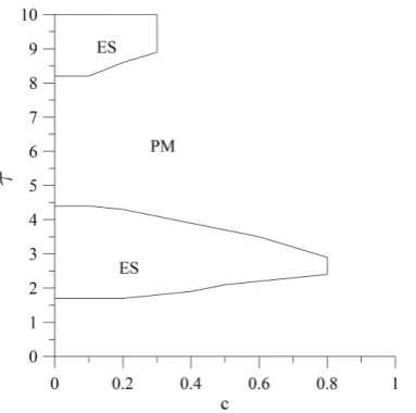
Fig. 4. Parameter domains (τ, c)admitting equilibrium state (ES) or periodic motion (PM) atνc=1. Diagram refers to the single-block model, whereby the 0.1 step size is adopted for bothcandτ.

5 Model with two blocks

The analysis similar to that for the single-block model has been carried out for the setup with two blocks represented by the system (7). In all the examined cases, we fixk1=k2= k=1 as in De Sousa Vieira (1999). Note that the original model, with friction strength parameterc1=c2=1, as in De

Sousa Vieira (1999), and without time delays, exhibits only the periodic motion. We first consider the effects induced by c1andc2, without introducing the delays. The quasiperiodic

motion is obtained under the variation of bothc1andc2while

maintainingνc₁=ν₂c=1. It is found that the model exhibits the limit cycle oscillations only forc1=c2.

Next, if one introducesτ1 andτ2 and assumes

homoge-neous friction strengthc1=c2, the model exhibits

quasiperi-odic motion for all the considered parameter values, except in the caseτ1=τ2(when the motion is periodic). An instance

of quasiperiodic motion for the parameter setτ1=4,τ2=5, c1=c2=2, and νc₁=ν₂c=1 is displayed in Fig. 5. The

phase portrait is plotted in terms ofU˙1vs.U1−U₁e, because

the considered system (7) is nonautonomous, and our goal is to analyse the motion of two blocks in the vicinity of the stationary solution, which is explicitly time-dependent. The corresponding phase portrait in the (_U˙

2,U2−U₂e)plane is not

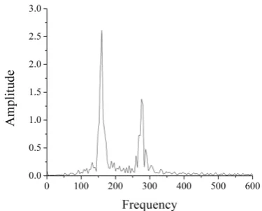
shown, since the attractors of the second block are analogous to those of the first one, as implied in De Sousa Vieira (1999). Two peaks in the Fourier power spectrum (Fig. 6a) and ap-proximately zero value of the maximal Lyapunov exponent (Fig. 6b) obtained for the time series in Fig. 5 confirm that the given motion is indeed quasiperiodic.

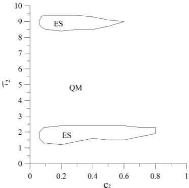
Next we consider the following setup: the first block is held at the equilibrium state (stationary solution) for the un-coupled case,c1=0.1 andτ1=3.0 (see Fig. 2), whereasc2

Fig. 5. Temporal evolution of variableU˙1(a) and corresponding phase portrait (b) forτ1=4,τ2=5, c1=c2=2,k1=k2=k=1 andν₁c=νc₂=1 (quasiperiodic motion).

Fig. 6. Fourier power spectrum (a) and maximal Lyapunov

expo-nent (b) for time series in Fig. 5: (a) Two peaks in the power spec-trum indicate the appearance of quasiperiodic motion. (b) The max-imal Lyapunov exponent converges approximately toλ≈0. Note that in (b) timetis expressed in the units of iteration steps.

andτ2for the second block are varied. From the results

in-dicated in Fig. 7 one reads that the model mainly exhibits quasiperiodic motion, except for the two rather small regions admitting the equilibrium state. The latter scenario occurs only for the low values of the friction strength parameter (c2<1). Note that the limit cycle oscillations (periodic

solu-tions) appear only as a transient feature, resembling the weak quasiperiodic motion.

On the other hand, if (c1,τ1)are selected such that the

first block would show oscillatory behaviour in the uncou-pled case (see Fig. 4), under the variation ofc2 andτ2 the

(6)

Fig. 7. Parameter domains (τ2, c2)admitting periodic motion (PM) or quasiperiodic motion (QM) of the second block.c1=0.1 and

τ1=3.0 are fixed so that the first block lies in the equilibrium state. Diagram is constructed for the 0.1 step size for bothc2 and τ2. Other parameter values are as in Fig. 5. The initial function forU is selected such that its values within the interval [−τ,0] are set by Eq. (7) withc1=c2=0.

In both cases, the obtained values of maximal Lyapunov exponent are positive and of the same order of magnitude, λmax=0.0016 and 0.0019, respectively.

Note that the problem concerning the algorithm appropri-ate for calculating the maximal Lyapunov exponent in case of a transient chaos-like behaviour is still tentative and con-sidered unresolved. In principle, the issue of qualifying cer-tain transient motion as transient chaos should be treated by determining the finite-time Lyapunov exponent (Stefa´nski et al., 2010). In the present paper, by using the methods of Wolf et al. (1985) and Rosenstein et al. (1993) we determined the Lyapunov exponent for the time series showing comparably large transients, whereby the standard procedures are com-plemented by performing additional averaging over a set of different initial conditions (Fig. 12). One notes that the ap-proximately stationary values of the exponents are reached on the time scale significantly smaller than the length of the transient and that the values obtained for different initial con-ditions are quite similar. In particular, for all the examined cases, maximal Lyapunov exponents converge well to posi-tive values (Fig. 12) of the same order of magnitude (10−3). The last stage of our analysis is focused on the issue of how selecting different initial conditions may affect the be-haviour of the model with two blocks. Assuming the homo-geneous initial conditions near the stationary solution (U˙₁o=

˙

U₂0= ˙U0, U₁0=U₂0=U0), we recover either the equilib-rium state or periodic motion, cf. Fig. 13. In this case, quasiperiodic motion is not observed, since the initial con-ditions are chosen near the stationary solution. As apparent from Fig. 13, one is able to clearly distinguish between the

Fig. 8. Parameter domains (τ2, c2)admitting equilibrium state (grey dots), periodic motion (black dots) and quasiperiodic motion (white area), for the fixed parametersc1=0.2,τ1=0.5. The latter values would warrant oscillatory motion for the first block in the uncoupled case. The diagram is constructed for the step size 0.1 for bothc2and

τ2. The remaining parameters are the same as in Fig. 5.

domains supporting either of the two states, which may effec-tively provide an indication on the respective basins of attrac-tion. This also implies that there possibly exists some distant limit cycle attractor which could not be captured by the anal-ysis confined to the vicinity of the unstable stationary solu-tion. Moreover, the obtained results suggest that the system is fairly sensitive to perturbations, meaning that even the small stress changes could induce motion along the fault, and, con-sequently, the onset of earthquakes. One should emphasise that the sensitivity of the block motion on initial conditions was already observed in the work of Szkutnik et al. (2003). In particular, the analysis there has shown that the character of the motion for the three-block model within a certain param-eter range depends on the initial conditions. In other words, changing only the initial position of one of the blocks may induce transition from quasiperiodic and non-synchronized motion to the periodic solution where the two lateral blocks are synchronized.

6 Discussion and conclusion

(7)

Fig. 9. Temporal evolution of variableU˙1(b) and corresponding phase portrait (c) forc1=0.2,τ1=0.5c2=0.2 andτ2=3. In the uncou-pled case, (c1,τ1) would warrant the oscillatory motion of the first block, whereas (c2,τ2) would hold the other block at the equilibrium. The remaining parameter values are:υ₁c=υ₂c=k1=k2=k=1. The time series over a long simulation period is shown in (a), where the chaos-like region is marked with the rectangle. It is apparent that the system eventually converges to quasiperiodic behavior.

Fig. 10. Fourier power spectrum for the time series in Fig. 9. The

continuous broadband noise indicates relatively weak chaotic be-haviour of the system.

co-effect ofcandτ may induce the transition from periodic motion to equilibrium state, cf. Fig. 2, which is consistent with the delay-induced oscillation death. This phenomenon could have significant implications for the real earthquake dynamics, since it indicates the possibility that, under the certain conditions in the Earth’s crust, motion along the fault could be suppressed, or reduced to aseismic creeping. In the model with two blocks, the coaction ofc1,c2,τ1andτ2may

give rise to the transition from periodic to quasiperiodic mo-tion. From Figs. 7 and 8 one reads that such a transition

Fig. 11. Calculation of maximal Lyapunov exponent for the time

series in Fig. 9. (a) indicates the valueλmax=0.0016, obtained by the method of (Wolf et al., 1985). The method of of (Rosenstein et al., 1993), illustrated in (b), impliesλmax≈0.0019. Note that in (a) timet is expressed in the units of iteration steps. In (b), effective expansion rateS(1n) represents the average of the logarithm of Di(1n), defined as the average distance of all nearby trajectories to the reference trajectory as a function of the relative time1n. The slope of dashed lines indicating the predominant slope ofS(1n) in dependence on1ndtpresents a robust estimate for the maximal Lyapunov exponent. The results are determined for 1000 reference points and neighbouring distanceε=0.1–0.15. The obtained values of maximal Lyapunov exponent are of the same order of magnitude.

(8)

Fig. 12. Calculation of maximal Lyapunov exponent by

perform-ing additional averagperform-ing over a set of different initial conditions, whereby U₁0, U₂0,U˙₁0,U˙₂0 belong to the respective ranges U₁0∈ [0,0.003], U₂0∈ [0,0.05],U˙₁0∈ [0,0.003], U₂0∈ [0,0.07]. The re-sults have been obtained by the method of Wolf et al. (1985). Max-imal Lyapunov exponents converge well to positive values of the order 10−3, the same as in Fig. 11. Note that timetis expressed in the units of iteration steps.

layer thickness, indicating the change in friction coefficient µfor more than two times. It should also be stressed that for the model with two blocks, transient chaos-like behaviour is observed. It should be noted that the results of the con-ducted research set a solid base for the further investigation of complex dynamics of the presented models, including the global dynamical behaviour (far from the stationary solution) with heterogeneous initial conditions and different values of spring constants.

Appendix A

Starting off from the system (7):

¨

U1=k1(U2−U1)−U1− c1 1+U˙1(t−τ1)

ν₁c +νt

¨

U2=k2(U1−U2)−U2− c2 1+U˙2(t−τ2)

ν₂c

+νt, (A1)

and setting U˙1= ˙U2=ν, U¨1= ¨U2=0, under the

homo-geneity assumptionk1=k2=kone arrives at:

0=(U2−U1)−U1− c1ν₁c ν₁c+ν+νt

0=(U1−U2)−U2− c2ν₂c

ν₂c+ν+νt. (A2)

Fig. 13. Domains of initial conditions (U˙₁0= ˙U₂0= ˙U0, U₁0=

U₂0=U0) admitting equilibrium state (ES) or periodic motion (PM). The results are obtained for the parameter setc1=c2=0.1,

τ1=τ2=3.0. Diagram is constructed for the step size equal of 0.1 for both U˙0 and U0. The remaining parameter values are: ν₁c=ν₂c=1,k1=k2=k=1.

Adding the equations in system (A2) results in the expres-sion:

−(U1+U2)=

_c

1ν1c ν₁c+ν+

c2ν2c ν₂c+ν

−2νt. (A3)

On the other hand, by subtracting the second equation from the first one in Eq. (A2), the following relation is ob-tained:

3(U2−U1)+

_c

2ν2c ν₂c+ν −

c1ν1c νc₁+ν

=0, (A4)

from where we get: U1=U2+

1 3

_c

2ν2c ν₂c+ν−

c1ν1c ν₁c+ν

U2=U1+

1 3

_c

1ν₁c νc₁+ν−

c2ν₂c ν₂c+ν

. (A5)

After substituting Eq. (A5) into Eq. (A3), the equations for the equilibrium of the system (A1) finally become

U₁e= −1

3

2 c1ν c 1 ν₁c+ν+

c2ν₂c ν₂c+ν

+νt

U₂e= −1

3

2 c2ν c 2 ν₂c+ν+

c1ν1c ν₁c+ν

+νt (A6)

(9)

Acknowledgements. This research has been supported by the Serbian Ministry of Education, Science and Technological Devel-opment, Contracts No. 176016, 171017 and 171015.

Edited by: J. M. Redondo

Reviewed by: two anonymous referees

References

Aronson, D., Ermentout, G., and Kopell, N.: Amplitude response of coupled oscillators, Physica D, 41, 403–449, 1990.

Bak, P. and Tang, C.: Earthquakes as a self-organized critical phe-nomenon, J. Geophys. Res., 94, 15635–15637, 1989.

Behnsen, J. and Faulkner, D. R.: The effect of mineralogy and ef-fective normal stress on frictional strength of sheet silicates, J. Struct. Geol., 30, 1–13, 2012.

Beltrami, H. and Mareshal, J.: Strange seismic attractor?, Pure Appl. Geophys., 141, 71–81, 1993.

Buri´c, N. and Todorovi´c, D.: Dynamics of delay-differential equa-tions modeling immunology of tumor growth, Chaos Soliton. Fract., 13, 645–655, 2002.

Burridge, R. and Knopoff, L.: Model and theoretical seismicity, B. Seismol. Soc. Am., 57, 341–371, 1967.

Byerlee, J. D.: Frictional characteristics of granite under high con-fining pressure, J. Geophys. Res., 72, 36390–36448, 1967. Byerlee, J. D. and Summers, R.: A note on the effect of fault gouge

thickness on fault stability, Int. J. Rock Mech. Mining Sci. Ge-omech. Abstr., 13, 35–36, 1976.

Carlson, J. M. and Langer, J. S.: Mechanical model of an earthquake fault, Phys. Rev. A, 40, 6470–6484, 1989.

Das, S., Boatwright, J., and Scholz, C. H. (Eds.): Earthquake source mechanics, Am. Geophys. Union Monogr., Washington DC, 1986.

De Sousa Vieira, M.: Chaos in a simple spring-block system, Phys. Lett. A, 198, 407–414, 1995.

De Sousa Vieira, M.: Chaos and synchronized chaos in an earth-quake model, Phys. Rev. Lett., 82, 201–204, 1999.

Dieterich, J. H.: Modeling of rock friction: 1. Experimental results and constitutive equations, J. Geophys. Res., 84, 2161–2168, 1979.

Engelder, J. T., Logan, J. M., and Handin, J.: The sliding character-istics of sandstone on quartz fault-gouge, Pure Appl. Geophys., 113, 69–86, 1975.

Erickson, B., Birnir, B., and Lavallee, D.: A model for aperiodicity in earthquakes, Nonlinear Proc. Geoph., 15, 1–12, 2008. Gopalsamy, K. and Leung, I.: Delay induced periodicity in a neural

netlet of excitation and inhibition, Physica D, 89, 395–426, 1996. Horowitz, F. G. and Ruina, A.: Slip patterns in a spatially

homoge-neous fault model, J. Geophys. Res., 94, 10279–10298, 1989. Langer, J. S., Carlson, J. M., Myers, C. R., and Shaw, B. E.: Slip

complexity in dynamics models of earthquake faults, Proc. Natl. Acad. Sci. USA, 93, 3825–3829, 1996.

Marone, C.: The effect of loading rate on static friction and the rate of fault healing during the earthquake cycle, Nature, 391, 69–72, 1998.

Marone, C. and Scholz, C. H.: The depth of seismic faulting and the upper transition from stable to unstable slip regimes, Geophys. Res. Lett., 15, 621–624, 1988.

Marone, C., Raleigh, C. B., and Scholz, C. H.: Frictional behaviour and constitutive modeling of simulated fault gouge, J. Geophys. Res., 95, 7007–7025, 1990.

Marsan, D., Bean, C. J., Steacy, S., and McCloskey, J.: Observa-tion of diffusion processes in earthquake populaObserva-tions and impli-cations for the predictability of seismicity systems, J. Geophys. Res., 105, 28081–28094, 2000.

Mizoguchi, K., Fukuyama, E., Kitamura, K., Takahasi, M., Masuda, K., and Omura, K.: Depth dependent strength of the fault gouge at the Atotsugawa fault, central Japan: a possible mechanism for its creeping motion, Phys. Earth Planet. In., 161, 115–125, 2007. Morrow, C. A., Moore, D. E., and Lockner, D. A.: The effect of min-eral bond strength and adsorbed water on fault gouge frictional strength, Geophys. Res. Lett., 27, 815–818, 2000.

Okubo, P. G. and Aki, K.: Fractal geometry in the San Andreas fault system, J. Geophys. Res., 92, 345–355, 1987.

Pomeau, Y. and Le Berre, M.: Critical speed-up vs critical slow-down: a new kind of relaxation oscillation with application to stick-slip phenomena, arXiv: 1107.3331v1, 2011.

Reddy, D., Sen, A., and Johnston, G.: Time delay induced death in coupled limit cycle oscillators, Phys. Rev. Lett., 80, 5109–5112, 1998.

Rice, J. R.: Constitutive relations for fault slip and earthquake insta-bilities, Pure Appl. Geophys., 121, 443–475, 1983.

Rice, J. R. and Ruina, A. L.: Stability of steady frictional slipping, J. Appl. Mech. 50, 343–349, 1983.

Rosenstein, M. T., Collins, J. J., and De Luca, C. J.: A practical method for calculating largest Lyapunov exponents from small data sets, Physica D, 65, 117–134, 1993.

Ruina, A.: Slip instability and state variable friction laws, J. Geo-phys. Res., 88, 10359–10370, 1983.

Scholz, C. H., Wyss, M., and Smith, S. W.: Seismic and aseismic slip on the San Andreas fault, J. Geophys. Res., 74, 2049–2069, 1969.

Sibson, R. H.: Fault rocks and fault mechanisms, J. Geol. Soc. Lon-don, 133, 191–213, 1977.

Smith, H.: An introduction to delay differential equations with ap-plications to the life sciences, Vol. 57, Texts in applied mathe-matics, Springer, 172 pp., 2011.

Stefa´nski, K., Buszko, K., and Piecyk, K.: Transient chaos measure-ments using finite-time Lyapunov exponents, Chaos, 20, 033117-1-13, 2010.

Szkutnik, J., Kawecka-Magiera, B., and Kulakowski, K.: History-dependent synchronization in the Burridge-Knopoff model, Tri-bology S, 43, 529–536, 2003.

Turcotte, D. L., Newman, W. I., and Gabrielov, A.: A statisti-cal physics approach to earthquakes, in Geocomplexity and the Physics of Earthquakes, Geophysical monograph 120, edited by: Rundle, J. B., Turcotte, D. L., and Klein, W., American Geophys-ical Union, Washington, USA, 83–96, 2000.

Wolf, A., Swift, J., Swinney, H., and Vastano, J.: Determining Lya-punov exponents from a time series, Physica D, 16, 285–317, 1985.