Variation in emission metrics due to variation in CO2 and temperature impulse response functions

(1)

Earth Syst. Dynam., 4, 267–286, 2013 www.earth-syst-dynam.net/4/267/2013/ doi:10.5194/esd-4-267-2013

EGU Journal Logos (RGB)

Advances in

Geosciences

Open Access

Natural Hazards

and Earth System

Sciences

Open Access

Annales

Geophysicae

Open Access

Nonlinear Processes

in Geophysics

Open Access

Atmospheric

Chemistry

and Physics

Open Access

Atmospheric

Chemistry

and Physics

Open Access

Discussions

Atmospheric

Measurement

Techniques

Open Access

Atmospheric

Measurement

Techniques

Open Access

Discussions

Biogeosciences

Open Access Open Access

Biogeosciences

Discussions

Climate

of the Past

Climate

of the Past

Discussions

Earth System

Dynamics

Earth System

Dynamics

Discussions

Geoscientific

Instrumentation

Methods and

Data Systems

Open Access

Geoscientific

Instrumentation

Methods and

Data Systems

Open Access

Discussions

Geoscientific

Model Development

Geoscientific

Model Development

Discussions

Hydrology and

Earth System

Sciences

Open Access

Hydrology and

Earth System

Sciences

Open Access

Discussions

Ocean Science

Discussions

Solid Earth

Discussions

The Cryosphere

Discussions

Natural Hazards

and Earth System

Sciences

Open Access

Discussions

Variation in emission metrics due to variation in CO

2

and temperature impulse response functions

D. J. L. Olivi´e1,2and G. P. Peters1

1_{Center for International and Environmental Climate Research – Oslo (CICERO), Oslo, Norway} 2_{Department of Geosciences, University of Oslo, Oslo, Norway}

Correspondence to: D. J. L. Olivi´e ([email protected])

Received: 30 July 2012 – Published in Earth Syst. Dynam. Discuss.: 3 September 2012 Revised: 8 May 2013 – Accepted: 30 June 2013 – Published: 8 August 2013

Abstract. Emission metrics are used to compare the climate

effect of the emission of different species, such as carbon dioxide (CO2) and methane (CH4). The most common

met-rics use linear impulse response functions (IRFs) derived from a single more complex model. There is currently lit-tle understanding on how IRFs vary across models, and how the model variation propagates into the metric values.

In this study, we first derive CO2 and temperature IRFs

for a large number of complex models participating in dif-ferent intercomparison exercises, synthesizing the results in distributions representing the variety in behaviour. The de-rived IRF distributions differ considerably, which is partially related to differences among the underlying models, and par-tially to the specificity of the scenarios used (experimental setup).

In a second part of the study, we investigate how differ-ences among the IRFs impact the estimates of global warm-ing potential (GWP), global temperature change potential (GTP) and integrated global temperature change potential (iGTP) for time horizons between 20 and 500 yr.

Within each derived CO2 IRF distribution, underlying

model differences give similar spreads on the metrics in the range of−20 to+40 % (5–95 % spread), and these spreads are similar among the three metrics.

GTP and iGTP metrics are also impacted by variation in the temperature IRF. For GTP, this impact depends strongly on the lifetime of the species and the time horizon. The GTP of black carbon shows spreads of up to−60 to+80 % for time horizons to 100 yr, and even larger spreads for longer time horizons. For CH4the impact from variation in the

tem-perature IRF is still large, but it becomes smaller for longer-lived species. The impact from variation in the temperature

IRF on iGTP is small and falls within a range of±10 % for all species and time horizons considered here.

We have used the available data to estimate the IRFs, but we suggest the use of tailored intercomparison projects spe-cific for IRFs in emission metrics. Intercomparison projects are an effective means to derive an IRF and its model spread for use in metrics, but more detailed analysis is required to explore a wider range of uncertainties. Further work can re-veal which parameters in each IRF lead to the largest un-certainties, and this information may be used to reduce the uncertainty in metric values.

1 Introduction

Emission metrics are routinely used as a simple means of comparing the climate impact of the emission of various species. The most common emission metric is the global warming potential (GWP), but the global temperature change potential (GTP) has received considerable attention more re-cently (Fuglestvedt et al., 2003; Aamaas et al., 2013). Both these metrics compare the climate impact of the pulse sion of a certain species with the impact of the pulse emis-sion of the same amount of carbon dioxide (CO2). The GWP

(2)

268 D. J. L. Olivi´e and G. P. Peters: Variation in emission metrics

similar, with one quantifying the energy added to the sys-tem (GWP), and the other quantifying the energy lost (iGTP) (Peters et al., 2011; Azar and Johansson, 2012).

Together with the climate impact to be evaluated, the time horizon is an important quantity affecting the metric values (Fuglestvedt et al., 2003; Aamaas et al., 2013). Frequently used time horizons are 20, 100, and 500 yr for GWP, and 20, 50, and 100 yr for GTP (Fuglestvedt et al., 2003, 2010; Shine et al., 2005, 2007). A GWP with a 100 yr time horizon is by far the most common emission metric due to its application in climate policies such as the Kyoto Protocol.

Emission metrics generally condense the complex be-haviour of the climate response into a simple set of equa-tions. In general, the behaviour of a dynamical system can be described to a large extent by its response to a pulse pertur-bation, and this response is called the impulse response func-tion (IRF). In the case of a linear system, the IRF completely characterizes the dynamics of the system, and the response to a general perturbation can be expressed by the time convolu-tion of the IRF with the general perturbaconvolu-tion (Wigley, 1991). In the context of emission metrics, IRFs are used in two ways. Firstly, they are used to characterize the atmospheric concentration of a given species following a pulse emission. Most species will show a single exponential decay, but the atmospheric CO2concentration following a pulse emission

is more complex (Joos et al., 2013). Secondly, IRFs are also used to characterize the global temperature change induced by a pulse radiative forcing (Hasselmann et al., 1993; Sausen and Schumann, 2000). If one additionally linearizes the ex-pression for the radiative forcing to obtain the radiative effi-ciency (Aamaas et al., 2013), one obtains a simple and useful description of the atmospheric response to the emissions of radiatively active species through a simple combination of the radiative efficiency and IRFs.

By using IRFs in the expression of emission metrics, the climate impact is explicitly decoupled into three indepen-dent parts: (i) the additional radiative forcing for a marginal increase in burden (radiative efficiency); (ii) the impact of an emission on the atmospheric burden; and, (iii) the im-pact of radiative forcing on the global-mean temperature for temperature-based metrics. In a coupled system, temperature changes (which might be caused by a CO2perturbation) will

modify the absorption of CO2 in the ocean directly due to

the temperature dependency of the CO2 solubility, but also

by changes in the ocean circulation patterns, and by the bio-sphere, directly through increased respiration and photosyn-thesis or indirectly by changing precipitation (Joos et al., 1996; Friedlingstein et al., 2006; Archer et al., 2009). Many of these processes are non-linear and path dependent, and thus the IRFs are only valid for specific conditions, such as temperature (determining the CO2solubility in the ocean) or

reference tracer concentration. In addition, the radiative ef-ficiency of a specific species might also depend on its con-centration and on the concon-centration of species with which there might be a spectral overlap (Tanaka et al., 2009; Gillett

and Matthews, 2010; Reisinger et al., 2011). In non-linear systems (for example increased photosynthesis by higher at-mospheric CO2concentrations – fertilization effect), the IRF

will be influenced by the size and timing of the pulse (Hooss et al., 2001; Eby et al., 2009; Joos et al., 2013).

In principle, every system behaves linearly for small per-turbations, and as metrics are defined as a tool to compare the impact of small emission changes (1 kg), there is a strong interest in this linear domain. Below a certain threshold, the behaviour of the IRFs will be rather independent of the size of the pulse. For CO2pulse sizes below 100 Gt[C], the IRF is

found to be linear, but the IRF still depends on the timing and the emissions pathway (Joos et al., 2013). The non-linearities caused by the timing and pathway of emissions partially can-cel (Caldeira and Kasting, 1993), though regular updates of IRFs are needed (Reisinger et al., 2011; Joos et al., 2013).

IRFs are nevertheless useful and efficient means to de-scribe the behaviour of more complex systems (or models). They allow fast and sufficiently robust metric calculations, and give the possibility to efficiently estimate the impact of many different scenarios, as long as one remains in a linear regime. In recent times, the GWP and GTP have used a CO2

IRF (IRFCO2) based on an updated version of the Bern

cou-pled climate–carbon cycle model (CC-model) described in Plattner et al. (2008, Bern2.5CC), and the temperature IRF (IRFT) from Boucher and Reddy (2008) based on a simu-lation with the UKMO-HadCM3 atmosphere–ocean general circulation model (AOGCM). As these IRFs are based on the behaviour of only one parent model, one should regard their application with care as they may be outliers. It is thus rele-vant to assess how IRFs (and consequently metric values) can differ among models. In recent years, many idealized simula-tions with CC-models and AOGCMs have become available in intercomparison exercises, which can be used to derive IRFCO2 or IRFT. The behaviour of these models differs

con-siderably, and one of the aims of this study is to investigate how this is translated into variations in the IRFs. We will also use these derived IRFs to calculate GWP, GTP, and iGTP val-ues, and quantify how they are influenced by variation in the IRFs.

This work builds on former work where IRFT is estimated based on AOGCM simulations performed within the CMIP3 project (Olivi´e et al., 2012). Here, we extend the estima-tion of IRFT to CMIP5 data (Taylor et al., 2012), and use the method additionally to estimate IRFCO2 from recent

in-tercomparison exercises (C4MIP, Friedlingstein et al., 2006; LTMIP, Archer et al., 2009, and Joos et al., 2013). Due to the considerable number of models participating, we can en-lighten the variation of IRFs among models, and estimate the impact of variation in IRFCO2 and IRFT on metric values.

Uncertainties in the lifetime of the non-CO2species and in

(3)

D. J. L. Olivi´e and G. P. Peters: Variation in emission metrics 269

not necessarily represents the scientific uncertainty (Knutti, 2010; Reisinger et al., 2010). Our work is comparable with Reisinger et al. (2010), who presented uncertainty estimates for emission metrics of CO2and CH4using a simple climate

model calibrated on CMIP3 AOGCM results and C4MIP CC-model results (partially using results from OCMIP2). With respect to their study, we study more species (black carbon (BC), methane (CH4), nitrous oxide (N2O) and sulfur

hex-afluoride (SF6)), and use data from more intercomparison

exercises (LTMIP, CMIP5, and Joos et al., 2013).

The structure of the paper is as follows. In Sect. 2, we de-scribe emission metrics and IRFs. In Sect. 3, we dede-scribe the data and method we use to derive IRFs. In Sect. 4, we present the derived IRFs, and the impact of variation in IRFs on emis-sion metrics. In Sect. 5, we present our concluemis-sions.

2 Emission metrics and IRFs

2.1 IRFs

In the context of emission metrics, IRFs are used as a con-densed way to describe the evolution of the atmospheric bur-den of species after their emission, or the evolution of the global-mean temperature in response to a radiative forcing.

2.1.1 Burden IRFs

The evolution of the atmospheric burden after the pulse emis-sion of 1 kg of a speciesXis often written as a sum of de-caying exponential functions (modes),

IRFX(t )= n−1 X

i=0

aiexp

−t τi

, (1)

with n−1 X

i=0

ai=1. (2)

The atmospheric burdenBX(t )in response to any emission scenarioEX(t )can be written as the convolution integral

BX(t )=(EX⊗IRFX)(t )

≡

t

Z

−∞

EX(t0)IRFX(t−t0)dt0. (3)

For most species one usually limits the expression to one mode, where the uniqueτ in Eq. (1) represents the pertur-bation lifetime of the species (Prather, 2007). In this study, we consider species with a wide range of lifetimes to cap-ture the different dynamics: BC, CH4, N2O, and SF6. BC

has a lifetime of around a week, but it may vary depend-ing on the location and timdepend-ing of the emissions, while CH4,

N2O, and SF6have more stable lifetimes of around 12, 114,

and 3200 yr, respectively (see Table 1).

We take into account the impact of CH4and N2O on their

own lifetimes (Seinfeld and Pandis, 2006; Prather, 2007). Emissions of CH4also lead to the formation of tropospheric

ozone and stratospheric water vapour (their radiative impact is included in the radiative efficiency of CH4). The radiative

forcing from CO2 produced in the oxidation of CH4is not

taken into account, as this CO2is often already accounted for

in the CO2emission inventories (for its impact, see Boucher

et al., 2009). One should also be aware of the fact that tro-pospheric OH concentrations which determine the loss rate of CH4are estimated to have uncertainties of around±15 %

(Reisinger et al., 2011).

The perturbation lifetime of CO2is more complex. A part

of a pulse emission disappears rapidly from the atmosphere on a timescale of 1 to 10 yr, while a substantial part remains in the atmosphere for a much longer time (Archer et al., 1997, 2009). One mode is insufficient to describe the atmospheric CO2 burden evolution after a pulse emission (Joos et al.,

1996; Forster et al., 2007; Archer et al., 2009). A satisfac-tory description for the evolution of CO2used in Forster et al.

(2007) is an expression with four modes (n=4 in Eq. 1), and the corresponding values ofai andτi are given in the upper row of Table 3. Notice thatτ0= ∞, indicating that 21.7 % of

the emission is assumed to stay perpetually in the atmosphere (a0=0.217).

If one additionally assumes that the RF is a linear function of the atmospheric burden, then the evolution of the RF as a function of time can be expressed by a simple multiplica-tion of the radiative efficiency and the IRF (Aamaas et al., 2013). In general linearity does not hold for CO2, CH4, or

N2O where the RF shows a non-linear dependence on their

burden – moreover N2O and CH4 have a spectral overlap

(Ramaswamy et al., 2001, Table 6.2). However, a linear ap-proximation can be used when assuming a marginal perturba-tion around a well-defined reference state. Approximate val-ues for the radiative efficiency of different species are given in Table 1. The radiative efficiency of CO2(see Table 1) is

based on the radiative forcing expression for CO2 in

Ra-maswamy et al. (2001, Table 6.2), assuming a background mixing ratio of 378 ppm (Forster et al., 2007, Sect. 2.10.2 and Table 2.14).

2.1.2 Temperature IRF

IRFs are also used to express the temperature evolution in re-sponse to a specified radiative forcing. The expected global-mean temperature change, T (t ), due to a radiative forcing can be approximately described by a convolution integral of the radiative forcing, RF(t ), with the temperature IRF, IRFT(t ):

T (t )=(RF⊗IRFT)(t )≡

t

Z

−∞

(4)

Table 1. Lifetime and radiative efficiency of BC, CH₄, CO₂, N₂O, and SF₆(see Forster et al., 2007, and Fuglestvedt et al., 2010). For the lifetime of CO2, see Table 3.

BC CH₄ CO₂ N₂O SF₆

τ (yr) 0.02 12 – 114 3200

AX (W m−2kg−1) 1.96×10−9 1.82×10−13 1.81×10−15 3.88×10−13 2.00×10−11

The IRFT is often described as a sum of decaying exponen-tial functions,

IRFT(t )= n

X

i=1

fi

τi exp−t

τi

. (5)

This function describes the evolution of the global-mean temperature change after aδ-pulse radiative forcing (the in-tegrated amount of forcing from aδ-pulse imposed on the system is comparable to a forcing of 1 W m−2during 1 yr). For a RF step scenario that jumps att=0 from 0 to 1 W m−2 and remains constant at that value fort >0, one finds, using Eqs. (4) and (5), that the temperature evolutionT (t )can be written as

T (t )=

n

X

i=1

fi

1−exp−t

τi

. (6)

This shows that the sum of the fi in IRFT can be inter-preted as the climate sensitivity, i.e.λ=

n

P

i=1

fi (takingt→

∞in Eq. 6). The climate sensitivity is here defined as the change in equilibrium global-mean temperature per unit forc-ing (Hansen et al., 2005; Hansen and Sato, 2012).

In the literature, one finds IRFT expressions withn=1 (Hasselmann et al., 1993; Shine et al., 2005),n=2 (Hooss et al., 2001; Boucher and Reddy, 2008), and n=3 (Li and Jarvis, 2009). Using two time constants describes the AOGCM temperature evolution response to a RF reasonably well (Boucher and Reddy, 2008; Li and Jarvis, 2009; Olivié and Stuber, 2010; Olivié et al., 2012), while one time con-stant is inadequate for most applications (Shine et al., 2005; Gillett and Matthews, 2010; Olivié et al., 2012). A frequently used expression withn=2 is the one presented in Boucher and Reddy (2008), and the corresponding values offi andτi are given in the upper row of Table 4. For expressions with

n≥2, the first mode represents the fast response of the atmo-sphere, the land surface, and the ocean mixed layer, while the other modes represent the slow response of the deep ocean.

2.2 Emission metrics

Emission metrics are a useful tool to efficiently quantify and compare the impact of the emissions of different species. While emission metrics can also be calculated using more complex models (Wuebbles et al., 1995; Tanaka et al., 2009, 2010; Reisinger et al., 2010; Gillett and Matthews, 2010), we use the IRF approach as described above due to its efficiency, repeatability, and utility in a wide range of applications.

The absolute global warming potential (AGWP) of a species is the time-integrated RF caused by the emission of 1 kg of that species,

AGWPX(H )= H

Z

0

AXIRFX(t )dt , (7)

withHthe time horizon, IRFX(t )the burden IRF (see Eq. 1), andAX the radiative efficiency of speciesX. The radiative efficiency can depend on the background concentration, but we assume a constant background as is common for emission metrics (Joos et al., 2013; Aamaas et al., 2013). The radiative efficiency values we use are given in Table 1. The dimension-less GWP of a species is the AGWP of that species divided by the AGWP of CO2,

GWPX(H )=

AGWPX(H )

AGWPCO2(H )

. (8)

The GWP metric has been used extensively over the last two decades to compare the climate effect of various species.

By combining the burden IRF and the temperature IRF, one can express the global-mean temperature response due to the emission of a species. The absolute global temperature change potential (AGTP) indicates the impact of the emis-sion of 1 kg of a certain species on the global-mean tempera-ture at a certain time,

AGTPX(H )= H

Z

0

AXIRFX(t )IRFT(H−t )dt , (9)

with IRFT(t )the temperature IRF (see Eq. 5). The dimen-sionless GTP of a species is the AGTP of that species divided by the AGTP of CO2,

GTPX(H )=

AGTPX(H ) AGTPCO2(H )

. (10)

The integrated absolute temperature change potential (iAGTP) is the time integral of AGTP,

iAGTPX(H )= H

Z

0

AGTPX(t )dt . (11)

The dimensionless iGTP of a species is the iAGTP of that species divided by the iAGTP of CO2,

iGTPX(H )=

iAGTPX(H )

iAGTPCO2(H )

(5)

D. J. L. Olivi´e and G. P. Peters: Variation in emission metrics 271

3 Method and data

To obtain estimates for IRFCO2 and IRFT, we use results

from more complex models. As we are interested in possible uncertainties in emission metrics, we focus on data from in-tercomparison exercises with different models participating in the same experimental setup.

3.1 Data

Here we describe the data used to derive the IRFs. We will also shortly describe the data on which the reference IRFCO2

(Forster et al., 2007) and IRFT (Boucher and Reddy, 2008) are based. An overview of some of the characteristics of the intercomparison exercises can be found in Table 2.

3.1.1 Forster et al. (2007)

The IRFCO2 which has been used in Forster et al. (2007), is

based on a 1000 yr-long simulation with the Bern CC-model (Plattner et al., 2008, Bern2.5CC). In that simulation, a back-ground CO2mixing ratio of 378 ppm and a pulse emission of

40 Gt[C] were used. We will refer to this data set and IRFCO2

derived from it as J07.

3.1.2 C4MIP

The C4MIP (Coupled Climate–Carbon Cycle Model Inter-comparison Project) experiments have been performed sim-ulating the 1860–2100 period with CC-models (Friedling-stein et al., 2006). For the anthropogenic CO2emissions,

esti-mates based on observed concentrations have been used up to around year 2000 and SRES scenario A2 values for the 21st century (Nakicenovic et al., 2000). The annual emissions increase from∼1 Gt[C] yr−1 in 1900, to∼8 Gt[C] yr−1 in 2000, and∼30 Gt[C] yr−1in 2100.

Eleven CC-models participated in this intercomparison ex-ercise, of which 7 are AOGCMs and 4 are models of in-termediate complexity. These models are BERN-CC, CSM-1, CLIMBER2-LPJ, FRCGC, HadCM3LC, IPSL-CM2C, LLNL, IPSL-CM4-LOOP, MPI, UMD, and Uvic-2.7. A short description of these models can be found in Friedling-stein et al. (2006). Two different experiments were per-formed. In an uncoupled experiment (u) temperature feed-backs on the carbon cycle were not included, while in the coupled experiment (c) temperature feedbacks were in-cluded. All models indicated that a larger fraction of anthro-pogenic CO2stays airborne if temperature feedbacks are

in-cluded.

3.1.3 LTMIP

A second data set we use to derive IRFCO2 is LTMIP

(Long Tail Model Intercomparison Project) (Archer et al., 2009). The aim of this project was to quantify the long-term fate of fossil fuel CO2 emissions in the atmosphere,

ocean, and terrestrial biosphere. The participating groups performed 104yr-long simulations with CC-models, emit-ting CO2 pulses of 1000 Gt[C] and 5000 Gt[C]. The

refer-ence state was an atmospheric mixing ratio of 286 ppm CO2.

Different simulations have been performed, differing by the feedbacks taken into account in the CC-models. We have used the results from the reference simulation with a 1000 Gt[C] pulse emission and no feedbacks – this is a simulation performed by most of the models. These models are CC SED, CLIMBER-2, GENIE8, GENIE16, GEOCYC, LTCM, MESMO, MPI-UW, and UVIC-2.8. A short descrip-tion of these models can be found in Archer et al. (2009) and Cao et al. (2009). With one of these models (UVIC-2.8), Eby et al. (2009) further illustrate that the time required to absorb anthropogenic CO2strongly depends on the total emission

amount.

3.1.4 Joos et al. (2013)

The recent study of Joos et al. (2013) estimated IRFCO2 with

current state-of-the-art CC-models. They performed simu-lations with a length of 1000 yr and an emission pulse of 100 Gt[C]. The reference state was an atmospheric mix-ing ratio of 389 ppm CO2. The 15 models of which we

used data are ACC2, Bern2.5D-LPJ, Bern3D-LPJ, Bern-SAR, CLIMBER-2-LPJmL, DCESS, GENIE, HadGEM2-ES, LOVECLIM1.1, MAGICC6, MESMO1.00, MPI-ESM, NCAR CSM1.4, TOTEM, and UVic2.9. We will refer to this data set as J13. Joos et al. (2013) additionally studied the impact of a CO2pulse emission on the global-mean

temper-ature, sea level, and ocean heat content, and performed a va-riety of sensitivity studies.

3.1.5 Boucher and Reddy (2008)

Boucher and Reddy (2008) present an IRFT, derived from a 1000 yr-long simulation with the UKMO-HadCM3 AOGCM. In this simulation the RF was modified by increas-ing the CO2 concentration by 2 % yr−1up to a quadrupling

(reached after 70 yr), after which the CO2concentration was

kept constant. The IRFT of Boucher and Reddy (2008) con-tains two modes, with time constants of 8.4 and 409.5 yr. The values offi andτi can also be found in the top row of Ta-ble 4. Li and Jarvis (2009) used the same data but a different method to estimate the modes. Using two modes they find very similar values, and using three modes small differences in the integrated IRFT only show up after 500 yr.

3.1.6 CMIP3

(6)

272 D. J. L. Olivi´e and G. P. Peters: Variation in emission metrics

Table 2. Overview of the different data sets used to derive IRF_CO₂ and IRF_T. The number of models used here might be lower than the number of models participating in the intercomparison exercise.

Experimental setup Length Models Release Reference (yr) (#)

J07 Pulse CO₂emission 1000 1 2007 Forster et al. (2007) C4MIP Gradual CO2emission (SRES A2) 140 (240) 11 2006 Friedlingstein et al. (2006)

LTMIP Pulse CO₂emission 10 000 9 2009 Archer et al. (2009) J13 Pulse CO2emission 1000 15 2013 Joos et al. (2013)

BR08 Linear RF increase + stabilization 1000 1 2008 Boucher and Reddy (2008) CMIP3 Linear RF increase + stabilization 70–300 15 2006 Randall et al. (2007) CMIP5 Step RF increase/linear RF increase 140–150 15 2011 Taylor et al. (2012)

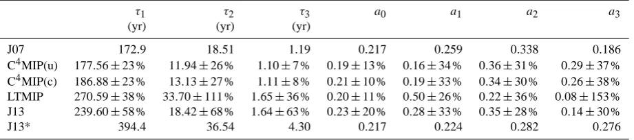
Table 3. Estimates of the parameters in IRFCO2: J07 is the IRFCO2 used in Forster et al. (2007), and C

4_{MIP(u), C}4_{MIP(c), and LTMIP}

are the IRFCO2derived using the corresponding data sets. C

4_{MIP(c) represents an experiment with a temperature feedback, and C}4_MIP(u)

without. J13* refers to the coefficients as derived and published in Joos et al. (2013). In all the IRF_CO₂ isτ0= ∞. The median, and 5- and

95-percentile values are indicated.

τ1 τ2 τ3 a0 a1 a2 a3

(yr) (yr) (yr)

J07 172.9 18.51 1.19 0.217 0.259 0.338 0.186 C4MIP(u) 177.56±23 % 11.94±26 % 1.10±7 % 0.19±13 % 0.16±34 % 0.36±31 % 0.29±37 % C4MIP(c) 186.88±23 % 13.13±27 % 1.11±8 % 0.21±10 % 0.19±33 % 0.34±30 % 0.26±38 % LTMIP 270.59±38 % 33.70±111 % 1.65±36 % 0.20±11 % 0.50±26 % 0.22±36 % 0.08±153 % J13 239.60±58 % 18.42±68 % 1.64±63 % 0.23±20 % 0.28±33 % 0.35±28 % 0.14±30 % J13* 394.4 36.54 4.30 0.217 0.224 0.282 0.276

idealized experiments where the CO2 concentration

in-creases by 1 % yr−1, and is kept constant after 70 yr (doubling of CO2) or after 140 yr (quadrupling of CO2).

These are gradually changing scenarios, and have for most of the AOGCMs a length of 210–290 yr, but less than 100 yr for a few of them. The subset of 15 models we use consists of CGCM3.1(T47), CNRM-CM3, ECHO-G, FGOALS-g1.0, GFDL-CM2.0, GFDL-CM2.1, GISS-EH, GISS-ER, INM-CM3.0, IPSL-CM4, MIROC3.2(hires), MIROC3.2(medres), MRI-CGCM2.3.2, UKMO-HadCM3, and UKMO-HadGEM1. More information on these models can be found in Randall et al. (2007).

For the models used in this intercomparison exercise (ex-cept for CNRM-CM3), also the climate sensitivity λ (see Sect. 2.1.2) has been estimated in Randall et al. (2007, Ta-ble 8.2) based on an experiment where the atmosphere gen-eral circulation models alone were coupled to a mixed layer ocean model (Solomon et al., 2007). In one of the approaches we use the estimated climate sensitivity as an additional con-straint, and we refer to that case as CMIP3*.

3.1.7 CMIP5

From the more recent CMIP5 exercise (Taylor et al., 2012), we use the scenario with an instantaneous qua-drupling of the CO2 concentration, and the one with

a gradual increase in CO2 concentration at a rate of

1 % yr−1 (without stabilization). The length of the simu-lations is 140–150 yr, which is considerably shorter than the experiments in CMIP3. We use the results from 15 models, i.e. CanESM2, CNRM-CM5, CSIRO-Mk3.6.0, GFDL-CM3, GFDL-ESM2G, GFDL-ESM2M, HadGEM2-ES, INM-CM4, IPSL-CM5A-LR, MIROC5, MIROC-ESM, MPI-ESM-LR, MPI-ESM-P, MRI-CGCM3, and NorESM1-M.

3.2 Method

In this section, we explain how we estimate the parameters in the IRFs, how we construct the IRF distributions, and how we calculate the spread in the emission metrics.

3.2.1 Estimating the IRF parameters

For every CC-model and AOGCM in the data sets above, we have estimated the parameters in the IRFs of Eqs. (1) and (5), respectively. We choose to use four modes (n=4) in IRFCO2 (one of which is a constant term as we takeτ0= ∞)

(7)

D. J. L. Olivi´e and G. P. Peters: Variation in emission metrics 273

Table 4. Estimates of the parameters in IRF_T: BR08 is the IRF_T used in Boucher and Reddy (2008), and CMIP3, CMIP3*, and CMIP5 are the IRFT derived using CMIP3 and CMIP5 data. The CMIP3 IRFT is based on AOGCM experiments alone, while the CMIP3* IRFT additionally includes the independently estimated climate sensitivities. The median, and 5- and 95-percentile values are indicated.

τ1 τ2 f1 f2

(yr) (yr) (K W−1m2) (K W−1m2) BR08 8.4 409.5 0.631 0.429 CMIP3 7.15±35 % 105.55±38 % 0.48±30 % 0.20±52 % CMIP3* 7.24±43 % 244.44±130 % 0.49±25 % 0.36±91 % CMIP5 2.57±46 % 82.24±192 % 0.43±29 % 0.32±59 %

or AOGCM, we use probabilistic inverse estimation theory (Tarantola, 2005, p. 69), applied for simple climate models in Tanaka et al. (2009) and Olivi´e and Stuber (2010). It has been recently used on CMIP3 data (Olivi´e et al., 2012) to de-rive IRFT, and here we apply it to derive both IRFCO2 and

IRFT. We use it to optimize the value of the IRFCO2 (IRFT)

parameters by minimising the difference between the time evolution of the CO2concentration (temperature) in the

CC-model (AOGCM) and the CO2 concentration (temperature)

obtained from the convolution of the CO2 emission

(radia-tive forcing) scenario with the IRFCO2 (IRFT), but also

tak-ing into account how much the IRF parameters deviate from a priori values (Tarantola, 2005, Eq. 3.46).

For the parameters in IRFCO2, the a priori values are the

J07 values (see Table 3), and for IRFT we have chosen 0.2 K W−1m2, 0.5 K W−1m2, 10 yr, and 100 yr as a priori values forf1,f2,τ1, andτ2, respectively. It has been assumed

that there was no a priori correlation among the parameters of each IRF, and no correlation between the CC-model or AOGCM data for different years. To implement the condi-tion thatP3_i=0ai=1 in IRFCO2, we introduce three

param-etersbi which are related to the fourai by

a0=

1 1+P3_j₌₁bj

(13) and

ai=

bi 1+P3

j=1bj

(i=1,2,3) , (14) where 0< bi<∞ (i=1,2,3) are now the parameters which have to be estimated. We assume that all parameters (bi,fi, andτi) have a log-normal distribution, which guaran-tees that they remain positive. So for every single CC-model or AOGCM, we find a corresponding set of parameters which best reproduces its behaviour. In the CMIP3* approach, we impose the value of the climate sensitivityλ(Randall et al., 2007, Table 8.2) by eliminating the variablef2and replacing

it byλ−f1.

In principle, one can imagine a variety of numerical ex-periments with CC-models and AOGCMs, differing in the time evolution of the CO2 emissionECO2(t )and the

radia-tive forcing RF(t ), respectively. Deriving an IRF from an ex-periment can be more or less difficult depending on the type

of scenario. Ideal are experiments where the response of the CC-model or AOGCMs gives directly an IRF. This can be easily realized for CC-models when using a pulse emission, as in J07, LTMIP, and J13. However, for the temperature ex-periments, a δ-pulse experiment is difficult to realize, and therefore a step in the radiative forcing which is kept con-stant or decays exponentially is more common (Olivi´e and Stuber, 2010). For experiments not based on pulses, deriving the IRF can be more complicated, and one must be aware that the IRF might be poorly constrained.

3.2.2 IRF distribution

Once all the IRF parameter sets are found, where each set best reproduces the behaviour of one CC-model or AOGCM, we group them together per intercomparison exercise and de-rive a multivariate distribution for the parameters of the IRF – the distribution assumes that the logarithm of the parame-ters are normally distributed. This gives four IRFCO2

distri-butions based on C4MIP(u), C4MIP(c), LTMIP, and J13 data, and three IRFT distributions based on CMIP3, CMIP3*, and CMIP5. Whenxis the vector consisting of the logarithm of the parameters of the IRFCO2,

x=(logτ1,logτ2,logτ3,logb1,logb2,logb3) , (15)

then the distribution of the parameters in the IRFCO2 can be

expressed as

P (X=x)∼exp

−1

2(x−x¯)

T₆−1₍_x₋_x_¯₎

, (16) where

¯

x= 1

m

X

i=1

xi (17)

and

6= 1

m−1 m

X

i=1

(xi−x¯)T(xi−x¯) . (18)

The vectorx¯and the matrix6are estimates of the mean vec-tor and the covariance matrix, respectively, and the indexi

(8)

274 D. J. L. Olivi´e and G. P. Peters: Variation in emission metrics

In case of the IRFT distribution, the Eqs. (16–18) remain valid, but the vector x now represents the parameters in IRFT, i.e.

x=(logτ1,logτ2,logf1,logf2) . (19)

3.2.3 Monte Carlo simulation

To obtain the distribution of the GWP, GTP, and iGTP met-rics, we perform Monte Carlo simulations (2×104 mem-bers) using the derived IRF distributions. To obtain the GTP and iGTP distribution, one uses both IRFCO2 and IRFT, and

for simplicity, we assume that there is no correlation between the IRFCO2and IRFT parameter values.

Performing Monte Carlo simulations using multivariate distributions (as in the IRFs) necessitates the factorization of the covariance matrix6as6= L LT, where L is a lower triangular matrix. Applying this matrix L to a vectory of uncorrelated normally distributed values generates a vector

x= Ly with the covariance properties of the system being modelled.

4 Results

In this section we first describe the IRF distributions ob-tained by fitting the CC-model and AOGCM results. Then we present the GWP, GTP, and iGTP emission metric values we obtain for time horizons between 20 and 500 yr for BC, CH4, N2O, and SF6. These species are chosen as they span

a wide range of lifetimes, i.e. 1 week, 12, 114, and 3200 yr, respectively.

4.1 IRFs

4.1.1 CO2IRF

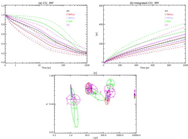
Figure 1 shows the principal results for IRFCO2. Figure 1a

shows IRFCO2 for the reference J07 (black), and for the

four distributions C4MIP(u) (red), C4MIP(c) (blue), LTMIP (green), and J13 (purple) derived from the respective inter-comparison exercises (full lines indicate the median value, dashed lines the 5- and 95-percentile values).

We estimated the J13 IRFCO2 based on the original data,

independent from the estimation presented in Joos et al. (2013). The median of J13 lies very close to the J07 refer-ence. Our 5- and 95-percentile values of 0.47–0.71, 0.33– 0.50, and 0.18–0.30 atH= 20, 100, and 1000 yr, respectively, agree well with the values obtained in Joos et al. (2013). Converting the mean and 2σ values of Joos et al. (2013, Sect. 4.1) into 5- and 95-percentile values gives 0.49–0.71, 0.30–0.52, and 0.18–0.32 atH= 20, 100, and 1000 yr, re-spectively. The experimental setup in J13 is most suited for deriving IRFCO2: the behaviour of the CC-models stays in

the linear regime, and deriving the IRFCO2is reduced to

find-ing the coefficients which best describe the obtained IRFCO2

curve.

The IRFCO2 based on LTMIP is significantly higher than

the standard J07; almost 95 % of its distribution is higher than J07. However, the estimate of the long-term value around year 1000 in LTMIP is again similar to the J07 value. The large differences for earlier times are caused by the very large emission size, i.e. 1000 Gt[C]. This large pulse size intro-duces non-linearities (Joos et al., 2013), as the ocean mixed layer is easily saturated inhibiting a faster take up of atmo-spheric CO2. The fact that the LTMIP experiments were in

the non-linear regime makes the derived IRFCO2less suitable

to be used in metric calculations (where one tries to incorpo-rate the effect of small emission amounts).

The two IRFCO2 based on C

4_{MIP give results slightly}

lower than J07 and J13, and considerably lower than LT-MIP. To guarantee that the CC-models were still in the linear regime, we have used data only up to year 2000 (see Ap-pendix A). For all models in C4MIP(u), the CO2

concentra-tion falls in the range 344–392, 397–465, and 475–570 ppm for the years 2000, 2025, and 2050, respectively, and in 347– 401, 400–483, and 489–604 ppm in C4MIP(c). This limits the length of the time series used to derive the IRFCO2 to

approximately 140 yr, which is considerably shorter than in J13 or LTMIP. In addition, the near-exponential increase in CO2emissions in this experiment might complicate the

esti-mation of IRFCO2. In the case of an exact exponential

emis-sion scenario, quite different IRFCO2 can lead to exactly the

same evolution of the CO2burden (see Eq. 3). This implies

that if more than one mode must be estimated in the IRFCO2,

their weights and timescales can become indeterminate (see Appendix B). However, as the emission scenario here is not exactly exponential, the experiment still contains additional information (Gloor et al., 2010).

One can also see that the results from the coupled exper-iment (c) give larger values for IRFCO2; the increasing

tem-perature in that experiment decreases the net CO2 uptake,

leaving a larger fraction of CO2in the atmosphere. At 100 yr

after the emission, a fraction of 0.31 is still in the atmosphere in C4MIP(c), while it is only 0.28 in C4MIP(u). Joos et al. (2013, Fig. 7) show the impact of the temperature feedback for one model (Bern3D-LPJ) on IRFCO2; for an emission

pulse of 100 Gt[C] they find differences around 15–20 % at 100 yr after the emission.

The spread in J13 is slightly smaller than in LTMIP, but for LTMIP the spread becomes again smaller at the end of the shown horizon range. Both C4MIP IRFCO2 show spreads

comparable with the spread in J13. The 5- and 95-percentile values atH= 100 yr are 0.39–0.69 for LTMIP, 0.21–0.37 for C4MIP(u), 0.24–0.40 for C4MIP(c), and 0.33–0.50 for J13.

Figure 1b shows the time-integrated IRFCO2 for the

(9)

D. J. L. Olivi´e and G. P. Peters: Variation in emission metrics 275

D. J. L. Olivi´e and G. P. Peters: Variation in emission metrics due to variation in impulse response functions 19

(a) CO₂ IRF

0 1 10 100 1000

Time [yr] 0.0

0.2 0.4 0.6 0.8 1.0 1.2

J07

C4_MIP(u)

C4_MIP(c)

LTMIP J13

(b) Integrated CO₂ IRF

0 200 400 600 800 1000

Time [yr] 0

200 400 600

[yr]

J07

C4_MIP(u)

C4_MIP(c)

LTMIP J13

(c)

0.1 1.0 10.0 100.0 1000.0 10000.0

t

i [yr]

0.01 0.10 1.00

ai

Fig. 1. Overview of five different IRFCO2distributions: J07 (black), C 4

MIP(u) (red), C4

MIP(c) (blue), LTMIP (green), and J13 (purple). (a) IRFCO2as in Eq. (1) with median (full line) and 5- and 95-percentile values (dashed lines) indicated. The horizontal axis is linear from 0 to 1 yr, and logarithmic from 1 to 1000 yr. The vertical axis is dimensionless. (b) Integrated IRFCO2. The horizontal axis is linear. (c) Estimates for the parameters in IRFCO2. Every single dot corresponds with one of the four modes, i.e.(τ0,a0)(diamond),(τ1,a1)(triangle),(τ2,a2) (square), or(τ3,a3)(cross). The(τ0,a0)tuples (which would fall off the figure asτ0=∞) are given at the right of the figure. The individual dots represent the best estimates for the individual CC-models, while the ellipses represent the distributions derived from the individual estimates, grouped per inter-comparison exercise. Inside the ellipses falls 90 % of the distribution. The vertical axis is dimensionless.

Fig. 1. Overview of five different IRFCO2 distributions: J07 (black), C

4_{MIP(u) (red), C}4_{MIP(c) (blue), LTMIP (green), and J13 (purple).}

(a) IRFCO2as in Eq. (1) with median (full line) and 5- and 95-percentile values (dashed lines) indicated. The horizontal axis is linear from 0 to

1 yr, and logarithmic from 1 to 1000 yr. The vertical axis is dimensionless. (b) Integrated IRFCO2. The horizontal axis is linear. (c) Estimates

for the parameters in IRFCO2. Every single dot corresponds with one of the four modes, i.e.(τ0, a0)(diamond),(τ1, a1)(triangle),(τ2, a2)

(square), or(τ3, a3)(cross). The(τ0, a0)tuples (which would fall off the figure asτ0= ∞) are given at the right of the figure. The individual

dots represent the best estimates for the individual CC-models, while the ellipses represent the distributions derived from the individual estimates, grouped per intercomparison exercise. Inside the ellipses falls 90 % of the distribution. The vertical axis is dimensionless.

Figure 1c shows best estimates for the parameters of the four modes in IRFCO2 when calibrated to the individual

CC-models. Every single dot corresponds with a tuple(τi, ai)in Eq. (1). The IRFCO2 distributions obtained by combining the

results within the same intercomparison exercise are repre-sented by the ellipses. The area in the ellipses covers 90 % of the distributions. Tilted ellipses indicate that there is a corre-lation between the value ofτiandai. There exist also correla-tions between theaiandτjfrom different modes (i6=j), but they are not represented in this figure. One can see that the J13, C4MIP(u), and C4MIP(c) experiments give parameter values which are not very different from J07. LTMIP gives values which deviate slightly more from J07, e.g. higher val-ues for all the time constants. Also the contributiona1from

the century-like mode is considerably larger, while the con-tribution from the other modes is lower.

The values ofx¯ and6 describing the different derived IRFCO2distributions can be found in Table 5.

4.1.2 Temperature IRF

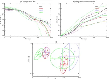
Figure 2 shows the principal results for IRFT. Figure 2a shows IRFT as defined in Eq. (5). We have indicated

the reference distribution from Boucher and Reddy (2008) (black), and the three distributions obtained from the inter-comparison exercise data, i.e. CMIP3 (red), CMIP3* (blue) and CMIP5 (green). One can notice that the CMIP5 IRFT is highest for the first 5 yr (the CMIP5 IRFT starts at 0.17 K W−1m2yr−1, while it starts at 0.076 for BR08 and 0.069 for both CMIP3 and CMIP3*), but the CMIP5 IRFT is lowest in the 100–1000 yr range, where it additionally shows the largest spread (in a logarithmic sense). For the period 100–1000 yr, one can further observe a considerable differ-ence between CMIP3 and CMIP3*, and that CMIP3* is most similar to BR08; for example, at 200 yr we find for BR08, CMIP3, CMIP3*, and CMIP5 the values 6.4, 2.8, 5.5, and 3.0 (×10−4_{K W}−1_m2_yr−1_{). Though, care is needed in}

in-terpreting the results for times of 200 yr and greater as the experimental setups do not cover these time periods well.

(10)

20 D. J. L. Olivi´e and G. P. Peters: Variation in emission metrics due to variation in impulse response functions

(a) Temperature IRF

0 1 10 100 1000

Time [yr] 10-6

10-5

10-4

10-3

10-2

10-1

100

[K W

-1 m 2 yr -1]

BR08

CMIP3 CMIP3* CMIP5

(b) Integrated temperature IRF

0 1 10 100 1000

Time [yr] 0.0

0.2 0.4 0.6 0.8 1.0 1.2

[K W

-1 m 2]

BR08

CMIP3 CMIP3* CMIP5

(c)

1 10 100 1000

t

i [yr]

0.1 1.0

fi

[K W

-1 m 2]

Fig. 2. Overview of four different IRFTdistributions: BR08 (black), CMIP3 (red), CMIP3* (blue), and CMIP5 (green). (a) IRFTas in Eq. (5) with median (full line) and 5- and 95-percentile values (dashed lines) indicated. The horizontal axis is linear from 0 to 1 yr, and logarithmic from 1 to 1000 yr. (b) Integrated IRFTas in Eq. (6). (c) Estimates of the parameters in IRFT. Every single dot corresponds with one of the two modes in a separate AOGCM, i.e., the fast mode(τ1,f1)(diamonds) or the slow mode(τ2,f2)(triangles). The ellipses represent the distributions of the IRFTparameters derived from the individual estimates, grouped per inter-comparison project. Inside the ellipses falls 90 % of the distribution.

Fig. 2. Overview of four different IRFT distributions: BR08 (black), CMIP3 (red), CMIP3* (blue), and CMIP5 (green). (a) IRFT as in Eq. (5) with median (full line) and 5- and 95-percentile values (dashed lines) indicated. The horizontal axis is linear from 0 to 1 yr, and logarithmic from 1 to 1000 yr. (b) Integrated IRFT as in Eq. (6). (c) Estimates of the parameters in IRFT. Every single dot corresponds with one of the two modes in a separate AOGCM, i.e. the fast mode(τ1, f1)(diamonds) or the slow mode(τ2, f2)(triangles). The ellipses

represent the distributions of the IRFT parameters derived from the individual estimates, grouped per intercomparison project. Inside the ellipses falls 90 % of the distribution.

curves fort→ ∞is the climate sensitivity, which is clearly highest for BR08 and CMIP3*. The climate sensitivity shows similar spreads among the IRFT, i.e. 0.4 K for CMIP3, 0.6 K for CMIP5 and 0.7 K for CMIP3* (5–95 % spread). Again, care is needed in interpreting the climate sensitivities as they are often based on short time periods (100–200 yr).

The best estimates for the IRFT parameters when cali-brated to the individual AOGCMs are shown as separate symbols in Fig. 2c. The derived distributions are represented by the ellipses (the area within the ellipses represents 90 % of the distribution). The fast mode shows a response time of the order of 2–10 yr, and the slow mode of the order of 30–500 yr. The CMIP3* approach gives for(τ1, f1)results

similar to CMIP3, but for(τ2, f2)considerably higher

val-ues, reflecting a considerably higher climate sensitivity. The CMIP5 results show relatively small values forτ1, which is

probably related to the type of experiment, i.e. an instanta-neous increase in the radiative forcing (Olivi´e et al., 2012). The CMIP5 results also show lower values for the time con-stant of the slow modeτ2, together with a relatively large

spread in this parameter; this is probably related to the short length of the CMIP5 experiments

The values ofx¯ and6 describing the different derived IRFT distributions can be found in Table 6.

4.2 Impact of variation in IRFs on metrics

Here we present metric values and their variations calculated with the IRF distributions presented above. We use the ex-pressions from Sect. 2 and take into account that the IRFCO2

and IRFT are themselves distributions by performing Monte Carlo simulations. Note that all parameter values such as ra-diative efficiencies, lifetimes of non-CO2species, and

coeffi-cients of the reference IRFCO2 J07 and IRFT BR08 are taken

just as in Forster et al. (2007) and Fuglestvedt et al. (2010). Figure 3 shows the evolution of the GWP, GTP, and iGTP metric as a function of the time horizon for all combina-tions of the four IRFCO2and three IRFT distributions for BC,

CH4, N2O, and SF6. Every combination gives a distribution,

for which only the median is indicated by a black line (how broad the metric distributions are will be shown later). Only 4 lines represent GWP, as there is no dependency on the IRFT. The red lines are the results obtained by combining the ref-erence IRFs J07 and BR08.

Metric values for horizons between 20 and 500 yr fall in the range 1–3000 for BC, 0.1–100 for CH4, 10–400 for N2O,

and 1×104 to 2×104for SF6. The value of the metrics is

(11)

D. J. L. Olivi´e and G. P. Peters: Variation in emission metrics 277

(a) BC

20 50 100 200 500

Time [yr] 1

10 100 1000 10000

GWP

GTP

iGTP

(b) CH₄

20 50 100 200 500

Time [yr] 0.1

1.0 10.0 100.0 1000.0

(c) N

2O

20 50 100 200 500

Time [yr] 10

100 1000

(d) SF

6

20 50 100 200 500

Time [yr] 103

104

105

Fig. 3. Evolution of GWP (full line), GTP (dashed line), and iGTP (dotted line) as a function of the time horizon for (a) BC, (b) CH4, (c) N2O, and (d) SF6, using different combinations of IRFCO2and IRFT. The black curves correspond with all combinations of IRFCO2 distributions (C4MIP(u), C4MIP(c), LTMIP, and J13) and IRFTdistributions (CMIP3, CMIP3*, and CMIP5) – the line shown is the median value of the obtained metric distribution. The red lines are the result of the combination of the reference IRFCO2J07 and IRFTBR08. The vertical axis is dimensionless.

Fig. 3. Evolution of GWP (full line), GTP (dashed line), and iGTP (dotted line) as a function of the time horizon for (a) BC, (b) CH4,

(c) N₂O, and (d) SF₆, using different combinations of IRF_CO₂ and IRF_T. The black curves correspond with all combinations of IRF_CO₂ distributions (C4MIP(u), C4MIP(c), LTMIP, and J13) and IRF_T distributions (CMIP3, CMIP3*, and CMIP5) – the lines shown are the median values of the obtained metric distributions. The red lines are the result of the combination of the reference IRFCO2 J07 and IRFT

BR08. The vertical axis is dimensionless.

variation. For BC and CH4the metric values decay strongly

as a function of the time horizon, for N2O they have the

ten-dency to decay slightly as a function of the time horizon, and for SF6metric values increase as a function of the time

horizon (Tanaka et al., 2009). The GWP and iGTP metric be-have in general very similar, but the behaviour of GTP can be rather different. For a specific species, metric, and time hori-zon, the median values differ in general considerably, up to a factor of two, but the GTPs of BC and CH4show variation

in the median up to a factor of 10 for time horizons of 500 yr or more.

To clarify more the impact of the IRFs on the metrics, we will separately investigate the impact of variation in IRFCO2

and IRFT on metrics. The impact will be decomposed in a

deviation (indicating how much the median value of a metric

differs from the case where the reference IRF is used) and a

spread (indicating how much the 5- and 95-percentile metric

values differ from the median).

4.2.1 Impact of variation in CO2IRF

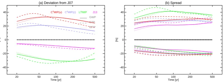
Figure 4 shows the impact of IRFCO2 on GWP, GTP, and

iGTP. We used different IRFCO2 (J07, C

4_{MIP(u), C}4_MIP(c),

LTMIP, and J13), but always the BR08 IRFT to isolate the changes caused by IRFCO2.

Figure 4a shows the difference between the median met-ric value obtained using a specific IRFCO2 and the value

ob-tained using the reference J07. As variation in IRFCO2 only

affects the denominator in the expression for GWP, GTP, or iGTP, and as this denominator is equal for all species, the impact from variation in IRFCO2 is identical for all the four

species we study here. The LTMIP and J13 IRFCO2 lead to

lower values than J07 (around−25 % for LTMIP and−5 % to−15 % for J13). These lower values reflect the fact that the LTMIP and J13 IRFCO2 are higher than the J07 IRFCO2

(see Fig. 1a). The median metric values from C4MIP(u) and C4MIP(c) are significantly higher than the J07 values (10– 40 %). This is caused by the fact that both C4MIP IRFCO2

are lower than the J07 IRFCO2.

Figure 4a also shows that the impact of variation in IRFCO2

is similar for the three metrics (GWP, GTP, and iGTP). The closest agreement can be seen between GWP and iGTP (Pe-ters et al., 2011). Also the variation of the metrics as a func-tion of the time horizon or choice of IRFCO2 is very similar

for the three metrics, although the maximum deviation is sit-uated at shorter time horizons for GTP than for GWP and iGTP.

The C4MIP(u) IRFCO2 gives 10 % higher metric values

(12)

278 D. J. L. Olivi´e and G. P. Peters: Variation in emission metrics

(a) Deviation from J07

20 50 100 200 500

Time [yr] -40

-20 0 20 40

[%]

C4 MIP(u) C4

MIP(c) LTMIP J13

GWP

GTP

iGTP

(b) Spread

20 50 100 200 500

Time [yr] -40

-20 0 20 40

[%]

Fig. 4. Impact of variation in IRFCO2on GWP (full line), GTP (dashed line), and iGTP (dotted line), using the C4MIP(u) (red), C4MIP(c) (blue), LTMIP (green), and J13 (purple) IRFCO2. (a) Difference between the median of the obtained metric distribution and the value obtained using the reference J07 IRFCO2. (b) Spread of the obtained metric distribution, indicating the difference between the 5-percentile and the median value (lower lines), and between the 95-percentile and median value (upper lines). These impacts are equal for all species (BC, CH4, N2O, and SF6).

(a) Deviation from BR08

20 50 100 200 500

Time [yr] -100

-50 0 50 100

[%]

BC CH

4 N2O SF6 CMIP3

CMIP3*

CMIP5

(b) Spread

20 50 100 200 500

Time [yr] -100

-50 0 50 100

[%]

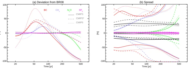
Fig. 5. Impact of variation in IRFTon GTP for BC (red), CH4(blue), N2O (green), and SF6(purple), using the CMIP3 (full line), CMIP3* (dashed line), and CMIP5 (dotted line) IRFT. (a) Difference between the median of the obtained metric distribution and the value obtained using the reference BR08 IRFT. (b) Spread of the obtained metric distribution, indicating the difference between the 5-percentile and the median value (lower lines), and between the 95-percentile and median value (upper lines). The black lines show the spread induced by IRFCO2on GTP from C

4

MIP(u) (full line), C4

MIP(c) (dotted line), LTMIP (dashed line), and J13 (dot-dashed line) – these lines are identical to the dashed lines in Fig. 4b.

Fig. 4. Impact of variation in IRF_CO₂ on GWP (full line), GTP (dashed line), and iGTP (dotted line), using the C4MIP(u) (red), C4MIP(c) (blue), LTMIP (green), and J13 (purple) IRFCO2. (a) Difference between the median of the obtained metric distribution and the value obtained

using the reference J07 IRF_CO₂. (b) Spread of the obtained metric distribution, indicating the difference between the 5-percentile value and the median value (lower lines), and between the 95-percentile value and median value (upper lines). These impacts are equal for all species (BC, CH4, N2O, and SF6).

(2013, Sect. 4.4.3 and Fig. 7), who investigated the impact of the temperature feedback with one CC-model, found an impact of 13 % on the integrated IRFCO2 at time horizons

of 100 and 500 yr for a pulse emission size of 100 Gt[C]. Slightly smaller impacts are found for time horizons shorter than 100 yr or longer than 500 yr.

Figure 4b shows the spread of the metric values, indicat-ing how much the 5- and 95-percentile values differ from the median value. Again, these spreads are identical for all species, and one can see that these spreads do not vary much among the different metrics. The differences fall in the range of−20 to+40 %, and are not very sensitive to the value of the time horizon. The LTMIP IRFCO2induces a slightly more

asymmetric spread than the other IRFCO2, which is most

pro-nounced for short time horizons. This is a consequence of the asymmetric LTMIP IRFCO2, as can be seen in Fig. 1a.

The variation in the GWP estimates presented here is solely caused by variation in its denominator AGWPCO2,

implying that the variation we estimated for GWP, actually also gives the variation in AGWPCO2. Joos et al. (2013,

Ta-ble 4) indicate spreads for AGWPCO2. Converting their 2σ

values for AGWPCO2 into 5- and 95-percentile values gives

forH= 20, 50, 100, and 500 yr the ranges±10,±15,±18, and±21 %, respectively. These values agree well with the impacts we found of−9 to+16 %,−13 to +21 %,−14 to +22 %, and−18 to +25 % (see purple full line in Fig. 4b, or later see Fig. 6). Reisinger et al. (2010) have also estimated uncertainties on the AGWPCO2. Their 5–95 % confidence

in-terval values for AGWPCO2 (based on their AOGCM/C

4_MIP

model evaluation) give−17 to+19 %,−23 to+26 %, and

−25 to+22 % forH= 20, 100, and 500 yr, respectively. Al-though they included also the impact of uncertainty in radia-tive efficiencies, their variations are comparable to our val-ues. In Reisinger et al. (2011) the 5- to 95-percentile range in GWPCH4 and GWPN2Ois estimated to be−15 to+20 % for H= 20 yr and−20 to+30 % forH= 100 and 500 yr, which is in fair agreement with our estimates.

4.2.2 Impact of variation in temperature IRF

The GTP and iGTP metric values also depend on IRFT. We investigate this by using the reference J07 IRFCO2, but

differ-ent IRFT (BR08, CMIP3, CMIP3*, and CMIP5). This vari-ation influences both the numerator and denominator in the expression for GTP and iGTP (see Eqs. 9 to 12). We mainly concentrate on GTP, as iGTP is much less influenced.

Figure 5 shows the impact of variation in IRFT on GTP. Figure 5a shows the deviation of the median value from the value obtained using the reference IRFT. In contrast to the impact of IRFCO2, the impact now differs among species.

N2O and SF6 show very small variations due to variation

in IRFT, while BC shows a deviation of the median from the reference value in the range of−90 to+85 %, and for CH4 in the range of−90 to +45 %. We see, for example,

that for BC and CH4using the CMIP3, CMIP3*, or CMIP5

IRFT gives lower metric values with respect to BR08 for the smallest time horizon (H= 20 yr), but higher values for

H= 50 yr, and this is most pronounced for the CMIP5 IRFT. This behaviour can be explained by noting that GTPBCis the

ratio of AGTPBCand AGTPCO2. As BC has a very short

life-time, the time dependence of AGTPBCis very similar to the

IRFT curve in Fig. 2a. On the other hand, because CO2has

characteristics of a longer lifetime, the time dependence of AGTPCO2 will be more similar to the integrated IRFT curve

(13)

D. J. L. Olivi´e and G. P. Peters: Variation in emission metrics 279

(a) Deviation from J07

20 50 100 200 500

Time [yr] -40

-20 0 20 40

[%]

C4_MIP(u) _C4_MIP(c) _LTMIP _J13

GWP

GTP

iGTP

(b) Spread

20 50 100 200 500

Time [yr] -40

-20 0 20 40

[%]

Fig. 4. Impact of variation in IRFCO2on GWP (full line), GTP (dashed line), and iGTP (dotted line), using the C4

MIP(u) (red), C4 MIP(c) (blue), LTMIP (green), and J13 (purple) IRFCO2. (a) Difference between the median of the obtained metric distribution and the value obtained using the reference J07 IRFCO2. (b) Spread of the obtained metric distribution, indicating the difference between the 5-percentile and the median value (lower lines), and between the 95-percentile and median value (upper lines). These impacts are equal for all species (BC, CH4, N2O, and SF6).

(a) Deviation from BR08

20 50 100 200 500

Time [yr] -100

-50 0 50 100

[%]

BC CH

4 N2O SF6 CMIP3

CMIP3*

CMIP5

(b) Spread

20 50 100 200 500

Time [yr] -100

-50 0 50 100

[%]

Fig. 5. Impact of variation in IRFTon GTP for BC (red), CH4(blue), N2O (green), and SF6(purple), using the CMIP3 (full line), CMIP3* (dashed line), and CMIP5 (dotted line) IRFT. (a) Difference between the median of the obtained metric distribution and the value obtained using the reference BR08 IRFT. (b) Spread of the obtained metric distribution, indicating the difference between the 5-percentile and the median value (lower lines), and between the 95-percentile and median value (upper lines). The black lines show the spread induced by IRFCO2on GTP from C4

MIP(u) (full line), C4

MIP(c) (dotted line), LTMIP (dashed line), and J13 (dot-dashed line) – these lines are identical to the dashed lines in Fig. 4b.

Fig. 5. Impact of variation in IRFT on GTP for BC (red), CH4(blue), N2O (green), and SF6(purple), using the CMIP3 (full line), CMIP3*

(dashed line), and CMIP5 (dotted line) IRFT. (a) Difference between the median of the obtained metric distribution and the value obtained using the reference BR08 IRFT. (b) Spread of the obtained metric distribution, indicating the difference between the 5-percentile value and the median value (lower lines), and between the 95-percentile value and median value (upper lines). The black lines show the spread induced by IRFCO2on GTP from C

4_{MIP(u) (full line), C}4_{MIP(c) (dotted line), LTMIP (dashed line), and J13 (dot-dashed line); these lines}

are identical to the dashed lines in Fig. 4b.

to CO2. One can note that for time horizons of 200 yr and

longer, the curves for BC (red) and CH4(blue) have the

ten-dency to coincide. One can also see that for BC and CH4and

for time horizons between 200 and 500 yr, CMIP3* (dashed line) gives a smaller deviation than CMIP3 or CMIP5.

The generally small deviations for N2O and SF6 from

BR08 for the time horizons considered are caused by the fact that AGTPN2Oand AGTPSF6, as a function of time, behave

similarly to the integrated IRFT (as long as the horizon is not much longer than the lifetime of the species). CO2has a

similar dependence on IRFT (see above). As a consequence, the variations in the numerator and denominator of the GTP expression due to variations in the IRFT will be similar and largely cancel out in the expression for GTPN2Oand GTPSF6.

As this condition is not fulfilled with N2O for time horizons

longer than 200 yr, GTN2Ostarts to deviate from there on.

Figure 5b shows the spread in GTP values due to varia-tion in IRFT. The amount of spread is strongly dependant on the species and the time horizon. For time horizons up toH= 100 yr, BC shows variations in the range of−60 to

+80 %, and this spread increases drastically for longer time horizons. For CH4, the spread is smaller than for BC when

looking at time horizons of 20 and 50 yr, but rather similar for longer ones. For N2O, very small ranges are found up to

time horizons of 100 yr, but increasing after that. For SF6we

find small spreads for all time horizons.

For comparing the impact of variation in IRFCO2 and

IRFT, Fig. 5b also shows the impact of IRFCO2 in black

(these lines correspond with the dashed lines from Fig. 4b). One can see that the spread in GTP for BC is dominated by IRFT, and for CH4 by IRFCO2 at short time horizons

(H= 20 yr) and by IRFT at longer time horizons. For N2O

and SF6 it is dominated by variation in IRFCO2, except for

N2O at time horizons longer than 200 yr.

Reisinger et al. (2010) present also values for the variation in GTPCH4 forH= 20, 100, and 500 yr, i.e.−26 to+30 %, −48 to+77 %, and−101 to+172 %, respectively (we de-rived the value forH= 100 yr from their Table 2). This vari-ation clearly increases as a function of the time horizon, in accordance to our findings.

For iGTP one finds much lower impacts of the variation from IRFT (not shown), since iGTP is an integrated version of GTP. The deviations are of the order of 5 %, except for BC atH= 20 yr using the CMIP5 IRFT where the deviation reaches−15 %. Spreads are in general smaller than±10 %. The much smaller variation in iGTP with respect to GTP, e.g. for BC, can be explained by the fact that the numerator in iGTP is now the integral of the curve shown in Fig. 2a. As the CMIP5 curve up to 20 yr lies partially above and partially below the BR08 curve, the integrals are not that different for

H= 20 yr. For longer time horizons this difference is even further reduced. Accordingly, also the spread is strongly re-duced.

Finally, for two selected IRFs, i.e. the J13 IRFCO2 and the

CMIP5 IRFT, Fig. 6 shows the impact of IRF variation on GWP, GTP, and iGTP for BC, CH4, N2O, and SF6at specific

time horizons of 20, 50, 100, 200, and 500 yr. It shows the impact from variation in IRFCO2, from variation in IRFT, and

from variation in both IRFCO2 and IRFT.

4.3 Synthesis of results

The aim of this study was twofold. The first aim was to de-rive IRFCO2 and IRFT distributions based on the behaviour

of different CC-models and AOGCMs. The second aim was to analyse how variation in these IRFs influences common emission metrics.

(14)

GWP BC H=20 H=50 H=100 H=200 H=500 1500

1.00 -9% 16%

715

1.00 -13% 21%

413

1.00 -14% 22%

239

1.01 -15% 23%

120

1.01 -18% 25%

0 1000 2000 3000

CH 4 H=20 H=50 H=100 H=200 H=500 67.9

1.00 -9% 16%

39.2

1.00 -13% 21%

23.0

1.00 -14% 22%

13.3

1.01 -15% 23%

6.7

1.01 -18% 25%

0 50 100 150

N 2O H=20 H=50 H=100 H=200 H=500 273

1.00 -9% 16%

286

1.00 -13% 21%

272

1.00 -14% 22%

223

1.01 -15% 23%

134

1.01 -18% 25%

0 200 400 600

SF 6 H=20 H=50 H=100 H=200 H=500 15300

1.00 -9% 16%

18100

1.00 -13% 21%

20700

1.00 -14% 22%

23600

1.01 -15% 23%

28300

1.01 -18% 25%

0 20000 40000

GTP BC H=20 H=50 H=100 H=200 H=500 210 1.00 1.00 1.03 -14% 25% -59% 86% -60% 89% 154 1.00 0.84 0.84 -16% 25% -62% 59% -62% 67% 85.1 1.00 0.82 0.82 -16% 25% -88% 64% -89% 74% 27.2 1.01 0.96 0.95 -19% 29% -100% 133% -100% 149% 0.9 1.01 0.99 0.98 -23% 33% -100% 2300% -100% 2300%

0 500 1000

CH 4 H=20 H=50 H=100 H=200 H=500 42.8 1.00 1.01 1.02 -14% 25% -8% 10% -16% 26% 12.7 1.00 0.93 0.93 -16% 25% -36% 37% -38% 48% 5.6 1.00 0.83 0.83 -16% 25% -76% 57% -76% 68% 1.8 1.01 0.94 0.94 -19% 29% -99% 120% -99% 131% 0.1 1.01 0.96 0.96 -23% 33% -100% 2200% -100% 2100%

0 50 100

N 2O H=20 H=50 H=100 H=200 H=500 291 1.00 1.00 1.00 -14% 25% -1% 1% -13% 24% 290 1.00 1.00 1.00 -16% 25% 0% 0% -16% 25% 236 1.00 0.99 0.99 -16% 25% -3% 3% -17% 24% 138 1.01 0.97 0.98 -19% 29% -15% 12% -23% 31% 17.8 1.01 1.00 1.02 -23% 33% -38% 145% -45% 150%

0 200 400 600

SF 6 H=20 H=50 H=100 H=200 H=500 17200 1.00 1.00 1.00 -14% 25% -2% 2% -13% 25% 21300 1.00 1.00 1.00 -16% 25% -3% 2% -17% 25% 24300 1.00 1.01 1.01 -16% 25% -2% 3% -17% 24% 28100 1.01 1.00 1.02 -19% 29% -3% 3% -19% 29% 34900 1.01 1.00 1.00 -23% 33% -4% 1% -23% 33%

0 25000 50000

iGTP BC H=20 H=50 H=100 H=200 H=500 1780 1.00 1.01 1.02 -9% 15% -5% 7% -10% 15% 822 1.00 0.99 1.00 -13% 21% -5% 6% -14% 21% 476 1.00 0.98 0.98 -14% 21% -5% 6% -15% 22% 270 1.01 0.99 0.99 -15% 22% -6% 6% -16% 23% 127 1.01 1.00 1.02 -18% 25% -4% 8% -19% 25%

0 2000 4000

CH 4 H=20 H=50 H=100 H=200 H=500 72.3 1.00 1.00 1.00 -9% 15% -2% 2% -9% 14% 42.9 1.00 1.00 1.00 -13% 21% -3% 4% -13% 21% 25.9 1.00 0.99 0.99 -14% 21% -4% 5% -15% 22% 14.9 1.01 0.99 0.99 -15% 22% -6% 6% -16% 22% 7.1 1.01 1.00 1.02 -18% 25% -4% 8% -19% 26%

0 50 100 150

N 2O H=20 H=50 H=100 H=200 H=500 269 1.00 1.00 1.00 -9% 15% 0% 0% -9% 14% 285 1.00 1.00 1.00 -13% 21% 0% 0% -13% 20% 275 1.00 1.00 1.00 -14% 21% 0% 0% -14% 21% 231 1.01 1.00 1.00 -15% 22% -1% 1% -15% 21% 140 1.01 1.00 1.01 -18% 25% -3% 4% -18% 25%

0 200 400 600

SF 6 H=20 H=50 H=100 H=200 H=500 14900 1.00 1.00 1.00 -9% 15% -1% 1% -9% 14% 17700 1.00 1.00 1.00 -13% 21% -1% 1% -13% 20% 20300 1.00 1.00 1.00 -14% 21% -1% 1% -14% 21% 23200 1.01 1.00 1.01 -15% 22% -1% 1% -15% 21% 27900 1.01 1.00 1.01 -18% 25% -1% 1% -18% 25%

0 20000 40000

Fig. 6. Impact of variation in J13 IRFCO2and CMIP5 IRFT on GWP, GTP, and iGTP values for BC, CH4, N2O, and SF6for time horizons

of 20, 50, 100, 200, and 500 yr. The red bars give the impact of variation in IRFCO2, the blue bars the impact of variation in IRFT, and the

green bars the impact of variation in both IRFCO2and IRFT. For every time horizon, the little black line (top) represents the reference value

of the metric using the parameters as given in Tables 3 and 4 in the IRFs – the value itself is indicated right of the little line. The left bars give the 5-, 25-, 50-, 75-, and 95-percentile values of the metric (the 50-percentile value is indicated by a black line). The number right of the bar indicates how much the median value deviates from the reference value in relative terms. The right bars indicate the spread with respect to the median value, where again the 5-, 25-, 75-, and 95-percentile values are represented. The numbers (in %) left and right of the bars indicate how much the 5- and 95-percentile value deviate from the median value. The horizontal axis which gives the value of the metric is dimensionless.

Fig. 6. Impact of variation in J13 IRFCO2 and CMIP5 IRFT on GWP, GTP, and iGTP values for BC, CH4, N2O, and SF6for time horizons

of 20, 50, 100, 200, and 500 yr. The red bars give the impact of variation in IRFCO2, the blue bars the impact of variation in IRFT, and the

green bars the impact of variation in both IRF_CO₂ and IRF_T. For every time horizon, the little black line (top) represents the reference value of the metric using the parameters as given in Tables 3 and 4 in the IRFs – the value itself is indicated to the right of the little line. The left bars give the 5-, 25-, 50-, 75-, and 95-percentile values of the metric (the 50-percentile value is indicated by a black line). The number right of the bar indicates how much the median value deviates from the reference value in relative terms. The right bars indicate the spread with respect to the median value, where again the 5-, 25-, 75-, and 95-percentile values are represented. The numbers (in %) left and right of the bars indicate how much the 5- and 95-percentile values deviate from the median value. The horizontal axis which gives the value of the metric is dimensionless.

IRFCO2 distributions, and CMIP3 and CMIP5 for

estimat-ing IRFT distributions. As reference for comparison we have taken the IRFCO2 from Forster et al. (2007) (in the text noted

as J07) and the IRFT from Boucher and Reddy (2008) (in the text noted as BR08).

The J13 IRFCO2 is similar to the reference J07 IRFCO2,

but the behaviour of the other three derived IRFCO2 is rather

different from the reference. The similarity between J07 and J13 reflects similar experimental setups, and differences in experimental setup explain the differences between J07, LT-MIP, and C4MIP. The LTMIP IRFCO2 has a tendency to

remain considerably higher than J07, giving similar values to J07 only after 1000 yr. These differences relate to non-linearities caused by the large pulse and different background

in LTMIP. The C4MIP IRFCO2 is considerably lower than

the J07 IRFCO2. The relatively short time series and

grad-ually changing emission scenario in C4MIP (as opposed to pulse emissions in J07, J13, and LTMIP) lead to a lower con-fidence in the value of IRFCO2 for short times (below 3–5 yr)

and long times (above 500 yr).

Similar spreads in the IRFCO2 are found for J13,

C4_{MIP(u), and C}4_{MIP(c). For LTMIP, the width increases}

slightly stronger as a function of time, and the width of the distribution decreases again for long timescales (100– 1000 yr). In general, the order of magnitude of the width of the distributions is similar for all four IRFCO2.

(15)