Polarization data from SCIAMACHY limb backscatter observations compared to vector radiative transfer model simulations

(1)

Atmos. Meas. Tech., 6, 1503–1520, 2013 www.atmos-meas-tech.net/6/1503/2013/ doi:10.5194/amt-6-1503-2013

EGU Journal Logos (RGB)

Advances in

Geosciences

Open Access

Natural Hazards

and Earth System

Sciences

Open Access

Annales

Geophysicae

Open Access

Nonlinear Processes

in Geophysics

Open Access

Atmospheric

Chemistry

and Physics

Open Access

Atmospheric

Chemistry

and Physics

Open Access

Discussions

Atmospheric

Measurement

Techniques

Open Access

Atmospheric

Measurement

Techniques

Open Access

Discussions

Biogeosciences

Open Access Open Access

Biogeosciences

Discussions

Climate

of the Past

Climate

of the Past

Discussions

Earth System

Dynamics

Earth System

Dynamics

Discussions

Geoscientific

Instrumentation

Methods and

Data Systems

Open Access

Geoscientific

Instrumentation

Methods and

Data Systems

Open Access

Discussions

Geoscientific

Model Development

Geoscientific

Model Development

Discussions

Hydrology and

Earth System

Sciences

Open Access

Hydrology and

Earth System

Sciences

Open Access

Discussions

Ocean Science

Discussions

Solid Earth

Discussions

The Cryosphere

Discussions

Natural Hazards

and Earth System

Sciences

Open Access

Discussions

Polarization data from SCIAMACHY limb backscatter observations

compared to vector radiative transfer model simulations

P. Liebing, K. Bramstedt, S. No¨el, V. Rozanov, H. Bovensmann, and J. P. Burrows

University of Bremen, Institute of Environmental Physics, P.O. Box 33 04 40, 28334 Bremen, Germany

Correspondence to: P. Liebing ([email protected])

Received: 9 February 2012 – Published in Atmos. Meas. Tech. Discuss.: 15 March 2012 Revised: 16 April 2013 – Accepted: 29 April 2013 – Published: 5 June 2013

Abstract. SCIAMACHY is a passive imaging

spectrome-ter onboard ENVISAT designed to obtain trace gas abun-dances from measured radiances and irradiances in the UV to SWIR range in nadir-, limb- and occultation-viewing modes. Its grating spectrometer introduces a substantial sensitivity to the polarization of the incoming light with nonnegligible effects on the radiometric calibration. To be able to correct for the polarization sensitivity, SCIAMACHY utilizes broad-band Polarization Measurement Devices (PMDs). While for the nadir-viewing mode the measured atmospheric polariza-tion has been validated against POLDER data (Tilstra and Stammes, 2007, 2010), a similar validation study regarding the limb-viewing mode has not yet been performed. This pa-per aims at an assessment of the quality of the SCIAMACHY limb polarization data. Since limb polarization measure-ments by other air/spaceborne instrumeasure-ments in the spectral range of SCIAMACHY are not available, a comparison with radiative transfer simulations by SCIATRAN V3.1 (Rozanov et al., 2013) using a wide range of atmospheric parameters is performed. SCIATRAN is a vector radiative transfer model (VRTM) capable of performing calculations of the multiply scattered radiance in a spherically symmetric atmosphere.

The study shows that the limb polarization data exhibit a large time-dependent bias that decreases with wavelength. Possible reasons for this bias are a still unknown combination of insufficient accuracy or inconsistencies of the on-ground calibration data, scan mirror degradation and stress induced changes of the polarization response of components inside the optical bench of the instrument. It is shown that it should in principle be feasible to recalibrate the effective polariza-tion sensitivity of the instrument using the in-flight data and VRTM simulations.

1 Introduction

SCIAMACHY (SCanning Imaging Absorption spectroM-eter for Atmospheric CHartographY) is in a polar sun-synchronous orbit onboard ESA’s ENVISAT platform. It ob-tains spectra of the solar radiance as it is reflected, scattered or transmitted by the Earth in limb-, nadir- as well as solar and lunar occultation-viewing modes by means of a grating spectrometer with moderate spectral resolution between 0.2 and 1.5 nm (Bovensmann et al., 1999). Its spectral range cov-ers the region between 240 and 1700 nm as well as two bands around 2 and 2.4 µm. In a typical orbit, limb and nadir scans are alternated such that their footprints overlap. Limb scans are typically performed in 30 steps of about 3.3 km from just below the horizon to about 93 km, with a total horizontal scan size of about 960 km. In each horizontal scan 4 mea-surements are taken, resulting in an effective field of view (FoV) of about 260 km across track and 2.6 km vertically at the tangent point. The limb scans performed on the day side of each orbit cover a range of solar zenith angles between 20 and 90◦and relative azimuth angles between 20 and 160◦. An overview of the instrument design and its features is given in Gottwald and Bovensmann (2011).

(2)

instrument throughput can be up to 40 %·P different for light with a degree of polarizationP compared to unpolar-ized light. The polarization of the scattered sunlight follows a generic pattern along the (sun-synchronous) orbit given by the specific scattering geometry of each limb scan. Its vari-ability increases with wavelength due to the increasing influ-ence of scattering on aerosols, cloud droplets and the surface compared to pure Rayleigh scattering on molecules. Radio-metric errors arising from uncorrected polarization sensitiv-ity could be as high as 20 % and lead to systematic errors depending on latitude and season, directly in the reflectance measurements but possibly also indirectly in derived prod-ucts such as trace gas or aerosol concentrations.

The instrument’s polarization sensitivity was measured in a dedicated on-ground calibration campaign. To be able to correct the measured signals for the polarization-dependent throughput, the polarization is measured by the so-called Polarization Measurement Devices (PMDs) in 5 differ-ent wavelength bands whose average wavelength roughly matches with the central wavelength in SCIAMACHY chan-nels 2 to 6. In this way it is in principle possible to de-termine a smoothed polarization spectrum between 300 and 1700 nm1. It is not possible to obtain measurements of spec-tral features in the polarization arising from strong trace gas absorption where the photon light path is significantly al-tered, or from Raman scattering around Fraunhofer lines. The PMDs are sampling detectors with high sensitivity to light polarized parallel to the instrument’s entrance slit. An addi-tional PMD is particularly sensitive to 45◦polarized light in the same spectral range as PMD 4 around 850 nm.

The polarization measurements benefit not only the accu-rate radiometric calibration of SCIAMACHY radiance spec-tra, they could also provide valuable information on micro-physical parameters of aerosols and clouds (Lebsock et al., 2007). Radiance data alone, in particular if only a single viewing direction per scanned air volume is available, can usually not resolve the ambiguities between effects of the surface albedo, the aerosol concentration and its microscopic properties (Kokhanovsky et al., 2007). The addition of po-larization information could in principle provide constraints on different aerosol models. This is in general true for both nadir- and limb-viewing modes. Global sets of dedicated multispectral and multiview nadir polarization measurements are available from the POLDER instruments (Deschamps et al., 1994) onboard ADEOS, ADEOS-II and PARASOL (Br´eon et al., 2002). GOME (Burrows et al., 1999) and GOME-2 (Munro et al., 2006) measure the nadir polariza-tion in a similar manner to SCIAMACHY (Krijger et al., 2004; Callies et al., 2002). CALIOP on CALIPSO

pro-1_{A sixth PMD is installed for the 2}_.₀_{< λ <}₂_._{4 µm range;}

how-ever, the corresponding SCIAMACHY pixel detectors cover only one third of its wavelength range. Because of this and due to hard-ware problems in both the PMD and the pixels detectors, polariza-tion values obtained from PMD 6 are therefore highly unreliable.

vides lidar depolarization measurements at 532 nm with good height resolution but small spatial coverage (Winker et al., 2009). Aside from SCIAMACHY, limb polarization mea-surements are only available from a number of aircraft mis-sions (McLinden et al., 1999). Indirect measurements in the UV region have been performed as part of O3retrievals from

OSIRIS spectra (McLinden et al., 2004). SCIAMACHY, however, has the unique potential to provide the only con-tiguous and global limb polarization profile data available, now spanning almost 10 years.

In light of this it is vital to validate the SCIAMACHY limb polarization data. Due to the lack of both polarized internal calibration sources and independent measurements, the validation has to be performed against a radiative trans-fer model capable of simulating the Stokes vector of the limb-scattered intensity in a spherical atmosphere. This pa-per presents a comparison of limb polarization data from SCIAMACHY obtained between 2004 and 2010 with SCI-ATRAN (version 3.1) simulations for a wide range of atmo-spheric scenarios. An investigation of possible instrumental and theoretical error sources has been performed. The possi-bility of using model simulations for in-flight calibration of the polarization sensitivity will also be discussed, and first results will be shown.

In Sect. 2, the measurement and calibration methods rele-vant for the determination of the polarization are introduced. The selection of the data set used for this study is moti-vated. Section 3 gives a brief overview of SCIATRAN and the setup for the simulations. A comparison of the simula-tions and the data on a statistical basis is presented in Sect. 4. An investigation of possible error sources and a discussion of options for the in-flight calibration and monitoring are discussed together with first results in Sect. 5.

2 Measurement method and data selection

2.1 General calibration and measurement concept

The algorithm to determine the polarization makes use of the Mueller matrix formalism. Sunlight reflected and scattered into the instrument FoV can be described by the components of a Stokes vector:

I=



  

I Q U V



  

, (1)

whereI is the total intensity in photons s−1_sr−1_nm−1_cm−2

and

Q=Ik−I⊥, U=I45◦−I₋₄₅◦. (2)

(3)

The end-to-end Mueller matrix M describes the instrument response to each of the Stokes vector components:

Sdet=[M·I]0=I M11

1+M12

M11

Q

I +

M13

M11

U

I

. (3)

The detector signalSdet=Sraw−Soffset (i.e., the raw ADC

signal corrected for all additive contributions such as pedestal and dark current) is the first component of the resulting Stokes vector; therefore, in Eq. (3) only the first row of the Mueller matrix is relevant. The circular component of the atmospheric polarization is negligibly small (Hansen and Travis, 1974) such that the detected signal can be described in terms of the total intensity, the absolute radiance sensitiv-ityM11, the relative polarization sensitivities

µi=

M1i

M11

, i=2,3 (4)

and the degrees of polarization of the second and third Stokes components:q=Q

I andu=

U

I.

The wavelength-dependent Mueller matrix includes the re-sponse of both the Optical Bench Module (OBM) and the scanner module. As in each SCIAMACHY measurement mode a different setup of the scanner module is used, the Mueller matrix depends on the measurement mode and the involved scan angles. For limb measurements, the Mueller matrix includes the effects of the elevation scan module (ESM) as well as the azimuth scan module (ASM) mir-rors. The OBM comprises all components behind the scanner module. The Mueller matrix elements (MMEs) are derived from on-ground measurements of the polarization sensitivity (the so-called “Greek” calibration key data).

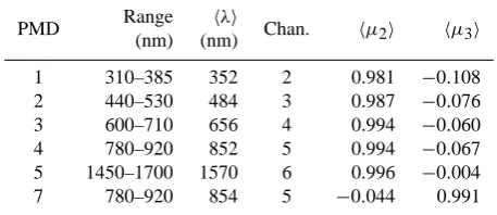
Every polarization measurement requires the determina-tion of at least two independent observables of the same light beam. The measurement approach taken for SCIAMACHY is to split the incoming light into two beams with known fraction and measure the signal in two detectors with differ-ent, known polarization sensitivity. The predisperser prism behind the entrance slit to the telescope generates one fully polarized beam directed towards the PMDs and one beam that is further processed by the spectrometer and recorded by the science pixel detectors. The PMDs sample the signal at a frequency of 40 Hz. The PMD signals have to be synchro-nized to the integrated signal of the detector pixels and inte-grated over the exposure time of the corresponding science detectors. In total, seven PMDs are installed, where PMDs 1–6 are mostly sensitive toQand PMD 7 is sensitive toU. Table 1 lists the PMDs with their spectral range and average wavelengths for typical limb spectra. PMD 6, which is sen-sitive in the 2.0< λ <2.4 µm range, will not be discussed here because its polarization values are not meaningful due to lack of corresponding science detector coverage. A more detailed description of the calibration concept can be found in Gottwald and Bovensmann (2011).

Table 1. SCIAMACHY PMDs, their spectral range, average

wave-length, corresponding SCIAMACHY science channel and average polarization sensitivities for limb measurements.

PMD Range_(nm) _(nm)hλi Chan. hµ2i hµ3i

1 310–385 352 2 0.981 −0.108 2 440–530 484 3 0.987 −0.076 3 600–710 656 4 0.994 −0.060 4 780–920 852 5 0.994 −0.067 5 1450–1700 1570 6 0.996 −0.004 7 780–920 854 5 −0.044 0.991

2.2 Determination of polarization values

The operational polarization algorithm makes use of the fact that the intensities corresponding to the integrated signals of the science pixels and the PMDs have to be the same. The signals of thei-th pixel of the science channel and thei-th (virtual) pixel of the PMD according to Eq. (3) are:

S_iD(P)=I M₁₁D(_,iP)1+µ₂D_,i(P)q+µ₃D_,i(P)u. (5)

The integrated signals of the science channel over the spec-tral range of the PMD and PMD signal can then be related to each other by

IB·SP=X i

S_iDM₁PD_,i 1

+µP₂_,iq+µP₃_,iu

1+µD₂_,iq+µD₃_,iu , with (6)

M₁PD_,i =M

P 11,i

M₁₁D_,i . (7)

The superscripts P and D refer to PMD and pixel detectors, respectively, and the sum is over all pixels from the start to the end of the PMD spectral range. The sum on the right-hand side of Eq. (6) is called virtual sum, and Eq. (6) is called virtual sum equation. The scale factor IB is the so-called in-band signal and should account for initial calibration errors in the radiance response ratioM₁PD, for gaps (due to bad pix-els) or cutoffs in the pixel detector range and for degrada-tion effects. It is determined from solar reference measure-ments, which are performed daily, and ensures that for un-polarized light (q=0, u=0) the scaled PMD signal is equal to the virtual sum. However, since the spectral shape of the solar irradiance in the reference measurements is very differ-ent from that of the limb and nadir Earth shine spectra, and since each measurement mode uses a different scanner con-figuration, the in-band signal may actually cause a constant polarization bias.

(4)

over the corresponding wavelength range. As the two mea-surements allow only the determination of one polarization component, the assumption

u/q=const.=uSS/qSS (8)

is made, withuSS/qSSbeing the ratio ofuandq for single

Rayleigh scattering. This assumption was justified by model studies representative for nadir conditions (Schutgens et al., 2004). SCIATRAN simulations performed for this study showed that the assumption is well justified above 500 nm in the nadir mode. In the UV between 300 and 400 nm, the ra-tio is not constant, although in most cases the resulting errors on u are below 0.1. For the limb mode, SCIATRAN sim-ulations in general indicate a higher variability of theu/q

ratio with consequent errors onuof up to 0.2 even at visi-ble wavelengths. However, as discussed below in Sect. 3.1, intrinsic model errors in SCIATRAN currently inhibit quan-titative conclusions on this issue. In the case of very small

|qSS|,uis assumed to bec·uSSwithca factor, depending

on mode and wavelength, determined from model studies (Slijkhuis, 2008). The on-ground key data suggest that the PMD sensitivity tougiven byµP₃ is relatively small, except for PMD 1 (see Table 1). Errors related to the assumption onuare therefore usually also small. However, this is only true as long as|µP₂qSS| |µP₃uSS|. If both terms are roughly

equal and nearly cancel each other, a value of the virtual sum around 1 will be misinterpreted as a small value ofqandu. This may result in large errors of the polarization values as well as the polarization correction term. This issue will be further discussed in Sect. 5.1.

The Stokes vector and Mueller matrix need to be defined in a common reference frame. The current operational pro-cessor (version 7.03) uses two separate frame definitions for the internal processing and the Level 1 product values. The internal frame is defined with regard to the entrance slit such thatq is positive when the polarization is parallel to it andu

is positive when the polarization is along a 45◦clockwise ro-tation (looking into the instrument at the location of the spec-trometer slit) from the parallel direction. The atmospheric frame definition in the Level 1 product uses the local merid-ional plane, which is the plane spanned between the line-of-sight and the local zenith. Positiveqis the polarization lying in this plane and therefore in the scanning direction of the SCIAMACHY FoV. Positiveuis again defined for a clock-wise rotation from the parallel direction when looking in the travel direction of the light. An illustration of this coordinate frame definition for the nadir mode can be found in Fig. 5.5 of Gottwald and Bovensmann (2011).

The conversion between the internal frame and the atmo-spheric frame needs to take into account the 90◦ rotation between the scanning plane and the entrance slit as well as the scan mirror reflections. For the limb mode involving the ASM and ESM mirrors, the conversion can be summarized

by

qatmos= −qinternal and

uatmos= −uinternal. (9)

It is important that the coordinate frame definitions are used consistently throughout the algorithm chain starting from the determination of the MMEs up to the retrieval of the polar-ization values from the measurements. This has proved to be exceptionally difficult for the 45◦polarization or, rather, the contribution of µP₃u to the PMD signal. In-flight polariza-tion data from PMD 1 and PMD 7, where this contribupolariza-tion is largest, indicate that in the currently used version of the calibration key data, the sign ofµP₃ufor limb is correct for PMD 1 but wrong for PMD 7. In this analysis, the sign ofµP₃

of PMD 7 was therefore reversed to obtain consistency with the other PMDs2.

2.3 Data selection and processing

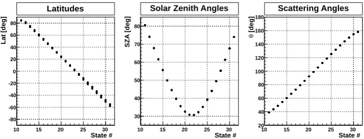
The data set used in this study was selected so as to facil-itate the comparison with the model data. First, 1 measure-ment orbit was chosen arbitrarily, from which 22 limb mea-surement sets (called states) with 4 profiles each and with a solar zenith angle (SZA) lower than 80◦ on the descend-ing node of the orbit were selected. This reference orbit is orbit 33750 from 13 August, 2008. The measurement time lines of SCIAMACHY cause a recurrence of the exact same viewing geometries of some of these 22 states in about ev-ery other orbit in the period between the 9 and 20 August for each year between 2004 and 2010, and also in a smaller set of data from mid-April of these years. Altogether, about 550 orbits were found where a minimum of 8 states matched the viewing geometries of the corresponding reference states. A state was called a match with the reference state if the solar zenith angles agreed within 0.1◦_{and the relative azimuth}

an-gles within 1◦_{for all tangent height steps. Before 2004 and}

after 2010 there are no matching states because the nominal execution of limb states was different then. Note that no par-ticular requirement was imposed on the location of the tan-gent point except for the exclusion of the Southern Atlantic Anomaly (SAA) region. Effectively this means that the view-ing geometry correspondview-ing to any given reference state is evenly distributed over all longitudes but covers only a very narrow latitude band. The average statistics for each refer-ence state per year varies between 20 and 50 for the August data. Figure 1 shows the latitudes, SZA and single scattering anglesθ for the described data set versus the state index of the reference orbit. Note that no explicit requirement was im-posed on the tangent height itself, in fact it varies randomly by a few hundred meters at each step. The selected data set al-lows a statistical analysis of data with the same measurement

2_{The polarization value from PMD 7 is not used operationally;}

(5)

State #

10 15 20 25 30

Lat [deg]

-80 -60 -40 -20 0 20 40 60 80

Latitudes

State #

10 15 20 25 30

S

Z

A

[

d

e

g

]

30 40 50 60 70 80

Solar Zenith Angles

State #

10 15 20 25 30

[deg]

θ

20 40 60 80 100 120 140 160 180

Scattering Angles

Fig. 1. Latitudes (left panel), SZA (middle panel) and single scattering angles for the data set used in this study vs. the state counter of the

reference orbit 33 750 (see text).

configurations but different atmospheric and surface condi-tions while reducing the number of different states to be sim-ulated by SCIATRAN to about 20. Version 7.03/7.04 of the operational Level 1b (L1B) data product was used to obtain the pixel and PMD signals, viewing angles, geolocation in-formation and auxiliary inin-formation from which the polar-ization values were then calculated. The algorithm applied is similar to, but not exactly the same as the one applied in the operational Level 0–1 processing. The changes to the polar-ization algorithm compared to the operational processor are described in Appendix A. Below 30 km the differences in the results between the operational and this algorithm are very small.

The radiometrically calibrated intensities were extracted from the L1B data using the scia nl1 tool (van Hees, 2012) for the application of the radiometric calibration. The applied calibration steps include the analog offset and limb dark cur-rent subtractions, nonlinearity correction in channel 6, inter-nal stray light correction, radiometric calibration with polar-ization correction and degradation correction. The memory effect correction in channels 1 to 5 was not applied.

3 SCIATRAN simulations

3.1 SCIATRAN

The specific viewing and scattering geometries of limb mea-surements require the solution of the vector radiative transfer equation (VRTE) in a spherical atmosphere to simulate the the radiance and polarization as measured by SCIAMACHY. For this study simulations are performed using SCIATRAN V3.1 (Rozanov et al., 2013). In SCIATRAN, the solution of the VRTE at each point along the line of sight is achieved by decomposing the Stokes vector of the diffuse radiation and the scattering matrix in each atmospheric layer into a Fourier series and then solving the equation for each Fourier com-ponent using the discrete ordinates technique. The single scattering contribution is integrated for each (spherical)

at-mospheric layer along the line of sight. To compute the multiple scattering contribution, the combined differential– integral (CDI) approach is applied (Rozanov et al., 2000). In this approach, the multiple scattering source function is cal-culated at a number of discrete points corresponding to dif-ferent solar zenith angles along the line of sight. At each of these points the diffuse radiation field is approximated by that of a pseudospherical atmosphere. This means that the trans-mission of the incident (solar) radiation is calculated within a spherically layered atmosphere, while the scattered radi-ation is calculated within a plane parallel atmosphere. The results for each discrete point are subsequently interpolated and integrated along the line of sight, in this way properly re-garding the curvature of the surface and atmospheric layers. In principle it is possible to repeat this calculation iteratively to arrive at a more accurate estimate of the top-of-atmosphere (TOA) reflectance (Rozanov et al., 2001). In SCIATRAN, this option is only available for the scalar mode; in the vec-tor mode it has not yet been implemented. Also, because of the computational effort it would not be feasible to run exten-sive model studies as the one presented here with the iterative scheme.

The vertical inhomogeneity of the atmosphere is mod-eled by dividing the atmosphere into homogeneous layers on a user-defined grid. Input profiles of pressure, temperature and, if desired, trace gas abundances and aerosol concentra-tions are interpolated to the middle between grid points to ob-tain a smoothly varying profile. Atmospheric refraction can be taken into account as well as the integration of the radi-ance over a vertical FoV. The surface reflection is modeled by a Lambertian albedo or by a bidirectional reflectance dis-tribution function (BRDF). The input to SCIATRAN is a set of line-of-sight and solar zenith angles and the relative az-imuth angles between the line of sight and the solar direction at the TOA. The output is the Stokes vector at the TOA in units of radiance or solar irradiance.

(6)

errors of a few percent in the calculated reflectance above 30 km (Rozanov et al., 2002). An ongoing comparison be-tween SCIATRAN in the vector mode and two Monte Carlo VRTMs, SIRO (Oikarinen et al., 1999) and MYSTIC (Emde et al., 2010; Mayer, 2009), revealed that not only the re-flectance suffers from inaccuracies but also and in particular the polarization. The relative errors ofq can be larger than 10 % on occasions, even at tangent heights as low as 20 km. Inaccuracies generally increase with tangent height and with increasing contribution from multiple scattering or scattering at the surface. These results do not invalidate any of the con-clusions drawn here on the quality of the SCIAMACHY data as shown below; however, they demand further improvement of the model.

3.2 Scenarios

The TOA reflectance at any given wavelength depends on a variety of atmospheric and surface parameters, most of which are generally not or only approximately known. This leaves two options for a quality assessment as this one. One could pick a few data points at particular measurement times and locations for which the atmospheric composition is very well known; for instance, a cloudless scene over the ocean far from anthropogenic or natural pollution sources. This would yield a small, and likely highly biased, data set. With the large FoV of SCIAMACHY it will be very difficult, though, to positively exclude the presence of clouds. In addition, un-certainties in the description of the BRDF and optical aerosol properties arise. A study along the lines of this idea was per-formed with the result that even with strict selection filters yielding not more than a handful of data points, the vari-ability of the measured reflectance between the selected data points is too large to distinguish between radiometric calibra-tion errors and model parameter uncertainties. Typically, the measured intensities matched modeled ones to within 20 % at tangent heights below 30 km. The small number of data points did not allow for a systematic investigation of the polarization values.

The second approach, which will be followed here, is to generate simulations spanning a large parameter space that could in principle accommodate most of the situations, and then study the statistical behavior of the data with respect to this parameter set. This approach can help identify biases, but again will not help in identifying calibration errors on a few-percent level.

SCIATRAN simulations were performed for the first pro-file of 20 out of the 22 limb states3 with a large number of different atmospheric parameter settings. The surface re-flectance was simulated with a Lambertian albedo between 0 and 1. The aerosol profile was divided into three layers (boundary layer, tropospheric and stratospheric aerosol) with

3_{There were errors in the simulation of two states, which is why}

they are not used here.

different types of aerosol and different aerosol loads. The shape of the profile in each layer was fixed, while the aerosol optical depth (AOD) was varied. Any combination of layer AOD and aerosol type within the first three layers was al-lowed. The aerosol types used for each layer are mixtures of the basic types recommended in the WMO report (Deepak and Gerber, 1983; Bolle, 1986). Appendix B lists the details of the aerosol types and profiles used. All aerosol types were assumed to consist of spherical particles, and the correspond-ing phase matrix was calculated uscorrespond-ing Mie theory.

Pressure and temperature profiles were fixed to the US-Standard scenario (COESA, 1976). Every major trace gas absorber relevant for the considered spectral range (300– 1700 nm) was included in the simulation with a fixed profile using a climatological data base similar to that described in Haley et al. (2004) and McLinden et al. (2010). Absorption cross sections were taken from the HITRAN 2004 data base for line absorbers (Rothman et al., 2005) (O2, H2O, CO2)

and from measurements by the SCIAMACHY PFM satellite spectrometer for O3and NO2(Bogumil et al., 2003). The

im-pact of density and absorber profile variations on the simu-lated radiances and polarization has been studied; results are discussed in Appendix B.

It is obvious that not all the possible combinations of albedo, aerosol and atmospheric species can be considered to be realistic assumptions for the data sample studied here. In particular, some of the aerosol scenarios are extremely ex-aggerated compared to typically prevailing conditions. How-ever, the definition of extreme scenarios may help in under-standing the limits within which measurements are expected to fall. It is later possible to select specific scenarios that match the data to a first approximation and conduct a more refined comparison between data and model.

In addition to the described main simulation data set, two smaller sets were generated as control samples to allow an assessment of some of the model dependence. Each of these comprises a subset of the limb states and of the aerosol and albedo scenarios of the main sample. In addition, in the first set, the aerosol content in the fourth (mesospheric) aerosol layer is significantly increased and varied. In the other set, clouds of different types, cloud top height and optical depth were simulated. Both sets serve as control samples to study the model dependence of this comparison.

3.3 Simulation of SCIAMACHY reflectances and polarization values

(7)

) 0 I/I π log( -2 -1.5 -1 -0.5

TH [km])

0 10 20 30 40 50

R (375 nm)

SCIAMACHY SCIATRAN set 0 SCIATRAN set 1

q -0.3 -0.2 -0.1 0

TH [km]

0 10 20 30 40 50

PMD 1 q

) 0 I/I π log(

-2 -1 0

R (481 nm)

q

-0.3 -0.2 -0.1 0

PMD 2 q

) 0 I/I π log(

-3 -2 -1 0

R (655 nm)

08/2004

q

-0.3 -0.2 -0.1 0

PMD 3 q

) 0 I/I π log(

-3 -2 -1 0

R (870 nm)

q(u)

-0.6 -0.4 -0.2 0

PMD 4(7) q(u)

q u

) 0 I/I π log(

-4 -3 -2 -1 0

R (1555 nm)

q

-0.5 0 0.5

PMD 5 q

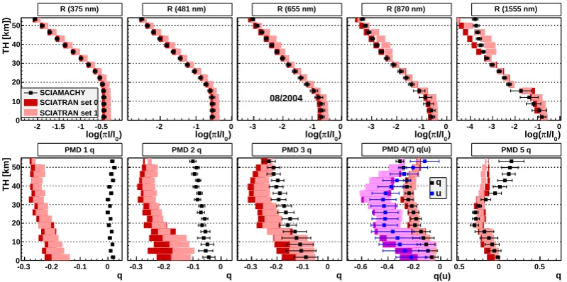
Fig. 2. Reflectance (top panel) and polarization profiles (bottom panel) for SCIAMACHY data (points) and SCIATRAN (boxes, red for

q, magenta foru); the shading indicates different simulation sets (see text for detail). The data set is for the reference state 20 (θ=92◦, SZA=32◦) in mid-August 2004. The polarization at 850 nm (4th panel) contains bothqanduvalues from PMDs 4 (black points) and 7 (blue points), respectively.

this approach would be impractical. Rather, the simulation was optimized for the validation of the SCIAMACHY limb polarization data by assuming

hqi_PMD≡q(hλPMDi) , (10)

where the average wavelengths of the PMD measurements

hλPMDiwere determined in studies with simulated high- and

medium-resolution spectra of the Stokes vector components. These studies showed that there is indeed a good, though tangent-height-dependent, correlation between the polariza-tion at an appropriately chosen wavelength and the effective polarization corresponding to the PMD measurements. The approximate error arising from this approach amounts to less than 0.01 with a small polarization-dependent component that can in principle be corrected for. For PMD 1, where the polarization drops rapidly between about 300 nm to a mini-mum around 350 nm and then slowly recovers, these differ-ences can be mitigated by choosinghλPMDi to be 375 nm,

while for the other PMDshλPMDi is about the value noted

in Table 1. In order to reduce the sensitivity to absorption features, the simulated wavelength for PMD 5 was set to 1556 nm, just outside the CO2absorption band. Concerning

PMD 5 it should also be noted that emission from the O21

and CO2 bands cannot be simulated by SCIATRAN. The

contribution from emission becomes relevant above 20 km and dominates the PMD signal above 30 km. As the emis-sion is unpolarized, the measured polarization should there-fore be significantly diluted compared to the simulations. For the comparison of the radiances, a few additional wave-lengths were selected, taking care that they are outside strong or highly variable absorption.

The TOA radiances were averaged over the vertical extent of the FoV of 0.045◦. Atmospheric refraction was not taken into account for this study.

4 Results

4.1 Reflectance and polarization profiles

Figure 2 shows profiles of the average reflectance R=

π I /I0,I0 being the solar irradiance, at 5 wavelengths

(cor-responding to the PMD 1 to 5 measurements) and of the av-erage of the retrieved fractional Stokes componentsq(from PMDs 1 to 5) andu(from PMD 7). The example is for one particular viewing geometry corresponding to one of the ref-erence limb states. The data are from August 2004; the av-erage single scattering angle ishθi =92.2◦at a solar zenith angle of about 32.4◦. At the single scattering angle around 90◦ high average polarization values can be expected. The small solar zenith angle, on the other hand, implies some variability at the longer wavelengths due to the high sensi-tivity to surface reflectance and tropospheric conditions. The model expectation is plotted as the reddish boxes, their width indicating the variance of the simulated data.

The expected model polarization values and their vari-ance were derived from the model in the following way: a subset of SCIATRAN simulations was selected by requiring

(8)

distribution of the data points, with a margin of 10 % added on both sides to account for possible systematic calibration errors. From the SCIATRAN subset obtained this way, two-dimensional distributions ofq vs.R andu vs.R were de-rived (see also Fig. 4 below) for each tangent height. From this two-dimensional histogram a one-dimensional distribu-tion was selected in a narrow slice around the measured re-flectance of each individual data point. The expected model polarization value was then estimated as a random value drawn from a Gaussian distribution with the mean and stan-dard deviation of the one-dimensional histogram. The aver-age expected polarization at a given tangent height should then amount to the mean of all model polarization values for all data points, with its variance taking into account both the variance in the reflectance of the data and the intrinsic spread of the model at a given reflectance. This procedure was performed independently for each wavelength and each tangent height, i.e., correlations between wavelengths were not considered.

The modeled average reflectance and its spread were sim-ply derived as the mean reflectance and variance of the SCI-ATRAN subset at each tangent height. Note that the aver-age reflectance of the model simulations is biased toward high values, although individual scenarios do yield lower re-flectances in many cases, ensuring that the data range is well covered. The model distribution was derived for two distinct SCIATRAN setups, where the first, dubbed “set 0”, is the basic set described in Appendix B containing only aerosols up to 35 km and the second, “set 1”, has added clouds in the troposphere as well as increased aerosol in the mesosphere. The difference between the simulation sets becomes visible in the average reflectance and polarization at tropospheric and mesospheric tangent heights. In general, the addition of clouds results in slightly higher average radiances and more depolarization at all tangent heights.

Qualitatively, the measured reflectances below about 30 km behave as expected: at tropospheric heights there is increasing variability with wavelength, while there is less variability at all wavelengths in the stratosphere. Above 30– 40 km the data tend to be significantly higher than the ba-sic (set 0) simulations. This behavior is geometry and wave-length dependent and can at least partially (below 50–60 km) be explained by the addition of aerosol in the mesosphere, as simulated in set 1.

Concerning the polarization, the obvious discrepancy be-tween model and data at UV-VIS wavelengths is striking. Aside from that, below about 40 km (25 km for PMD 5), the shape of the profile and the variability of the data seems to be well represented in the model for PMDs 2–5 and 7. The modeled variance for PMD 1 is too large. This is possi-bly a consequence of the simulation being only for a single wavelength rather that the average over the complete PMD range with a tangent-height-dependent spectral shape. The zig-zag pattern observed in PMD 1 and 2 is real and origi-nates from the alternating ASM mirror positions at each new

tangent height step, which is inherent in the limb scan pattern of SCIAMACHY.

Above 40 km, the SCIATRAN simulations become in-creasingly unreliable due to the above-mentioned limitations in approximating the spherical geometry (see Sect. 3.1). On the other hand, the data receive a larger contribution from spatial stray light at high altitudes. An assessment of data quality above ∼40 km can therefore only be inconclusive. The apparent offset between simulations and data for PMDs 1 to 3 in the stratosphere, however, cannot be explained by ei-ther stray light or model inaccuracies and variance. From the ongoing model intercomparison with Monte Carlo models, it is known that SCIATRAN has a tendency to predict too high depolarization at high altitudes, thus making the difference to the data even more manifest.

4.2 Variation with viewing geometry

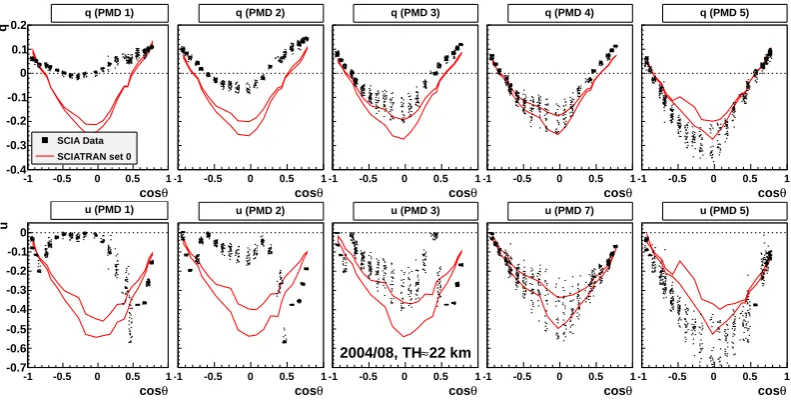
The fractional Stokes parametersqanduare plotted in Fig. 3 for the same data set (August 2004), this time using all refer-ence states, at a tangent height of TH≈22 km. The simulated data are derived in the same manner as described above. This plot shows that the observed offsets follow a defined pattern along a typical SCIAMACHY orbit. The results are plotted against the cosine of the single scattering angle that for this particular data set is a unique identifier for each limb profile, but keep in mind that for each single scattering angle there is also a unique solar zenith angle and latitude. For a large range of scattering angles, the polarization values are way too small at wavelengths below 850 nm, and too large above 1500 nm. It should be mentioned that the contribution from emission expected for the PMD 5 measurement would lead to a depolarization rather than too large polarization. Note that theuvalues for all PMDs but PMD 4 and 7 are derived from the theoretical assumption Eq. (8), i.e.,u=q·uSS/qSS.

Since the values forqderived from PMD 1 to 3 are too small or very close to zero,u consequently is too small as well. There are also features at cosθ≈0.5 and−0.8 at which the theoretical assumption completely fails becauseqSS≈0.

It can therefore be concluded that the polarization val-ues as well as the polarization correction in the radiomet-ric calibration of the UV-VIS spectra are highly inaccurate for a large range of wavelengths, scattering geometries and tangent heights.

4.3 Correlation between polarization and reflectance

(9)

θ cos -1 -0.5 0 0.5 1

u

-0.7 -0.6 -0.5 -0.4 -0.3 -0.2 -0.1 0

u (PMD 1) θ cos -1 -0.5 0 0.5 1

q

-0.4 -0.3 -0.2 -0.1 0 0.1 0.2

q (PMD 1)

SCIA Data SCIATRAN set 0

θ cos

-1 -0.5 0 0.5 1

u (PMD 2)

θ cos

-1 -0.5 0 0.5 1

q (PMD 2)

θ cos

-1 -0.5 0 0.5 1

u (PMD 3)

22 km ≈ 2004/08, TH

θ cos

-1 -0.5 0 0.5 1

q (PMD 3)

θ cos

-1 -0.5 0 0.5 1

u (PMD 7)

θ cos

-1 -0.5 0 0.5 1

q (PMD 4)

θ cos

-1 -0.5 0 0.5 1

u (PMD 5)

θ cos

-1 -0.5 0 0.5 1

q (PMD 5)

Fig. 3. Values forqandufrom the SCIAMACHY data of August 2004 (black points) for each PMD and from SCIATRAN simulations (red lines depicting the 1σ envelope of the expected distribution around the mean) at TH≈22 km.

in reflectance due to the surface or aerosol is much larger than the associated change in theQandU components of the Stokes vector, resulting in an effective depolarization. Eventually, the values will saturate when the optical thick-ness along the light path becomes large. The longer the wave-length, the larger the impact of aerosol and surface scattering on both the reflectance and the polarization should be. If the observed discrepancies were due to deficiencies in the mod-eling of the state of the atmosphere, for instance due to the assumption of Mie scattering on spherical aerosol particles, it should be therefore seen most clearly at the NIR wave-lengths.

In Fig. 4, the correlation betweenq and reflectanceR is shown for the same data as in Fig. 2 at a tangent height of about 22 km. The variability in the SCIATRAN data is due to variations of both the stratospheric aerosol load and tro-pospheric and surface parameters. There seems to be a sat-uration of the depolarization at high reflectance values. In the SCIAMACHY data, while being well correlated, this re-lationship does not follow the expected distribution. Even if adding ever more tropospheric or stratospheric aerosol would lead to stronger depolarization in the UV-VIS region, it would do even more so in the NIR region yielding polar-ization and reflectance values inconsistent with the measure-ments. It seems unlikely then that the observed differences can be explained by inadequate model simulations.

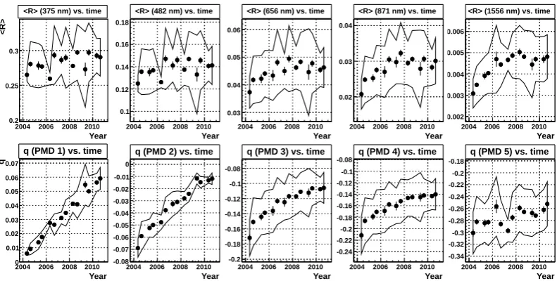
4.4 Long-term time dependence

SCIAMACHY was launched in March 2002 and has ever since experienced a degradation of its scanners and detec-tors. The throughput loss has been monitored using solar ob-servations along varying instrumental light paths. A large part of it can be explained by the deposition of dirt onto

the ASM and ESM mirrors, while a minor part can be at-tributed to changes in some parts of the optical bench (Snel and Krijger, 2009). To account for the degradation, the con-cept ofmfactors (Bramstedt et al., 2009) has been employed in which the measured pixel signals are corrected by a

fac-torm(t )=IS(t )/IS(t0). Here,IS is the solar radiance or

ir-radiance from the appropriate monitoring measurement at a given timet and the ratio is determined with respect to a reference timet0 close to the beginning of stable

instru-ment operations. Themfactors correct for a major part of the degradation effects, but they cannot cover for their scan an-gle and polarization dependence. The relative degradation of the PMDs compared to the science channels is taken care of by the time dependence of the in-band signal that is obtained from the ratio of the virtual sum (cf. Eq. 6) to the PMD signal in measurements of the solar irradiance and that is updated on a daily basis. The monitoring of the polarization sensitiv-ity is not possible with the monitoring measurements, which are all based on unpolarized input.

(10)

Fig. 4. Correlation between polarizationqand reflectanceR, for the same data as in Fig. 2 (August 2004, reference state 20, TH≈22 km).

Year

2004 2006 2008 2010

<R>

0.2 0.25 0.3

<R> (375 nm) vs. time

Year

2004 2006 2008 2010

q

0 0.01 0.02 0.03 0.04 0.05 0.06 0.07

q (PMD 1) vs. time

Year

2004 2006 2008 2010 0.1

0.12 0.14 0.16 0.18

<R> (482 nm) vs. time

Year

2004 2006 2008 2010 -0.08

-0.07 -0.06 -0.05 -0.04 -0.03 -0.02 -0.01 0

Year

2004 2006 2008 2010 0.03

0.04 0.05 0.06

<R> (656 nm) vs. time

Year

2004 2006 2008 2010 -0.2

-0.18 -0.16 -0.14 -0.12 -0.1 -0.08

Year

2004 2006 2008 2010 0.02

0.03 0.04

<R> (871 nm) vs. time

Year

2004 2006 2008 2010 -0.24

-0.22 -0.2 -0.18 -0.16 -0.14 -0.12 -0.1 -0.08

Year

2004 2006 2008 2010 0.002

0.003 0.004 0.005 0.006

<R> (1556 nm) vs. time

Year

2004 2006 2008 2010 -0.34

-0.32 -0.3 -0.28 -0.26 -0.24 -0.22 -0.2 -0.18

Fig. 5. Time dependence of the average reflectance and polarization. Points with error bars represent the mean and its error, the envelope the

variance of the distribution. The data sample corresponds to the reference state 20, the average tangent height is 21.7 km. This plot contains both the April and August data samples.

exhibit a similar behavior, thus not revealing any significant scan angle dependence. Comparing with Fig. 4, the trends in the polarization are consistent with the trends in the re-flectance only for PMDs 4 and 5; for PMDs 1 to 3 they seem to be too large. That means that the observed trends cannot be explained with the simulated relationship between the mean reflectance and mean polarization alone. Of course, provided that the reflectance increase is really due to changes in atmo-spheric composition (albedo, cloud cover, aerosol), it can-not positively be excluded that in the UV-VIS region these changes “conspire” in way to generate trends in the polariza-tion along the vertical axis of Fig. 4. It is more likely that instrumental changes inside the OBM affecting the polariza-tion sensitivity can cause the observed depolarizapolariza-tion trends. Eventually, this ambiguity can only be solved by a rigorous analysis involving a retrieval of albedo and aerosol compo-sition combining all wavelengths and using more realistic model simulations. However, prior to that the large offset in the polarization values between model and data that have

ap-peared already at the beginning of life of the instrument has to be understood.

5 Error sources and in-flight recalibration

5.1 Assessment of error sources

The large spread in the model predictions, the uncertainties in the parameterization of the state of the atmosphere and the intrinsic model errors ofO(0.01)cannot explain the ob-served differences to the measured data. The remaining two other options are a failure of the polarization algorithm and errors in the calibration key data.

The initial inputs to the polarization algorithm are the PMD and the science detector signals weighted with the ra-tio of their throughputs and integrated over the PMD spectral range. Equation (6) can be rewritten as

IBS

P

V0

=

*

1+µP₂q+µP₃u

1+µD₂q+µD₃u

+

(11)

V0= X

i

S_iDM₁PD_,i . (11)

In the algorithm,q anduare assumed to be constant. Also, the numerator in the average term of Eq. (11) is usually dom-inating over the denominator, such that it is possible to ap-proximate

*

1+µP₂q+µP₃u

1+µD₂q+µD₃u

+

≈ 1+ hµ

P

2iq+ hµP3iu

1+ hµD₂iq+ hµD₃iu (12)

without changing the results noticeably. The averages of the MMEs,µ2,3, can be determined for each measurement as

hµP_n,Di = 1

V0

X

i

S_iDM₁PD_,iµ_niP,D, n=2,3. (13)

In particular, for the case of PMD 1 the denominator in Eq. (12) is very close to 1 within 1 % due to cancelations of positive and negative values ofµD₂_,₃, implying that

IBS

P

V0

−1≈ hµP₂iq+ hµP₃iu . (14)

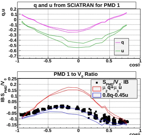
The black points in the bottom panel of Fig. 6 show the left-hand side (LHS) of this equation for PMD 1 as a function of the single scattering angle cosθ. Likewise, the red curve in this figure shows the expectation for the right-hand side (RHS) of Eq. (14) determined from the expectation values of SCIATRAN forqandu(magenta and green curves in the top panel) using the averageµi according to Eq. (13) from the

on-ground polarization key data. Clearly, neither the shapes nor the magnitude of the curves match.

The influence of each of the three calibration terms can now be examined separately. The in-band signal IB is essen-tially a scale factor for the relative calibration of PMD and science detectors. A change in the in-band signal by a factor

f close enough to 1 would first-order shift the entire curve by 1−f. On the other hand, a change in the major MME,

µP₂, would mainly scale the curve, while a change in in the minor MMEµP₃ would alter the shape of the curve propor-tional to the shape ofu. Assuming that the model values forq

anduresemble the true atmospheric polarization in a reason-able fashion, this figure shows that the sensitivities toqandu

of the PMD signal cannot be described with the averageµ2,3

determined from the on-ground key data. Reversely, it should be possible to “tune” the respective values in the SCIATRAN curve until it matches the data. This has been done for the blue curve in the bottom panel of Fig. 6 by changinghµP₂ito 0.8 andhµP₃ito−0.45 from their original values of 0.98 and

−0.11, respectively. The remaining small discrepancies may be due to a shift in the in-band signal, the contribution of the polarization to the integrated science detector signal and the above-mentioned intrinsic model errors.

From the above discussion it seems evident that the on-ground key data do not resemble the in-flight polarization sensitivities. A drastic change such as that observed in the

θ cos

-1 -0.5 0 0.5 1

q,u

-0.7 -0.6 -0.5 -0.4 -0.3 -0.2 -0.1 0 0.1

0.2 q and u from SCIATRAN for PMD 1

q

u

θ cos

-1 -0.5 0 0.5 1

0

/V

PMD

S

⋅

IB

-0.15 -0.1 -0.05 0 0.05 0.1 0.15 0.2 0.25

Ratio

0

PMD 1 to V

IB ⋅

0

/V

PMD

S u

3

µ q+

2

µ

0.8q-0.45u

Fig. 6. Top panel: expectation values forqandufor August 2004 data at TH≈21.7 km from SCIATRAN set 0; the curves depict the RMS around the mean value. Bottom panel: the points are the data for PMD 1 (LHS of Eq. 14) and the red curve represents the RMS around the expectation value of the RHS of this equation using av-erages of on-ground key data, while the blue curve represents the values obtained by settinghµP₂i =0.8 andhµP₃i = −0.4.

UV close to the beginning of life of the instrument can also not be explained by the rather gradual scanner degradation. A likely reason for the observed behavior is a phase shift within the optical bench of the instrument. A temperature-dependent phase shift in the predisperser prism that splits the beam and directs the light onto the individual detector channels and the PMDs had been observed already during the on-ground calibration measurements and is the main reason for the initial PMD sensitivity to 45◦ polarized light (Snel, 1999). This initialudependence is reflected in theµP₃, which is largest at UV wavelengths and then smoothly drops off. It is quite conceivable then that stress birefringence induced mechanically in flight by the lack of gravity or by temper-ature gradients within the instrument could have altered the initial polarization phase shift.

(12)

calibration measurements. A recent reanalysis using inde-pendent calibration data shows that the signs of some minor MMEs (e.g.,µD₃) may be wrong in some cases (Krijger et al., 2009).

The unexpectedly small PMD-to-detector signal ratios also explain the failure of the polarization algorithm, as seen in Fig. 3. Usingu/q=const.(Eq. 8), Eq. (14) can be solved forq:

q≈ 1

µP₂

IB S

P

V S0

−1 1+µ

P 3

µP₂

uSS

qSS

!

. (15)

A small value of the numerator would now automatically im-ply a small value ofq, and therefore a small value ofu. In the original Eq. (14), however, small values of the left-hand side can just as well be explained by a partial cancelation of both terms on the right-hand side. Without an absolute input value foru, the virtual sum equation will always yield a smallqif the contributions ofµP₂qandµP₃uare opposite and compara-ble, as is the case for most of the limb-viewing geometries of SCIAMACHY.

5.2 Recalibration of polarization sensitivity using in-flight data

The approach taken in the previous section to explain the measured PMD signals can be reversed to find the values for the MMEs that yield polarization values compliant with the expected ones from the model. Here, a method is presented that is to be considered a first step towards a recalibration of the polarization key data, thus providing information on the sensitivity of the data to these parameters and allowing to identify and address potential issues.

The same data set as described in Sect. 2.3 is used, and the matching SCIATRAN sets have been selected according to the method described in Sect. 4.1. That means, for each of the 14 independent data sets (one for April and August each year between 2004 and 2010), a corresponding SCIATRAN subset with the modeled intensities lying in the same range as the data at a given reference height was selected. From each such subset, histograms as shown in Fig. 4 were generated, separately for all of set 0 and set 1 (see Sect. 4.1 and Ap-pendix B), as well as for two subsamples of set 0 containing either stratospheric background or volcanic aerosol.

Similarly to the procedure explained in Sect. 4.1, a mean valueqS is determined for the model, and the difference

be-tweenqDataand the model expectation valueqSis minimized

by adjusting the three fit parameters IB,µP₂andµP₃. Details of the fit methods are explained in Appendix C. The fit was carried out for one tangent height step above the reference tangent height. The values for the MMEs obtained with this method thus correspond to the ones that make the data agree on average with the mean value of the model given the re-flectance for each measurement point. The advantage of this method compared to fitting the data on an individual profile basis is that at least some model uncertainties arising from

inappropriate parameter settings and profile shapes can be mitigated. A profile-by-profile fit would also require an iter-ative adjustment of the model similar to optimal estimation retrievals, which would be forbiddingly slow.

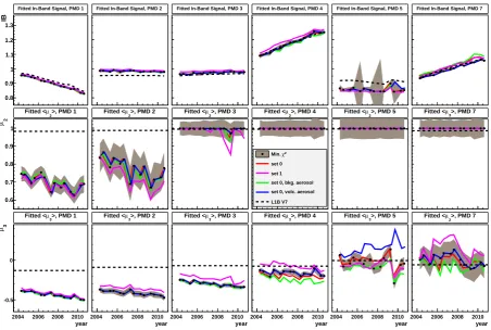
5.3 Preliminary results

Figure 7 shows the results for the three fit parameters. The fitted in-band signal is plotted in the top row. The colored curves show the results for the individual SCIATRAN sub-samples as described above; the black points with the gray shaded error band give, for each point in time, the result for the SCIATRAN sample with the lowestχ2and its error. This curve is shown only to give an impression on the associated intrinsic fit errors, not to make a judgment on the goodness of fit with respect to each subset. The dashed line shows the in-band signal derived from the solar measurements that is used in the operational Level 0–1 processor. The trend in this in-band signal is well captured by the fit. The observed off-sets, which are significant for all but PMDs 4 and 7, are by and large consistent with an independent analysis of nadir backscattering data atθ∼180◦_{. There is also some}

depen-dence on the chosen model subset that will have to be re-garded as a systematic fit error.

In the middle row the sensitivity to the major polarization component of the respective PMDs (i.e.,µP₂ for PMDs 1–5 andµP₃ for PMD 7) is shown, with the same coding for the individual curves. The dashed lines here indicate the mean values of the corresponding on-ground calibration key data. The intrinsic fit error on this MME is much larger, but it is still obvious that it differs significantly from the on-ground calibration data for PMD 1 and PMD 2, and exhibits a sig-nificant trend there. The difference between simulation sets is smaller than the fit parameter uncertainty, although the val-ues obtained from set 1 are systematically lower for PMD 1 and 2.

The fit results for µP₃ (PMD 1–5) and µP₂ (PMD 7) are shown in the bottom row, with the perhaps most surprising result that the sensitivities touin PMDs 1–3 are much larger than the initial on-ground measurements suggest. The model dependence is relatively large and increases with wavelength. A significant trend can be observed for PMDs 1 to 3 as well. As already discussed above, with this method it is not possi-ble to unambiguously decide whether these trends are caused by actual trends in the physical state parameters that are not captured by the model or by instrumental change. From the fact that the behavior of the fitted in-band signal agrees well with model-independent measurements, it can be concluded, though, that the trends are at least partially due to instrument degradation.

(13)

year

2004 2006 2008 2010

3

µ

-0.5 0

>, PMD 1 3 µ

Fitted <

2

µ

0.6 0.7 0.8 0.9 1

>, PMD 1 2 µ

Fitted <

IB

0.8 0.9 1 1.1 1.2 1.3

Fitted In-Band Signal, PMD 1

year

2004 2006 2008 2010

>, PMD 2 3 µ

Fitted < >, PMD 2 2 µ

Fitted <

year

2004 2006 2008 2010

>, PMD 3 3 µ

Fitted < >, PMD 3 2 µ

Fitted <

year

2004 2006 2008 2010

>, PMD 4 3 µ

Fitted < >, PMD 4 2 µ

Fitted <

2 χ Min. set 0 set 1 set 0, bkg. aerosol set 0, volc. aerosol L1B V7 Fitted In-Band Signal, PMD 4

year

2004 2006 2008 2010

>, PMD 5 3 µ

Fitted < >, PMD 5 2 µ

Fitted <

year

2004 2006 2008 2010

>, PMD 7 2 µ

Fitted < >, PMD 7 3 µ

Fitted <

Fig. 7. Results of the key data fits to SCIATRAN vs. time. Top panels: in-band signal for PMDs 1–5 and 7, middle panels:hµP₂ifor PMDs 1–5 andhµP₃ifor PMD 7, bottom panels:hµP₃ifor PMDs 1–5 andhµP₂ifor PMD 7. The black points with the fill area correspond to the values for best fitting SCIATRAN subset for each point in time and their errors. The colored curves are the results for the individual SCIATRAN samples and the dashed curve shows the values that are actually used in the Level 0–1 algorithm.

in the fit between genuine depolarization and cancelation of

µP₂qandµP₃uin the PMD signal. It is therefore likely that, for the cloudless scenes in set 0, the fit compensates the depolar-izing effects of actual clouds by increasing the magnitude of

µP₃ – and thereby decreasing the PMD signal. In addition to the obvious systematic differences between the results for set 0 and set 1, there may also be a small seasonal component in the fit parameters for PMDs 1 to 3, which could be related to a seasonal variation of cloud cover. Note, though, that the effect of clouds is overestimated by SCIATRAN, both due to the assumption of homogeneous layers and because of the aforementioned intrinsic model errors. The set 1 simulations are therefore not necessarily more realistic.

The fit residuals are wavelength and viewing geometry de-pendent, with the maximum values reaching from about 0.01 for PMD 1 to a few 10−2 for PMDs 2 to 4 to around 0.1 for PMD 5 and 7. This is about the expected range when regarding both model and measurement errors.

5.4 Discussion

The results presented here show that it is in principle possi-ble to recalibrate the polarization sensitivities using a model

for the expected polarization and in-flight data. In particular, the good representation of the in-band signal by the fit com-pared to the solar reference measurements as well as to nadir measurements (not shown here) indicate that even this very reduced data set used here has sufficient sensitivity to ex-tract information about the time-dependent behavior of the MMEs. The method can of course later be expanded to a more extended data set covering other seasons and more ge-ometries, yielding more independent combinations ofq and

(14)

The observed behavior of the MMEs, in particular the wavelength dependence ofµP₃, is indeed indicative of a polar-ization phase shift generated by the predisperser prism (Snel, 1999; Frerick, 1999). Important information about its mag-nitude and time dependence can be gained from these fit re-sults. Likewise, it should be possible to directly fit the phase shift rather than individual end-to-end MMEs by means of an instrument model as described in Snel and Krijger (2009) by adding a retarding element to it.

The results shown and discussed here are therefore to be considered a preliminary but useful step towards an in-flight recalibration of the polarization sensitivity of SCIAMACHY. They can as well serve the purpose of discussing the implica-tions for the polarization measurements and the polarization correction:

– First, the observed enhancement of the sensitivity tou

in the UV-VIS brings about an enhancement of the com-plications due to the polarization algorithm discussed in Sect. 5.1 (Eq. 15). That means, even if the true po-larization sensitivities were known with high accuracy, the current algorithm would still fail to give large po-larizations for bothq andu. The algorithm needs to be changed in order to provide a fixed estimate foru di-rectly to the virtual sum equation. The estimate can be based on assumptions such as Eq. (8), or, more appro-priate for the limb mode where the variability in this ratio is large, a model estimate from the relationship be-tweenuand the measured reflectance. The large sensi-tivity touimplies that the accuracy ofqwill be severely impacted by the uncertainty in the estimate foru.

– Another important issue to note is that the fit does not

actually deliver the polarization sensitivitiesµP₂_,₃of the PMDs but rather an effective combination of PMD and detector sensitivities4. From the fit alone, it is not possi-ble to derive the detector sensitivities separately. With-out an instrument model that can describe the observed changes in the effective polarization sensitivities, it is therefore not possible to derive the detector sensitivities needed for the polarization correction to the radiometric calibration. In particular, the effect on the nadir polar-ization measurements and calibration remains unclear. If the cause for the changes is a phase shift in the predis-perser prism, such an instrument model would be avail-able and could in principle be used to infer the phase shift directly from the fits. The Mueller matrix for each relevant light path and for both science detectors and PMDs can then be derived from the model (Snel and Krijger, 2009).

4_{Note that the correction for the initial values of the detector}

MME is contained in the factorcdin Eq. (C1). A systematic error

in these MMEs would therefore result in a systematic error on the fitted MMEs.

6 Conclusions

A rigorous study has been performed to assess the quality of the SCIAMACHY limb polarization measurements. Com-parison with SCIATRAN simulations revealed large discrep-ancies between model and data that are most prominent in the UV and visible regions. These discrepancies are outside the range of possible model uncertainties. In the UV, differences between measured and predicted polarization values amount to as much as 0.25 for q and 0.5 foru. There is a clearly systematic behavior with the viewing geometry along a typ-ical orbit. The discrepancies can be ultimately related to an instrumental change of the polarization sensitivities and, in addition, to a subsequent failure of the polarization algorithm to determine the correct polarization values. Erroneous or in-effective polarization corrections lead to errors in the abso-lute radiometric calibration of up to 15 %. Also, the spectral shape of the measured radiance may be impacted – for in-stance in the region around 350 nm, where the polarization sensitivity has some particular spectral features. The discus-sion here concentrated on the limb data; however, nadir data may be affected as well, albeit to a lesser extent.

The model can be used to recalibrate the effective polar-ization sensitivity of the instrument with in-flight limb data. Preliminary results indicate that it is possible to derive the relevant parameters from fits of the data to the model. The fit results reveal a dramatic shift of the in-flight polarization sen-sitivities compared to on-ground calibration measurements, hinting at a phase shift inside the instrument’s optical bench module as the likely cause. The accuracy of the fit needs to be further improved by extending the number of independent data points and reducing the sensitivity to model uncertain-ties. Alternative methods are currently being investigated.

Eventually, the results of this study and further in-vestigations will lead to an improved understanding of the instrument behavior and possibly a recalibration of the (time-dependent) polarization sensitivities. By adapting the polarization algorithm properly, the accuracy of the polarization data can be considerably improved.

Appendix A

Polarization algorithm details

The polarization algorithm uses Eq. (6). The pixel signals

Si are derived from the raw ADC counts delivered in the

(15)

key data used to calculate the MMEs are identical to the ones used in the operational processor. The MMEs are interpo-lated to the scan angles encountered in each measurement. Bad or dead detector pixels specified in a bad and dead pixel mask (BDPM) delivered with the L1B product are excluded from the virtual sum, and their values are replaced by an in-terpolation involving the adjacent good pixels.

The virtual sum equation is solved using the Brent root-finding algorithm. For PMDs 1–5 the assumption Eq. (8) is made for u if |q|>0.02. If |q|<0.02, u=cuSS with

c≈0.8. The value ofu is recalculated in each step of the iteration. If in an iteration stepq2+u2> q_SS2 +u2_SS,uis ad-justed tou= ±

q

q_SS2 +u2_SS−q2_{, with the sign fixed by the}

sign ofuSS. This strategy to adjustucauses the virtual sum to

have more than one solution in some cases in the nadir mode, from which only one (not necessarily the correct one) will be identified. There is no indication that this happens with limb data as well.

Below the differences of the algorithm used in this study and the operational L1B processor are listed.

– The polarization algorithm was applied to all tangent

heights. In the operational algorithm, above 30 km an extrapolation using the single Rayleigh scattering value is used.

– No memory effect correction was applied to the pixel

detector signals. The memory effect is a residual sig-nal from the previous exposure. During a step from one tangent height to the next in a limb scan, a pixel expo-sure is taken but not stored in the data, with the con-sequence that for the first exposure after each step no information on the previous signal is available. Instead, an interpolation between the signals at the two tangent heights is made. Due to a bug in the interpolation rou-tine of the processor, the memory effect was wrongly calculated for each first readout in a limb scan, leading to visible artifacts both in the limb radiance and the po-larization above approx. 40 km. As the memory effect is very small between 20 and 30 km and hardly changes anymore above 30 km, by omitting the memory effect correction these artifacts can be significantly reduced, while retaining radiometric accuracy.

– The PMD signals were filtered for spikes caused by

en-ergetic particles hitting the detectors. The frequency of these spikes is not very high outside the SAA region, but if they occur they can cause significant polarization errors above about 40 km. PMD 7 is the one affected most by spikes, followed by PMD 1. The efficiency of the filtering algorithm is not 100 % so that quite gener-ally above 55 km, the PMD 7 values can be considered unreliable.

– Similarly to the PMDs, also the science detector

pix-els can be hit by particles. In the operational processor

a check was implemented to identify hot pixels during the measurement of the limb dark signal at 250 km tan-gent height. This check was not implemented here, re-sulting in a slightly different limb dark signal subtrac-tion. Outside the SAA, hot pixels occur only rarely such that the impact on the virtual sum is minuscule.

– As mentioned above, bad pixels specified in the BDPM

are not used in the virtual sum. In channel 6 above 1585 nm a significant number of pixels suffers from a so-called random telegraph signal (RTS), which causes their dark currents to randomly jump between two or more different values. These pixels are not ne