www.atmos-meas-tech.net/6/2419/2013/ doi:10.5194/amt-6-2419-2013
© Author(s) 2013. CC Attribution 3.0 License.
Atmospheric
Measurement
Techniques
Ten years of MIPAS measurements with ESA Level 2 processor V6 –
Part 1: Retrieval algorithm and diagnostics of the products
P. Raspollini1, B. Carli1, M. Carlotti2, S. Ceccherini1, A. Dehn11, B. M. Dinelli3, A. Dudhia4, J.-M. Flaud5, M. López-Puertas7, F. Niro6, J. J. Remedios8, M. Ridolfi2, H. Sembhi8, L. Sgheri9, and T. von Clarmann10 1Istituto di Fisica Applicata “N. Carrara” (IFAC) del Consiglio Nazionale delle Ricerche (CNR), Firenze, Italy 2University of Bologna, Bologna, Italy
3Istituto di Scienza dell’Atmosfera e del Clima (ISAC) del Consiglio Nazionale delle Ricerche (CNR), Bologna, Italy 4Atmospheric, Oceanic and Planetary Physics, Clarendon Laboratory, Oxford University, UK
5Laboratoire Interuniversitaire des Systèmes Atmosphériques (LISA) CNRS, Univ. Paris 12 et 7, France 6SERCO SpA c/o European Space Agency ESA-ESRIN, Frascati, Italy
7Instituto de Astrofísica de Andalucía (CSIC), Granada, Spain
8Earth Observation Science, Department of Physics and Astronomy, University of Leicester, UK
9Istituto per le Applicazioni del Calcolo (IAC) del Consiglio Nazionale delle Ricerche (CNR), Section of Florence, Italy 10Karlsruhe Institute of Technology (KIT), Institute for Meteorology and Climate Research (IMK), Karlsruhe, Germany 11ESA-ESRIN, Frascati, Italy
Correspondence to: P. Raspollini ([email protected])
Received: 4 December 2012 – Published in Atmos. Meas. Tech. Discuss.: 15 January 2013 Revised: 15 July 2013 – Accepted: 5 August 2013 – Published: 23 September 2013
Abstract. The MIPAS (Michelson Interferometer for Passive
Atmospheric Sounding) instrument on the Envisat (Environ-mental satellite) satellite has provided vertical profiles of the atmospheric composition on a global scale for almost ten years. The MIPAS mission is divided in two phases: the full resolution phase, from 2002 to 2004, and the optimized res-olution phase, from 2005 to 2012, which is characterized by a finer vertical and horizontal sampling attained through a reduction of the spectral resolution.
While the description and characterization of the products of the ESA processor for the full resolution phase has been already described in previous papers, in this paper we focus on the performances of the latest version of the ESA (Eu-ropean Space Agency) processor, named ML2PP V6 (MI-PAS Level 2 Prototype Processor), which has been used for reprocessing the entire mission. The ESA processor had to perform the operational near real time analysis of the ob-servations and its products needed to be available for data assimilation. Therefore, it has been designed for fast, contin-uous and automated analysis of observations made in quite different atmospheric conditions and for a minimum use of external constraints in order to avoid biases in the products.
that minimum constraints are used and the best vertical res-olution obtainable from the measurements is achieved in all atmospheric conditions.
Random and systematic errors, as well as vertical and hor-izontal resolution are compared in the two phases of the mis-sion for all products, namely: temperature, H2O, O3, HNO3,
CH4, N2O, NO2, CFC-11, CFC-12, N2O5and ClONO2. The
use in the two phases of the mission of different optimized sets of spectral intervals ensures that, despite the different spectral resolutions, comparable performances are obtained in the whole MIPAS mission in terms of random and system-atic errors, while the vertical resolution and the horizontal resolution are significantly better in the case of the optimized resolution measurements.
1 Introduction
The Michelson Interferometer for Passive Atmospheric Sounding (MIPAS) is a limb-viewing Fourier transform spectrometer that sounded the emission of Earth’s atmo-sphere in the spectral range from 685 to 2410 cm−1on board the ESA (European Space Agency) Envisat (Environmental satellite) satellite (Fischer et al., 2008).
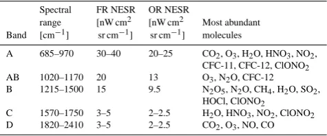
Its unique observation of the atmospheric emission has provided day and night and regularly spaced sampling that exhaustively characterizes the chemical and physical pro-cesses occurring in the atmosphere from 6 to 70 km altitude, for observations made in nominal mode, and up to 170 km for observations made in special modes. Table 1 summarizes the main characteristics of the MIPAS spectral bands with the in-dication of the main molecules emitting in each of them. The satellite was launched on 1 March 2002, and in the first two years of operation (from July 2002 to March 2004) MIPAS acquired, nearly continuously, measurements at full spectral resolution (full resolution (FR) measurements, characterized by the spectral sampling of 0.025 cm−1). On 26 March 2004 FR measurements were interrupted because of anomalies in the velocity of the interferometer drive unit of MIPAS and the analysis of instrument reliability and performance rec-ommended the use of a shorter interferometric sweep, corre-sponding to both a lower spectral resolution (0.0625 cm−1) and a shorter measurement time (1.8 s instead of 4.5 s). Test measurements with reduced spectral resolution were suc-cessfully performed in August/September 2004 and, accord-ingly, the reduction in the measurement time was exploited to make more frequent observations both in the vertical (limb) domain and in the horizontal domain (along the orbit).
With these changes, which provide, for the operational data products, an optimized compromise between spectral and spatial resolutions (optimized resolution, OR), MIPAS restarted operations on 9 January 2005 with a duty cycle shorter than 40 %. Since then, due to the recovering perfor-mance of the drive unit, the duty cycle was progressively increased until 1 December 2007 when a 100 % duty cycle
Table 1. MIPAS spectral bands: spectral range, NESR, most abun-dant molecules.
Spectral FR NESR OR NESR
range [nW cm2 [nW cm2 Most abundant Band [cm−1] sr cm−1] sr cm−1] molecules
A 685–970 30–40 20–25 CO2, O3, H2O, HNO3, NO2,
CFC-11, CFC-12, ClONO2
AB 1020–1170 20 13 O3, N2O, CFC-12
B 1215–1500 15 9.5 N2O5, N2O, CH4, H2O, SO2,
HOCl, ClONO2
C 1570–1750 3–5 2–2.5 H2O, HNO3, NO2, ClONO2
D 1820–2410 3–5 2–2.5 CO2, O3, NO, CO
was again attained. MIPAS was successfully operated with this full duty cycle until 8 April 2012, when an Envisat anomaly occurred resulting into the loss of communication between ground and satellite and the end of MIPAS observa-tions (ESA, 2012a).
MIPAS was one of the first Envisat instruments to be fully operational after the launch, providing very high qual-ity Level 1 and Level 2 products. The ESA operational near real time analysis provided from the very beginning vertical profiles of temperature and of volume mixing ratio (VMR) of H2O, O3, HNO3, CH4, N2O and NO2from pole to pole,
This paper is focused on the ESA processor that was used during the Envisat mission for both the near real time anal-ysis, whose requirement is the distribution of the products within three hours from the measurement time, and for the offline analysis, performed on consolidated Level 1 data, that benefits from a posteriori knowledge related to calibration, auxiliary data and precise orbit information. The capacity of operating in near real time made the MIPAS ESA dataset particularly suitable for the use in operational data assimi-lation systems. Indeed, near real time MIPAS ozone profiles were actively assimilated at the ECMWF (European Centre for Medium-Range Weather Forecasts) from October 2003 until the end of March 2004 (Dethof, 2003), and, after the in-terruption in 2004, from 8 December 2011 until 8 April 2012. The assimilation of MIPAS ozone data at the ECMWF was proven to substantially improve the quality of the ECMWF ozone analyses (Dragani, 2012; Thépaut et al., 2012), in par-ticular the good vertical resolution of MIPAS in the strato-sphere could provide a very useful constraint on the ozone analyses.
The description and characterization of the ESA proces-sor’s products of the full resolution phase was already de-scribed in Ridolfi et al. (2000) and Raspollini et al. (2006). In this paper we focus on the performances of the latest ver-sion of the ESA processor ML2PP (MIPAS Level 2 Proto-type Processor) V6, which has been used for reprocessing the entire MIPAS mission, i.e., including both phases. The com-plete ML2PP V6 database has been released in 2012 (ESA, 2012b), data access is provided via fast registration at https: //earth.esa.int/web/guest/data-access/browse-data-products.
The ML2PP V6 dataset contains the upgrades that were needed after the change of the operating mode in 2005 both in the algorithm, to cope with the finer altitude sampling of the OR measurements, and in the spectral intervals selected for each retrieval, to cope with the reduced spectral resolu-tion. Since the retrieval is performed at the grid of the mea-sured tangent altitudes and this grid is significantly finer, for the OR measurements, than the MIPAS instantaneous field of view (IFOV, 3 km) in the upper troposphere and lower stratosphere, the retrieval of the OR measurements resulted in an ill-conditioned problem and required a regularization approach that was not previously needed for the analysis of the FR measurements. Furthermore, in order to minimize the total error in the two phases of the mission, spectral intervals specifically optimized for each of them were used.
Even if the whole MIPAS mission has now been repro-cessed with the same algorithm, the different vertical and horizontal samplings and the different spectral intervals used in the two phases of the mission represent a discontinuity in the measurements whose impact on the products has been carefully investigated. This analysis is split in two parts. The first part, covered by this paper, makes an overview of the choices made for the inversion of the OR measurements starting from the retrieval approach designed for the FR mea-surements. The paper is then focused on the description of
the upgraded diagnostics used for the characterization of the Level 2 products and the comparison of the performances in the two phases of the mission in terms of random and system-atic errors and spatial resolution. The second part, covered by a companion paper (Raspollini et al., 2013), will study whether the discontinuity in MIPAS measurements in the two phases has an impact on the bias of the products between the two phases of the mission.
2 Characteristics of the two phases of the MIPAS mission
In both phases of the mission different measurement modes are used to observe different processes in the atmosphere with either better sampling or better altitude coverage. Cor-responding modes in the two phases of the mission are meant to achieve the same scientific objectives but may slightly dif-fer for the altitude coverage and for the altitude grid. The general objectives of the different measurement modes are shortly reviewed.
The nominal mode (NOM) is the basic mode used to study chemistry and transport and to provide a database for clima-tology, trend analyses and near real time applications. It is designed to cover the upper troposphere, the stratosphere and the lower mesosphere (approximated boundaries 6–70 km).
The upper troposphere–lower stratosphere (UT–LS) mea-surement mode, called UTLS-1, is tailored to studies of at-mospheric processes in the UT–LS region (including the tropical tropopause layer). It provides a trade-off between vertical and horizontal resolution as well as vertical cover-age, ensuring a fine vertical and along-track sampling be-tween the upper troposphere and the middle stratosphere.
The middle atmosphere (MA) mode covers most of the stratosphere, the mesosphere and the lower thermosphere (from 18 to 102 km). This mode is dedicated to studying linkages between the upper atmosphere and the stratosphere, i.e., the global circulation and transport of CO and NOx
from the mesosphere down to the stratosphere in polar win-ter hemispheres, as well as solar proton events affecting both the upper atmosphere and the stratosphere. This mode is also used to monitor the quality of operational retrievals that neglect deviations from local thermodynamic equilib-rium (non-LTE).
The upper atmosphere (UA) mode covers all the meso-sphere and the lowest part of the thermomeso-sphere and is mainly dedicated to measurements of high-altitude NO and temperature.
Table 2. Characteristics of FR and OR measurements for the most used measurement modes of the two phases of the mission.
FR measurements (from June 2002 to March 2004) Spectral resolution: 0.025 cm−1
Measurement mode Horizontal sampling No. of scans Vertical sampling
NOM 550 km 17 3 km step 5 km step 8 km step
6–42 km 42–52 km 52–68 km
OR measurements (from January 2005 to April 2012) Spectral resolution: 0.0625 cm−1
Measurement mode Horizontal sampling No. of scans Vertical sampling
NOM 410 km 27 1.5 km step 2 km step 3 km step 4 km step 4.5 km step
6–21 km 21–31 km 31–46 km 46–62 km 62–71 km
UTLS-1 290 km 19 1.5 km step 2 km step 3 km step 4.5 km step
8–21.5 km 21.5–27.5 km 27.5–33.5 km 33.5–51.5 km
MA mode 430 km 29 3 km step
18–102 km
UA mode 375 km 35 3 km step 5 km step
42–102 km 102–172 km
returned to the 100 % duty cycle, regular observations were made with a period of 10 days, consisting of 8 days of NOM mode measurements, 1 day of MA mode and 1 day of UA mode.
In OR measurements, NOM and UTLS-1 modes are characterized by a floating-altitude measurement grid. This means that the limb sounding grid is shifted rigidly with the lowest measured altitude t varying with the latitude,
θ, according tot=A+Bcos(2θ )−Ccos(90◦−abs(θ )). In this equationA=12 km,B=0 andC=7 km for the NOM mode andA=8.5 km,B=3 km andC=0 for the UTLS-1 mode. The floating-altitude sampling grid is meant to fol-low roughly the tropopause height along the orbit with the requirement to collect at least one spectrum within the tropo-sphere while avoiding too many spectra affected by clouds.
For a detailed description of all measurement modes used in the two phases of the mission see also Oelhaf (2008), while for a detailed calendar of MIPAS measurements see Dudhia (2008).
The MIPAS ML2PP V6 dataset covers all described mea-surement modes, although MA and UA modes are analyzed by the ESA processor only up to 70 km, since above this alti-tude the impact of LTE cannot be neglected and non-LTE effects are not handled in the forward model of the ESA processor. Analysis of MA and UA modes on the full altitude range are performed with the IMK-IAA algorithm (García-Comas et al., 2012; Bermejo-Pantaleon et al., 2011), while the analysis of UTLS-1 mode with IMK processor is described in Chauhan et al. (2009).
3 Upgrades in the code
The measurements of the first phase of the MIPAS mission were originally reprocessed by the ESA Instrument Process-ing Facilities (IPF) V4.1 and V4.2, based on the Optimized
Retrieval Model (ORM) code described in Ridolfi et al. (2000) and in Raspollini et al. (2006). These measurements were also validated with respect to correlative measurements (Ridolfi et al., 2007; Cortesi et al., 2007; Wang et al., 2007; Payan et al., 2009; Wetzel et al., 2007, 2013, all contained in a MIPAS Special Issue, 2006).
The main features of the algorithm originally designed for the analysis of the FR measurements are as follows.
1. Use of microwindows (MWs), i.e., selected spec-tral intervals containing relevant information on tar-get parameters and minimizing the systematic errors, which arise chiefly from approximations in the for-ward model and instrument errors (Dudhia et al., 2002; von Clarmann and Echle, 1998).
2. The forward model computes the radiative transfer integral properly taking into account the atmospheric vertical inhomogeneities but assuming homogeneity in the horizontal direction. Atmosphere is assumed to be in LTE and in hydrostatic equilibrium. The characteristics of the instrument (instrument line shape (ILS) and IFOV) are accurately modeled. The impact of unaccounted atmospheric effects (non-LTE, interfering species, etc.) is minimized through the MW selection. Scattering is not included in the radiative transfer integral, and the spectra affected by thicker clouds, identified by the cloud filtering algorithm (Spang et al., 2002, 2004; Raspollini et al., 2006), are not included in the analysis.
4. For each scan, sequential retrieval of the target species is performed (first H2O, then O3, HNO3, CH4, N2O
and NO2) after the simultaneous retrieval of the
pres-sure corresponding to the tangent altitudes and the re-lated temperature values (pT retrieval).
5. MW-dependent continuum absorption cross-section profiles and MW-dependent, but height-independent offset calibration values are jointly retrieved with ei-ther VMR or pT retrieval.
6. Initial guess of the target species is determined us-ing the profiles retrieved in the previous scan of the orbit appropriately combined with climatological and ECMWF profiles (if available).
7. Assumed profiles of the interfering species are given, whenever available, by the profiles retrieved in the vious retrievals (either the previous scan or the pre-vious retrievals of the same scan) appropriately com-bined with climatological and ECMWF profiles (if available).
8. Global fit analysis (Carlotti, 1988) is performed, con-sisting of the simultaneous fit of the whole limb scan-ning sequence of the spectra acquired at different tan-gent altitudes.
9. Nonlinear least squares fit is used with the Levenberg– Marquardt minimization and regularizing method (Levenberg, 1944; Marquardt, 1963; Hanke, 1997). In the following sections, the main changes to the re-trieval algorithm are described relative to the algorithm for FR measurements reported in Ridolfi et al. (2000) and in Raspollini et al. (2006). These include the adaptations to the Levenberg–Marquardt method, already utilized in the origi-nal FR algorithm, to avoid the ill-conditioning of the retrieval approach and an a posteriori self-adapting Tikhonov regu-larization technique. Diagnostics of the products specifically studied for the regularizing Levenberg–Marquardt method is also included as well as upgrades to the auxiliary data. Fi-nally, new products are described.
3.1 The regularizing Levenberg–Marquardt method
The ESA processor, being specifically designed for the near real time analysis of MIPAS measurements, had to be capa-ble of operating in an automatic way for a long period. These requirements, together with the choice of making a minimal use of external constraints in order to avoid biases in the re-trieved profiles, guided our design of the retrieval approach.
Letybe them-dimensional vector of observations with er-ror covariance matrix Syandf(x)the forward model, a
non-linear function of then-dimensional atmospheric state vector x. Due to nonlinearities, the problem is solved in a context of Newtonian iterations wheref(x)is linearized:
f(x)=f(xi)+Ki(x−xi), (1)
withi index of iteration and Ki Jacobian matrix ∂∂xf
calcu-lated at the linearization pointxi. The least squares solution
of the inverse problem minimizes the cost function:
χ2=(y−f(x))TS−y1(y−f(x)). (2)
Minimization ofχ2leads to the Gauss–Newton iteration:
xi+1=xi+
KiTS−y1Ki −1
KiTS−y1(y−f(xi)). (3)
In our application we modify Eq. (3) exploiting the Levenberg–Marquardt (Marquardt, 1963; Levenberg, 1944) method:
xi+1=xi+
KiTS−y1Ki+αiDi −1
KiTS−y1(y−f(xi)), (4)
where Di is chosen to be a diagonal matrix with elements
equal to those in the diagonal of KiTS−y1Ki. Considering that
the elements of the state vector are not homogeneous, this approach allows us to provide a correction that is scaled with the error of each element.
The parameter αi is adjusted according to a damping–
undamping strategy, see e.g., Lampton (2004). The iterations start with a smallα0. At each iteration, if the new statexi+1
provides a reduction of the chi-square (χ2(xi+1) < χ2(xi)),
thenxi+1is accepted andαi+1is selected such thatαi+1< αi. If the state xi+1 provides an increase of the chi-square
(χ2(xi+1) > χ2(xi)), thenxi+1is rejected and the iteration
is repeated with a larger value of αi. The iteration is per-formed until a final iteration criterion is fulfilled (see below). The Levenberg–Marquardt method has two distinct ef-fects. The first effect is the reduction of the correction ap-plied to the state vector at each iteration, while the correction vector itself is rotated from the Gauss–Newton step direction obtained from Eq. (4) withαi=0 towards the opposite
direc-tion of the gradient ofχ2(x), i.e., the steepest descent direc-tion. It follows that, with a large enoughαi, theχ2of the
it-erates monotonically decreases. By reducing the step length, the Levenberg–Marquardt method avoids making a too large correction, taking the solution outside of the linear approxi-mation range.
The second effect, that has been highly exploited for the analysis of the OR measurements due to the increased ill-conditioning of the retrieval problem, is that the inversion of the possibly ill-conditioned matrix KiTS−y1Ki is avoided
and replaced by the inversion of the matrix KiTS−y1Ki+ αiDi, which is better conditioned. This is particularly
The regularizing Levenberg–Marquardt method is, accord-ing to Hanke (1997), a semiconvergent method. Since the regularizing effect decreases with the number of iterations, the noise error increases, and the iterates may not converge in thexspace.
The final iteration criteria of the Levenberg–Marquardt it-erations should be implemented taking into account two con-flicting requirements. On one hand we must avoid stopping the iterations too early, with values ofχ2 too far from the minimum. On the other hand, the iterations must be stopped before the noise error becomes too large.
In the literature mentioned above, the consistency crite-rion is favored as a final iteration critecrite-rion, i.e., the iteration is stopped as soon as theχ2 is only slightly larger than its expected minimal value of 1. For MIPAS this criterion can-not be applied because we do can-not have a reliable expectation value for the minimum of the reducedχ2as a consequence of the variability of the systematic errors.
Instead, we use dedicated final iteration criteria.
The Level 2 processor originally used for the analysis of the FR measurements terminated the retrieval iterations (see Raspollini et al., 2006) when at least one of the following two conditions was fulfilled.
1. The relative difference between the actual χ2and its predicted value in the assumption of the linear forward model is smaller than a predefined thresholdt1.
2. The maximum inter-iteration relative correction to the target profile vector is less than a predefined threshold
t2.
In ML2PP V6, the final iteration criteria have been further improved in order to better handle the conflicting require-ments in the case of the ill-conditioned retrievals encountered with OR observations. In particular, in ML2PP V6 the condi-tion (1) on the relative difference betweenχ2and linearχ2, being a necessary, but not sufficient, condition to guarantee that a local minimum has been reached, is checked only if the actualχ2is less than a predefined thresholdt5.
Further-more, two other conditions have been added, the fulfillment of one of the four being sufficient to stop the retrieval. The two additional conditions are as follows.
3. The relative inter-iteration change of χ2 is less than a threshold t3. This condition is checked only if the actualχ2is less than the thresholdt5.
4. Then-dimensional state vectorxi at the current
itera-tion (i) is compatible with the state vectorxi−1at the
previous iteration, within a fractiont4of its error bars
represented by the covariance matrix Si (see Eq. 7). s
(xi−xi−1)TSi−1(xi−xi−1)
n < t4 (5)
The two newly added final iteration criteria allow to reduce, on average, the number of iterations by 18 %, while the re-sulting average χ2 does not increase. The average number of iterations for pT retrieval is about 4, while it is on aver-age about 3–3.5 for the other retrievals with the exception of NO2, for which the number of iterations is generally 1 or 2.
Both the chosen thresholds and the fact that the iteration is stopped when one of the final iteration criteria is fulfilled ensure that iterations not achieving a significative reduction of theχ2are avoided. Because of the ill-conditioning, fail-ing to stop the iterations may produce an unwanted increase of the noise error in the solution, and may result in oscillat-ing profiles. On the other hand, slightly oscillatoscillat-ing profiles due to ill-conditioning guarantee that a weak constraint has been used and are therefore tolerable, also considering that the adaptive a posteriori regularization will reduce these os-cillations (see Sect. 3.3).
3.2 Diagnostics of the Levenberg–Marquardt solution
In ill-conditioned retrievals the Levenberg–Marquardt solu-tion depends, to some degree, on both the initial guess of the state vector and the pathway followed by the iterative mini-mization procedure. The same dependence exists also for the covariance matrix and the averaging kernels (for their defini-tion see Sect. 4.2) of the Levenberg–Marquardt soludefini-tion.
For a proper calculation of the covariance and averag-ing kernel matrices of the Levenberg–Marquardt solution, ML2PP V6 uses an algorithm (Ceccherini and Ridolfi, 2010) in which all the retrieval iterations and the Levenberg– Marquardt damping are rigorously taken into account. This is particularly important in the retrieval of OR measure-ments, since, due to the ill-conditioning of the problem, the Levenberg–Marquardt parameter can be significantly differ-ent from zero.
To summarize the equations used, let i be the iteration count andcits value at convergence. Fori=0, . . . , c, we de-fine the sequence of gain matrices:
(Ti)j k≡ ∂(xi)j
∂yk
. (6)
With this definition, the covariance Scand the averaging
ker-nel Acmatrices of the Levenberg–Marquardt solutionxcare
given by
Sc=TcSyTTc, (7)
Ac=TcKc. (8)
Matrices Ti can be obtained by deriving the Levenberg–
Marquardt iterative formula (Eq. 4). Considering that the initial guessx0does not depend on the observationsy, we
T0=0
Ti+1 =
KiTS−y1Ki+αiDi −1
KiTS−y1+
+
I−KiTSy−1Ki+αiDi −1
KiTS−y1Ki
Ti.
(9)
It can be easily shown that in well-conditioned retrievals reaching the exact numerical convergence the covariance and the averaging kernel matrices calculated with Eqs. (7), (8) and (9) coincide with those calculated assuming the last iteration as a Gauss–Newton iteration (αc=0). On the
other hand, in ill-conditioned retrievals and/or in retrievals stopped with a physically meaningful final iteration crite-rion, the Levenberg–Marquardt solution and its diagnostic tools deviate from those predicted by the Gauss–Newton for-mulas. Additional tests and discussions on this algorithm can be found in Ceccherini and Ridolfi (2010). The use of this procedure ensures that in ML2PP V6 both covari-ance and averaging kernel matrices are properly computed even when the Levenberg–Marquardt procedure terminates with a Levenberg–Marquardt parameter significantly differ-ent from zero.
3.3 A posteriori regularization
As noted in Sect. 3.1, the profiles retrieved using only the Levenberg–Marquardt regularization often exhibit unphysi-cal oscillations. In the Level 2 ESA processor ML2PP V6 these oscillations are damped with a Tikhonov (Tikhonov, 1963) regularization scheme applied, a posteriori, to the Levenberg–Marquardt solution. The expression for the a pos-teriori regularized solution is
x=S−c1+λR
−1
S−c1xc+λRxa
. (10)
The regularization matrix R is obtained using the first deriva-tive operator, andxais an a priori profile, which, in our case,
is the null vector. This type of regularization is also used by the MIPAS IMK scientific processor (von Clarmann et al., 2003b, 2009b), but contrary to their approach, where the reg-ularization is performed during the iterations and the same regularization strength λ is used for all profiles, the ESA processor performs the a posteriori regularization and deter-mines, for each profile, the optimal regularization strength
λ on the basis of the so-called error consistency method, first introduced in Ceccherini (2005). This method selects the scalarλon the basis of the requirement that the regularized and un-regularized profiles should be compatible within the random error of the regularized profile, adapting its strength on the basis of the measurement error. This criterion leads to an analytical formula for the calculation of the regularization parameterλ:
λ=
r n
(xa−xc)TRScR(xa−xc)
, (11)
0 50 100 150 200
01/01/0703/01/0705/01/0707/01/0709/01/0711/01/0701/01/0803/01/0805/01/0807/01/0809/01/0811/01/0801/01/09 O3
regularization strength (km
2/ppmv 4)
Time
80N-90N 65N-80N 20N-65N 20S-20N 65S-20S 65S-80S 80S-90S
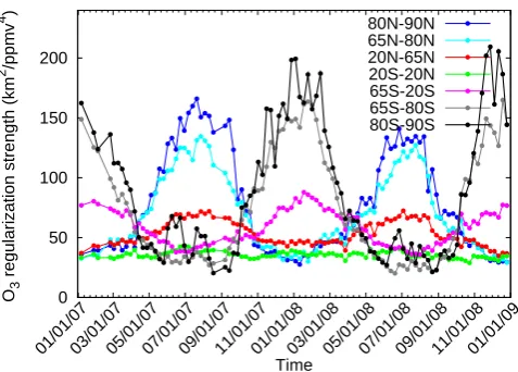
Fig. 1. Time evolution of the regularization strength used in ozone retrieval from January 2007 to December 2008 for the different latitude bands indicated in the plot’s key. Points represent weekly means.
where Scis the covariance matrix of the profile retrieved with
the regularizing Levenberg–Marquardt method (Eq. 7). As shown in Ceccherini (2005) and in Ceccherini et al. (2007a), this regularization parameter provides a significant but rather weak regularization. The existence of an analyt-ical expression makes the error consistency method partic-ularly suitable for implementation in operational retrievals, where the regularization is applied, without direct user su-pervision, to large sets of profiles with variable noise errors. Figure 1 represents the time evolution of the regularization strength for the ozone retrieval from January 2007 to De-cember 2008 for different latitude bands. The regularization strength presents significant latitudinal and seasonal behav-ior, that, according to Eq. (11), is anti-correlated with the retrieval error of the profile obtained with the regularizing Levenberg–Marquardt method.
The possibility of adapting the regularization strength to each observation according to its random error makes the bias introduced by the regularization always comparable with the random error. Furthermore, by ensuring that the relative weight of the measurements and the constraint in the cost function to be minimized is maintained approximately con-stant, the same relative regularization is applied to the pro-file even when the information content of the measurements changes significantly, with a consequent small variation of the vertical resolution (see Sect. 4.2).
with error consistency method) makes the retrieval more in-stable and the convergence slower.
After the a posteriori regularization the covariance and av-eraging kernel matrices, computed in Eqs. (7) and (8), are updated according to
S=
S−c1+λR
−1
S−c1S−c1+λR
−1
, (12)
A=S−c1+λR
−1
S−c1Ac. (13)
Since the strength of the regularization is driven by a sin-gle scalar parameterλindependent of altitude, the error con-sistency method is not suitable to regularize the water va-por profile for which the VMR and its absolute retrieval er-ror change by two orders of magnitude across the MIPAS retrieval range (6–70 km). An attempt was made to fix this problem by applying the regularization to the logarithm of the water VMR profile, which is equivalent to considering the relative error instead of the absolute one. However, this ap-proach fails when, because of the retrieval errors, a negative value of the water vapor VMR is retrieved. The constraining of the negative retrieved values to 10−10 parts per million
per volume (ppmv), as described in Sect. 3.6.1, did not help, because for this small value the approximation of the linear error propagation from the profile to the logarithm of the pro-file fails. In ML2PP V6 this problem with water vapor VMR regularization is temporarily avoided by disabling the a pos-teriori regularization in water vapor retrievals. In future ESA processor releases this problem will be tackled with a more sophisticated, self-adapting and altitude-dependent regular-ization scheme first proposed in Ridolfi and Sgheri (2009) and subsequently optimized for the near real time retrieval processors in Ridolfi and Sgheri (2011).
3.4 Upgrades in the auxiliary data
In addition to the changes in the algorithm, the analysis of the OR measurements required also new auxiliary data. The main change was made in the MW database, i.e., the database of the spectral intervals selected for the retrieval containing the best information on the target species and being less af-fected by systematic errors. The MW selection is based on the minimization of the total error, including both random and systematic errors (see Sect. 4.1). The change of the spec-tral resolution modifies the contribution of each of these er-rors and leads to a different optimized selection of MWs in the two phases of the mission. Furthermore, the MWs for the analysis of the OR measurements were selected using some modified estimation of these errors, according to the improved knowledge on some MIPAS instrument errors as described in Sect. 4.1.
Tables 3, 4 and 5 list the MWs selected for each species for the analysis of FR and OR measurements. The MWs used for the analysis of the FR measurements are the same as de-scribed in Raspollini et al. (2006). The spectral intervals an-alyzed in the OR measurements are 3–4 times, depending on
the different species, wider than those of the old operation mode, even if, because of the reduced spectral resolution, the number of measured spectral points is only 1.2–1.6 times greater. Some points of these MWs are masked (i.e., are not used in the retrieval), and the masks are different at different altitudes. In general the two sets of MWs have only a small number of spectral points in common.
The use of two separate sets of MWs, further than the change in the measurement scenario, represents a disconti-nuity between the two phases of the mission. The impact of this discontinuity on the retrieval performances is inves-tigated in terms of random and systematic error and spatial resolution in the subsequent sections, while the possible pres-ence of bias between the two phases of the mission due to the different systematic errors affecting the two sets of MWs and to the different measurement scenario will be investigated in a subsequent companion paper (Raspollini et al., 2013).
Further changes in the auxiliary data involve the MI-PAS dedicated spectroscopic database. ML2PP V6 uses V3.2 of the spectroscopic database. With respect to V3.1 de-scribed in Raspollini et al. (2006), V3.2 includes updates in NH3, OCS, NO, H2O2, HNO3, as well as updated
pres-sure broadening (and its temperature dependence) of H2O at
948.26288 cm−1.
The climatological profile dataset used (IG2 V4.1) is de-scribed in Remedios et al. (2007).
3.5 New products
Starting with ML2PP V6, four additional target species, namely, CFC-11, ClONO2, N2O5 and CFC-12, have been
operationally processed. These species are retrieved sequen-tially in this order after the retrieval of the original target species. With the addition of these new target species not only more variables of the atmospheric chemistry are de-termined providing a more comprehensive overview of the overall atmospheric composition, but also a better under-standing of the observed spectrum is attained. Indeed, the use of the retrieved profiles of these species, instead of the IG2, as assumed profiles in the retrieval of the other target species, reduces the errors due to the mutual interference of the species.
0 10 20 30 40 50 60 70 80
0 0.02 0.04 0.06 0.08 0.1 0.12 0.14 0.16
Altitude (km)
Ozone absolute noise error (ppmv) Latitude band: 65S-90S
DJF MAM JJA SON
0 10 20 30 40 50 60 70 80
0 5 10 15 20 25 30
Altitude (km)
Ozone percent noise error (%) Latitude band: 65S-90S
DJF MAM JJA SON
Fig. 2. Absolute (left plot) and percent (right plot) noise error of O3profile averaged on all profiles of the 65–90◦S latitude band in the four seasons of year 2008 (December 2007, January and February 2008 (DJF); March, April and May 2008 (MAM); June, July and August 2008 (JJA); September, October and November 2008 (SON)).
Table 3. Spectral intervals selected for the retrieval of pressure and temperature, H2O, O3and HNO3in the two phases of the mission.
FR OR
Spectral interval [cm−1] Altitude range [km] Spectral interval [cm−1] Altitude range [km] pT
685.7–685.825 33–47 703.375–703.875 21–37
686.4–689.4 30–68 719.0625–720.625 27–66
694.8–695.1 27–36 740.9375–743.9375 15–70
700.475–701.1 21–30 791.625–792.25 9–21
728.3–729.125 15–27 937.5–940.5 6–23
741.975–742.25 15–24 942.31–944.62 6–27
791.375–792.875 6–33
H2O
807.85–808.45 9–18 953.6875–956.6875 6–40
946.65–947.7 6–18 1223.75–1226.25 7.5–18
1645.525–1646.2 27–60 1387.5625–1390.5 12–70
1650.025–1653.025 15–68 1391.75–1394.75 12–54
1649.875–1652.875 15–66
O3
763.375–766.375 6–68 729.25–732.25 15–42
1039.375–1040.325 52–68 756.625–759.625 9–36
1122.8–1125.8 6–68 1043–1046 27–68
1117–1120 6–42
1123.5625–1126.5625 9–68
HNO3
876.375–879.375 6–42 836.875–839.875 6–42
885.1–888.1 6–42 859.5625–862.5625 9–42
877.0–880.0 6–42
893.625–896.625 6–42
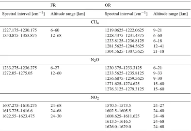
Table 4. Spectral intervals selected for the retrieval of CH4, N2O and NO2in the two phases of the mission.
FR OR
Spectral interval [cm−1] Altitude range [km] Spectral interval [cm−1] Altitude range [km] CH4
1227.175–1230.175 6–60 1219.0625–1222.0625 9–21
1350.875–1353.875 12–68 1228.4375–1231.4375 6–60
1233.8125–1236.8125 6–18 1281.5625–1284.5625 12–41 1304.5625–1307.5625 21–18
N2O
1233.275–1236.275 6–27 1230.375–1233.3125 6–21
1272.05–1275.05 12–60 1233.5625–1235.8125 9–33
1256.6875–1259.5625 9–30 1271.625–1274.625 15–60 1276.3125–1279.3125 15–60
NO2
1607.275–1610.275 24–68 1570.5–1573.5 24–27
1613.725–1616.6 24–68 1602.5–1605.5 24–60
1622.55–1623.475 24–30 1608.625–1611.625 24–48
1613.5–1616.5 24–68
1626.0–1629.0 24–68
is important in order to verify the decrease of CFC-11 and CFC-12 in the atmosphere due to the Montreal and succes-sive protocols (Kellmann et al., 2012). Concerning ClONO2
and N2O5molecules, they are important reservoir species for
nitrogen and chlorine in the stratosphere and play, therefore, an important role in the stratospheric ozone chemistry.
For some of the new species (especially N2O5) the
ob-served features are characterized by broad unresolved bands that are strongly correlated with the fitted atmospheric con-tinuum. Furthermore, the MWs that are used for the retrieval are located in a small spectral region, where the continuum can be assumed approximately constant. In this case, the ap-proach originally used of retrieving a continuum profile for each microwindow has been changed with the possibility of fitting, for selectable species, a single continuum profile com-mon for all the MWs, as also described in Mengistu Tsidu et al. (2004). This new approach is used for the retrieval of N2O5.
3.6 Other minor changes and caveats
For completeness in the following subsections we describe another minor change implemented in ML2PP V6 and a caveat.
3.6.1 Negative VMRs
In the previous versions of the ESA Level 2 proces-sor the VMR profiles were constrained to be greater than 10−10ppmv after each iteration for all species. This
constraint was introduced in order to avoid possible overflow errors in the radiative transfer calculation. However, when the random errors are comparable with the retrieved values of VMR it prevents the occurrence of negative values in the retrieval. This operation is physically justified but it may in-troduce a positive bias in the statistical distribution of the results. Biases emerged during the comparison of MIPAS FR measurements with correlative measurements, for example for CH4and N2O at high altitudes: from the comparison of
a sample of 131 coincident profiles of CH4in the 70–80◦N
latitude band of MIPAS and ACE–FTS (Atmospheric Chem-istry Experiment–Fourier Transform Spectrometer) measure-ments a positive bias (100·(MIPAS-ACE)/MIPAS) up to 80 %±8 % was estimated above 60 km for MIPAS (De Maz-ière et al., 2008). A similar positive bias is found in MIPAS ESA N2O profiles with respect to ACE–FTS (Strong et al.,
2008). A method for estimating the bias due to the positive constraint of the profiles is proposed in Funke et al. (2008).
In order to avoid the positive bias in the statistical dis-tribution of the results without reducing the robustness of the code, in ML2PP V6 the constraint to the VMR to be not smaller than 10−10ppmv has been maintained during the iterations but it is now removed at the last iteration. Test comparisons between ML2PP V6 and the previous version of the ESA processor indicate that the elimination of this constraint is successful in reducing the mean value of CH4
above 60 km and of N2O above 50 km of an amount
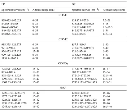
Table 5. Spectral intervals selected for the retrieval of CFC-11, CFC-12, N2O5and ClONO2in the two phases of the mission.
FR OR
Spectral interval [cm−1] Altitude range [km] Spectral interval [cm−1] Altitude range [km] CFC-11
839.625–842.625 6–33 824.875–827.0 7.5–21
842.65–845.65 6–33 835.0625–838.0625 6–18
846.45–849.45 9–33 839.875–842.875 7.5–16.5
849.475–852.475 6–33 842.9375–845.9375 6–34
853.075–856.075 6–33 849.5–852.5 13.5–34
CFC-12
918.375–921.375 6–39 857.5–860.5 6–40
921.4–924.4 6–39 917.9375–920.9375 6–40
924.425–927.425 12–39 921.0–924.0 6–40
929.125–932.125 6–39 933.625–936.625 6–37
1159.7–1162.7 6–39 937.0625–940.0625 12–40
ClONO2
778.525–781.525 18–42 777.4375–780.4375 18–37
805.4–808.4 18–39 807.375–810.375 15–34
808.425–811.425 15–36 1724.0–1727.00 13.5–40
1290.625–1293.625 15–42 1736.6875–1739.6875 13.5–43
1303.35–1306.35 15–42 1743.8125–1746.1875 13.5–31
N2O5
1220.0750–1223.075 15–42 1220.0–1223.0 15–46
1272.05–1275.05 15–42 1225.25–1228.25 15–46
1225.75–1228.75 15–42 1230.3125–1233.3125 15–40
1238.8250–1241.8250 15–42 1237.4375–1240.4375 18–46
1243.45–1246.45 15–42 1244.5625–1247.5625 16.5–46
The need to allow for negative values of the VMRs was identified also for other codes and other species (von Clar-mann et al., 2006).
3.6.2 Altitude bias
The MIPAS ESA Level 2 processor retrieves the pressure at the tangent levels and the temperature corresponding to this pressure. The spacing between two consecutive tangent al-titudes is determined from these quantities using the hydro-static equilibrium law constrained by the engineering infor-mation on the distance between two contiguous tangent al-titudes. The location of the altitude grid is determined using the lowest tangent altitude, assumed to be equal to the corre-sponding engineering value, as a reference point. In this way the tangent altitudes retrieved by the Level 2 processor are af-fected by a constant bias equal to the error of the engineering measurement at the lowest altitude, which may reach peak values as large as 1.5 km.
No correction of this bias is made in ML2PP V6, but the potential bias in the lowest retrieved tangent altitude has been estimated with a method that takes into account the height and pressure relation provided by the ECMWF atmospheric
model high resolution 10 day forecast data (ECMWF, 2009). By minimizing the function given by the sum of the square differences between each of three selected retrieved tangent altitudes (that are function of the lowest engineering tangent altitude) and the corresponding ECMWF value determined by interpolating the ECMWF altitude–pressure grid at the MIPAS pressure levels, the found correction applied to the lowest retrieved tangent altitude (computed on four days of measurements in the four seasons) has a standard deviation of 310 m.
4 Characterization of the Level 2 products in the two phases of the mission
In this section the quality of the products obtained by ML2PP V6 in the two phases of the mission is compared in terms of precision, accuracy and spatial resolution (both vertical and horizontal). It has to be highlighted that, even if the a poste-riori regularization is not necessary in the analysis of the FR measurements, it was decided to use it in order to have more consistent products on the whole MIPAS mission, also con-sidering that the a posteriori regularization does not change the convergence point and is completely reversible.
4.1 Accuracy and precision
The accuracy of the retrieved profiles is described in terms of the noise error and of the forward model errors.
The noise error is the mapping of the measurement noise in the retrieved profile and its covariance matrix S is computed using Eq. (12). The covariance matrix of the un-regularized retrieval Sc that appears in Eq. (12) is given by Eq. (7).
The covariance matrix of the observations Sy that appears
in Eq. (7) is calculated using the radiometric measurement noise (expressed in terms of noise equivalent spectral radi-ance, NESR) provided by the Level 1 processor, and takes into account the correlation between spectral points due to the apodization process (Raspollini et al., 2006; Ceccherini et al., 2007b). The noise error depends on the sensitivity of the measurements to the target parameters, in turn driven by the temperature profile. Given the large seasonal variability of the temperature profile, especially at latitudes far from the tropics, a large seasonal variability is also observed in the noise error. An example is shown for ozone in Fig. 2, where both the absolute (left plot) and relative (right plot) noise er-ror profiles, averaged in the latitude band 65–90◦S, are re-ported for the four seasons of 2008. The largest absolute er-rors are in general observed in the austral winter where the temperatures are coldest. A large relative error is present in the austral spring at the altitudes where ozone depletion oc-curs, but this is an effect of the significant decrease of ozone rather than a large change in the error.
The forward model errors are given by the propagation in the retrieved profiles of the uncertainties present in the in-strument and in the atmospheric model parameters, as well as of the approximations in the forward model itself (Dudhia et al., 2002). All these errorsi can be represented as a set of independent error vectorsδyi in the measurement space,
which are then mapped into corresponding retrieval errors
δxi asδxi=Tδyi, where T is the gain matrix (Eq. 6).
The uncertainties in the instrument and the atmospheric model parameters that have been used to estimate the sys-tematic errors of the retrieved profile are the same as used for the FR measurements and have already been reported in Raspollini et al. (2006). The only changes with respect to these values involve the uncertainty in the width of the
0 10 20 30 40 50 60 70 80
0 5 10 15 20
Altitude (km)
O3 random error (%) Noise FR Noise OR pT error FR pT error OR Random FR Random OR
Fig. 3. Contribution of noise error and pressure and temperature propagation error to the random error of O3for FR measurements (red curves) and OR measurements (green curves). All errors are in percentage.
apodized instrument line shape, where a value of 0.2 % in-stead of 2 % has been assumed for the data, and the radiance calibration errors in MIPAS bands C and D (see Table 1), for which the estimated error was changed from 2 to 1 %, based on a more accurate estimate of the errors made in the instru-ment line shape model and in the calibration.
Among the forward model errors, some are random, like the propagation of temperature and pressure noise errors on the VMR profiles (pT propagation error, Raspollini and Ridolfi, 2000), and some are systematic, such as the spectro-scopic errors. Others have a value and a variability that may depend on either the time or spatial scale of the profiles that are considered for the statistical analysis.
Here we estimate the single scan random error, for VMR retrievals, by quadratically summing the average single scan noise error and the average single scan error in VMR profiles due to the pT propagation error. The latter is computed by averaging, for a selected set of orbits, the diagonal elements of the covariance matrix of the pT propagation error relative to each VMR retrieval that is contained in the ESA Level 2 output files.
The contribution to the random error coming from the pT propagation error profile is generally not negligible with re-spect to the noise error. Figure 3 provides an example for O3of the different contributions to the random error for both
0 10 20 30 40 50 60 70
0 10 20 30 40 50
Altitude (km)
O3 error (%)
FR measurements rand sum
rand day rand equ rand ngt rand win rand glw syst sum syst day syst equ syst ngt syst win syst glw
0 10 20 30 40 50 60 70
0 10 20 30 40 50
Altitude (km)
O3 error (%)
OR measurements rand sum
rand day rand equ rand ngt rand win rand glw syst sum syst day syst equ syst ngt syst win syst glw
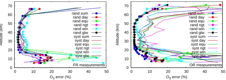
Fig. 4. Percent single scan random and systematic errors of O3profiles retrieved from FR (left plot) and OR (right plot) measurements. Both the average random error profiles and the estimated systematic error profiles are provided for the following five reference atmospheres: midlatitude daytime (day), midlatitude nighttime (ngt), polar summer daytime (sum), polar winter nighttime (win) and equatorial daytime atmospheres (equ) (Remedios et al., 2007). Random errors for the global atmosphere (glw) are obtained by averaging the random error profiles of a year of measurements, systematic errors for the global atmosphere are obtained by a composite of results for the five reference atmospheres, with twice the weight given to results from the polar winter case.
The systematic error contribution to the total error budget of the retrieved profiles has been computed as the square root of the quadratic sum of all forward model errors, except for pT propagation error.
Figure 4 shows the percent random and systematic single scan error profiles of the O3VMR, computed taking into
ac-count the contributions described above, for both FR (left plot) and OR (right plot) measurements. Corresponding fig-ures for pressure and temperature, as well as for the VMR of the other species, are reported in the Supplement to the online publication. The random error profiles, obtained by averaging the noise error on either one season or one year of measurements and including the contribution of the pT error propagation error, are shown for five reference atmospheres, i.e., midlatitude daytime (day), midlatitude nighttime (ngt), polar summer daytime (sum), polar winter nighttime (win), equatorial daytime (equ). The estimate of the systematic er-ror profiles is shown for the same reference atmospheres, which are also used for the MW selection (Remedios et al., 2007). Random errors for the global atmosphere (glw) are obtained by averaging the random error profiles of a year of measurements, systematic errors for the global atmosphere are obtained by a composite of results for the five reference atmospheres, with twice the weight given to results from the polar winter case, to ensure that this atmosphere, which is significantly different from the other four, is properly represented. The random error profiles change significantly for different atmospheric conditions, the polar winter atmo-sphere being characterized by the largest errors. The increase of the random error in polar winter conditions is particularly evident for CH4 (see Fig. 5), since it reaches 40 % for FR
measurements and 15 % for OR measurements around 30 km in South Pole winter conditions, while for the other latitudes and other conditions the random error does not exceed 10 % below 55 km. A similar increase in the random error in polar
winter conditions is visible also for other species, especially H2O, N2O, NO2and CFC-12 (not shown here, but reported
in the supplementary material to the online publication). Also the systematic errors show a dependence on the at-mospheric conditions.
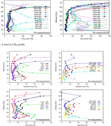
Figures 6 and 7 show, for FR and OR measurements re-spectively, the global yearly mean of the percent single scan random error profile for all analyzed species (top panels) and the corresponding single scan systematic error profile of the global atmosphere (bottom panels). The random error varies between 5 and 20 %, apart, for some species, near the bound-aries of the corresponding retrieval range. Similar random errors are obtained for all species in the two phases of the mission, thanks to the selection of a larger number of spec-tral points in the retrievals from OR measurements.
Also the systematic errors vary between 5 and 20 %, al-though for some species larger errors are obtained near the boundaries of the retrieval range. The systematic errors of FR and OR measurements are on the whole comparable, even though slightly larger errors are usually obtained for OR measurements.
We should also mention that, because we now apply a reg-ularization, the random errors of the FR measurements re-ported here are smaller than those obtained in the previous processing (see Raspollini et al., 2006). Accordingly, the ver-tical resolution of FR measurements is here degraded.
4.2 Vertical resolution
0 10 20 30 40 50 60 70
0 10 20 30 40 50
Altitude (km)
CH4 error (%)
FR measurements rand sum
rand day rand equ rand ngt rand win rand glw syst sum syst day syst equ syst ngt syst win syst glw
0 10 20 30 40 50 60 70
0 10 20 30 40 50
Altitude (km)
CH4 error (%)
OR measurements rand sum
rand day rand equ rand ngt rand win rand glw syst sum syst day syst equ syst ngt syst win syst glw
Fig. 5. Same as Fig. 4, but for CH4profile.
0 10 20 30 40 50 60 70
0 10 20 30 40 50
Altitude (km)
Random error (%)
FR measurements H2O
O3
CH4
N2O
N2O5
0 10 20 30 40 50 60 70
0 10 20 30 40 50
Altitude (km)
Random error (%)
FR measurements NO2 day
NO2 night
HNO3
CFC-11 CFC-12 ClONO2
0 10 20 30 40 50 60 70
0 10 20 30 40 50
Altitude [km]
Syst error [%]
FR measurements FR measurements
H2O
O3
CH4
N2O
N2O5
0 10 20 30 40 50 60 70
0 10 20 30 40 50
Altitude [km]
Syst error [%]
FR measurements FR measurements
NO2 day
NO2 night
HNO3
CFC-11 CFC-12 ClONO2
Fig. 6. Top panels: percent yearly mean of single scan random error profiles retrieved from FR measurements for the species indicated in the plots’ keys. Bottom panels: corresponding percent single scan systematic error profiles relative to the global atmosphere.
kernel matrix for two representative scans from FR measure-ments and OR measuremeasure-ments respectively. In the figures, the number of degrees of freedom for the considered scan are also indicated, given by the trace of the AK matrix. Typ-ical values for ozone are, in absence of clouds, 15 for FR measurements and 21.5 for OR measurements. Correspond-ing figures with the averagCorrespond-ing kernels of the other species are reported in the supplementary material to the online publica-tion. For altitudes lower than 30 km the peaks of FR averag-ing kernels are closer to 1 than those of OR ones, indicataverag-ing that for OR measurements a larger constraint is applied in this altitude range, as expected considering the different ill-conditioning of the retrievals. Nevertheless, the vertical res-olution of the profile is significantly better in OR measure-ments in this altitude range. Indeed, the vertical resolution,
further than depending on the constraint of the retrieval and on the IFOV size, is driven by the vertical retrieval grid which is taken equal, for most species, to the measurement grid and is, therefore, finer for OR measurement. The vertical reso-lution has been estimated as the ratio between the area sub-tended by the averaging kernel and its diagonal value. This quantity, which in the case of an undersampled distribution is also easily calculated, is an approximate estimation of the full width at half maximum (FWHM) of the averaging ker-nel rows, coinciding with it in case of a triangular form of the averaging kernel.
Figure 9 shows the vertical resolution profile (averaged on one orbit) and retrieval grid step for the O3profile for two
0 10 20 30 40 50 60 70
0 10 20 30 40 50
Altitude (km)
Random error (%)
OR measurements H2O
O3 CH4 N2O N2O5
0 10 20 30 40 50 60 70
0 10 20 30 40 50
Altitude (km)
Random error (%)
OR measurements NO2 day NO2 night HNO3 CFC-11 CFC-12 ClONO2
0 10 20 30 40 50 60 70
0 10 20 30 40 50
Altitude [km]
Syst error [%]
OR measurements OR measurements
H2O O3 CH4 N2O N2O5
0 10 20 30 40 50 60 70
0 10 20 30 40 50
Altitude [km]
Syst error [%]
OR measurements OR measurements
NO2 day NO2 night HNO3 CFC-11 CFC-12 ClONO2
Fig. 7. Top panels: percent yearly mean of single scan random error profiles retrieved from OR measurements for the species indicated in the plots’ keys. Bottom panels: corresponding percent single scan systematic error profiles relative to the global atmosphere.
the IFOV of approximately 3 km measured at tangent alti-tude point. In the OR measurements the use of a finer mea-surement grid step allows one to obtain an improved vertical resolution, which in the troposphere and lower stratosphere is often smaller than the IFOV of the instrument. Apart from the change in the vertical resolution due to the change in the measurement scenario, a very small variation of the verti-cal resolution is found also when a large seasonal variability is observed in the noise error (see Fig. 2). Figure 10 shows the ozone vertical resolution profile, averaged in the latitude band 65–90◦S, for the four seasons of 2008. The small vari-ation of the vertical resolution for different seasons is a con-sequence of the self-adapting regularization scheme that is used in the retrieval scheme (see Sect. 3.3).
The same considerations are valid for the profiles of the other species. Figures 11 and 12 show the vertical resolution profiles of the various species respectively for FR and OR measurements. For FR measurements the vertical resolution of all species is between 3 and 5 km in the altitude range 10– 40 km, and significantly larger above. For OR measurements the vertical resolution varies between 1.5 and 4 km in the alti-tude range 10–40 km for all species except CH4, N2O,
CFC-12 and CFC-11. For these four species similar performances are obtained in the two phases of the mission because the re-trieval of OR measurements is performed on a grid coarser than the measurement grid below 20 km, and hence the re-trieval grids are comparable in the two phases of the mission. In particular, the VMR was retrieved on every two points of the measurement grid for CH4in the altitude range 6–29 km,
for N2O in the altitude range 6–21 km, for CFC-11 in the
altitude range 6–18 km, for CFC-12 in the altitude range 6– 18 km and also for NO2in the altitude range 46–71 km.
The water vapor profile is characterized in the two phases of the mission by the best vertical resolution of all the other species, because no regularization is applied (see Sect. 3.3).
4.3 Horizontal resolution
The operational retrieval assumes local horizontal homo-geneity of the atmosphere, i.e., the vertical profiles are re-trieved assuming, at each limb scan, the atmosphere as made of homogeneous spherical shells (Raspollini et al., 2006; Ridolfi et al., 2000).
0 10 20 30 40 50 60 70
-0.2 0 0.2 0.4 0.6 0.8 1 O3 AK
DoF=15 FR measurements
0 10 20 30 40 50 60 70
-0.2 0 0.2 0.4 0.6 0.8 1 O3 AK
DoF=21.5 OR measurements
Fig. 8. O3averaging kernels for two representative scans of FR (left plot) and OR (right plot) measurements.
0 10 20 30 40 50 60 70 80
1 2 3 4 5 6 7 8 9 10
Altitude (km)
O3 vertical resolution and vertical step (km) OR vert. res.
OR step FR vert. res. FR step
Fig. 9. Vertical resolution profile and vertical retrieval steps for ozone profiles retrieved from FR measurements (green curves) and OR measurements (red curves), as indicated in the plot’s key.
A set of horizontal averaging kernels (HAKs), character-izing the horizontal smoothing of MIPAS measurements, has been computed as described in von Clarmann et al. (2009). This set includes HAKs for the MIPAS IG2 atmospheres (Version 4.1, Remedios et al., 2007), i.e., six latitude bands and four seasons for each year and for both FR and OR surements. The HAKs were calculated assuming the surement characteristics corresponding to the nominal mea-surement modes of both the FR and the OR scenarios (see Table 2).
For all the considered cases, the HAKs have a single max-imum, therefore it is meaningful to quantify their horizontal spread with the FWHM. We compute this quantity using the same method used for the estimation of the vertical resolu-tion (see Sect. 4.2).
The FWHM of the HAKs shows quite small variations as a function of both latitude and season, therefore here we show only the FWHM relating to a single month (July) and the average over the six latitude bands. Figures 13 (for FR) and 14 (for OR) show the FWHM of HAKs as a function of
0 10 20 30 40 50 60 70 80
2 3 4 5 6 7
Altitude (km)
Ozone vertical resolution (km) Latitude band: 65S-90S
DJF MAM JJA SON
Fig. 10. Ozone vertical resolution profile averaged on all profiles of the 65–90◦S latitude band in the four seasons of 2008 (DJF, MAM, JJA and SON 2008).
altitude. Each plot contains lines related to temperature and to the VMR of six MIPAS species, as indicated in the plot’s key.
In general, below about 40 km the FWHM of the FR HAKs is between 200 and 300 km for all MIPAS products; and those corresponding to OR are slightly smaller. Above 40 km, the FR HAKs is between 300 and 600 km, while those of OR are significantly better, still below 300 km except at the uppermost altitude.
Since the horizontal sampling step of MIPAS limb scans is about 510 km for FR measurements and about 410 km for OR measurements (see Table 2), in both cases the atmosphere turns out to be horizontally undersampled at most altitudes. Because of this undersampling, the horizontal resolution of MIPAS measurements in the nominal mode is better quanti-fied by the horizontal sampling (see Table 2) rather than by the FWHM of the HAKs.
0 10 20 30 40 50 60 70 80
1 2 3 4 5 6 7 8 9 10
Altitude (km)
Vertical resolution (km)
FR measurements T H2O O3
HNO3 CH4 N2O NO2
CFC-11 CFC-12 N2O5 ClONO2
Fig. 11. Vertical resolution profile ofT, H2O, O3, HNO3, CH4, N2O, NO2, CFC-12, CFC-11, ClONO2and N2O5retrieved from FR measurements.
0 10 20 30 40 50 60 70 80
1 2 3 4 5 6 7 8 9 10
Altitude (km)
Vertical resolution (km)
OR measurements T H2O O3 HNO3 CH4
N2O NO2 CFC-11 CFC-12 N2O5
ClONO2
Fig. 12. Vertical resolution profile ofT, H2O, O3, HNO3, CH4, N2O, NO2, CFC-12, CFC-11, ClONO2and N2O5retrieved from OR measurements.
geolocation of the tangent point and the point where most of the information comes from. While the retrieved profiles are assumed as geolocated at the tangent points of the limb scan from which they are retrieved, most of the information contributing to the retrieved values comes from air masses shifted towards the satellite with respect to the tangent points. This shift is positively correlated to the opacity of the atmo-sphere in the spectral region used for the retrieval, and hence it is important in case of large opacity of the MWs used in the retrieval and in presence of significant horizontal variability of the atmosphere. In these conditions the shift may reach, for temperature, the value of 150–200 km. Further details on this shift can be found in von Clarmann et al. (2009a), Carlotti and Magnani (2009), and Carlotti et al. (2013).
0 10 20 30 40 50 60 70
0 100 200 300 400 500 600
Altitude (km)
FWHM of Horizontal AKs (km) FR, July 2002
T H2O O3 HNO3 CH4
N2O
NO2
Fig. 13. FWHM of FR horizontal averaging kernels relating to tem-perature, and the VMR of H2O, O3, HNO3, CH4, N2O, NO2. The assumed atmosphere is the one from IG2, July 2002.
0 10 20 30 40 50 60 70
0 100 200 300 400 500 600
Altitude (km)
FWHM of Horizontal AKs (km) OR, July 2006
T H2O O3 HNO3 CH4
N2O
NO2
Fig. 14. FWHM of OR horizontal averaging kernels relating to temperature, and the VMR of H2O, O3, HNO3, CH4, N2O, NO2. The assumed atmosphere is the one from IG2, July 2006.
5 Conclusions
The ESA processor has been specifically designed for op-erating in near real time, and hence for working automati-cally in different atmospheric conditions, aimed to use the minimum amount of a priori information that may introduce a bias in the profiles.
The algorithm, originally designed for the scenario of the FR measurements, required some modifications for the anal-ysis of the OR measurements, to fully exploit the dense verti-cal sampling of the OR measurements with a proper handling of the ill-conditioned problem coming from the use of a re-trieval grid finer than the IFOV of the instrument.
Looking for self-adapting constraints, the ill-conditioned problem of the OR measurements is handled with the regu-larizing Levenberg–Marquardt approach during the iterations and an a posteriori regularization with a self-adapting con-straint dependent on the random error of each profile. An accurate method specifically designed for the regularizing Levenberg–Marquardt approach is used for the computation of the diagnostic quantities (covariance and averaging ker-nels). The innovative solutions implemented in ESA proces-sor and discussed in the paper can be useful for the analysis of future limb-sounding missions.
An overview of the performance of the ESA processor ML2PP V6, used for the re-analysis of the entire MIPAS mission, is presented for all the operational species, i.e., H2O, O3, HNO3, CH4, N2O, NO2, CFC-11, CFC-12, N2O5,
ClONO2, further than temperature, and a comparison
be-tween the two phases has been carried out. The performed analysis shows that the random and systematic error perfor-mances, thanks to the redundant information on the target species present in MIPAS spectra and the consequent use of dedicated MWs in the two phases (larger spectral intervals being used for OR measurements), are generally compara-ble in the two phases. The single scan random error varies between 5 and 20 % for most species and most altitudes. For the weakest species, near the boundaries of the retrieval range, the percent random error may be significantly larger than these values. The systematic errors are generally larger than the random errors, especially for the OR measurements. The profiles from OR measurements are characterized by an improved horizontal sampling (about 510 km for FR mea-surements, about 410 km for OR measurements) and an im-proved vertical resolution (varying, in the altitude range 10– 40 km, between 3 and 5 km for FR measurements, between 1.5 and 4 km for OR measurements) for most species.
In general, for the species we have analyzed, the OR mea-surements provide higher quality products than FR measure-ments.
The random errors, as well as the systematic errors, are de-pendent on the latitude and season. On the contrary, thanks to the use of a self-adapting regularization schemes in the re-trieval algorithm, a small variation of the vertical resolution is obtained for different atmospheric conditions. The mini-mal use of external constraints, which are prone to introduce
biases in the solution, makes ESA processor products suit-able for the climatological studies.
The use of different MWs in the two phases and in general the change in the measurement scenario impose some caution when using the full ten year dataset to extract trends. This issue will be further investigated in a subsequent companion paper (Raspollini et al., 2013).
Supplementary material related to this article is available online at http://www.atmos-meas-tech.net/6/ 2419/2013/amt-6-2419-2013-supplement.pdf.
Acknowledgements. This work has been performed under the ESA
study “Support to MIPAS Level 2 product validation”, contract ESA-ESRIN no. 21719/08/I-OL. The authors are grateful to the Astrium team that developed the industrial prototype ML2PP using the ORM code as reference, to Thorsten Fehr and Rolf von Kulhmann for the coordination of the MIPAS Quality Working Group activities and to Michael Kiefer for the work done within the MIPAS Quality Working Group.
Edited by: A. Lambert
References
Bermejo-Pantaleón, D., Funke, B., López-Puertas, M., García-Comas, M., Stiller, G. P., von Clarmann, T., Linden, A., Grabowski, U., Höpfner, M., Kiefer, M., Glatthor, N., Kell-mann, S., and Lu, G.: Global observations of thermospheric tem-perature and nitric oxide from MIPAS spectra at 5.3 µm, J. Geo-phys. Res., 116, A10313, doi:10.1029/2011JA016752, 2011 Böckmann, C., Kammanee, A., and Braunss, S.: Logarithmic
con-vergence rate of Levenberg-Marquardt method with application to an inverse potential problem, J. Inverse and Ill-Pose. P., 19, 345–367, doi:10.1515/JIIP.2011.034, 2011.
Carlotti, M.: Global-fit approach to the analysis of limb-scanning atmospheric measurements, Appl. Optics, 27, 3250–3254, 1988. Carlotti, M. and Magnani, L.: Two-dimensional sensitivity analysis
of MIPAS observations, Opt. Expr., 17, 5340–5357, 2009. Carlotti, M., Brizzi, G., Papandrea, E., Prevedelli, M., Ridolfi, M.,
Dinelli, B. M., and Magnani, L.: GMTR: two-dimensional geofit multitarget retrieval model for Michelson Interferometer for Pas-sive Atmospheric Sounding/environmental satellite observations, Appl. Optics, 45, 716–727, 2006.
Carlotti, M., Arnone, E., Castelli, E., Dinelli, B. M., and Papan-drea, E.: Position error in profiles retrieved from MIPAS obser-vations with a 1-D algorithm, Atmos. Meas. Tech., 6, 419–429, doi:10.5194/amt-6-419-2013, 2013.
Ceccherini, S.: Analytical determination of the regularization pa-rameter in the retrieval of atmospheric vertical profiles, Optic. Lett., 30, 2554–2556, 2005.