A simulated annealing algorithm for unequal area dynamic facility layout problems with flexible bay structure Pages 307-330 Download PDF

(1)

International Journal of Industrial Engineering Computations 9 (2018) 307–330

Contents lists available at GrowingScience

International Journal of Industrial Engineering Computations

homepage: www.GrowingScience.com/ijiec

A simulated annealing algorithm for unequal area dynamic facility layout problems

with flexible bay structure

Irappa Basappa Hunagunda*, V. Madhusudanan Pillaib and U.N.Kempaiahc

a_{Department of Mechanical Engineering, Government Engineering College Ramanagar, Ramanagar- 562159, Karnataka, India} b_{Department of Mechanical Engineering, National Institute of Technology Calicut, Calicut- 673 601, Kerala, India}

c_{Department of Mechanical Engineering, University Visvesvarayya College of Engineering, Bangalore- 560001, Karnataka, India} C H R O N I C L E A B S T R A C T

Article history: Received July 18 2017 Received in Revised Format August 20 2017

Accepted August 26 2017 Available online August 27 2017

In this article, we propose Simulated Annealing (SA) heuristic to solve Unequal Area Dynamic Facility Layout Problem (FBS) with Flexible Bay Structure (DFLPs with FBS). The UA-DFLP with FBS is the problem of determining the facilities dimension and their location coordinates with flexible bays formation in the layout for various periods of the planning horizon. The UA-DFLP with FBS is more constrained than general UA-DFLP and it is an NP-complete problem. The proposed SA is tested with the available UA-DFLPs instances in the literature. The proposed SA heuristic has given new best solution or the same solution for FBS based problems as compared with the best-known reported in the UA-DFLPs with FBS literature. The proposed SA heuristic is also tested on standard UA-DFLPs used in non-FBS approaches. The SA heuristic solution is not significantly different from the best solution reported in the literature for non-FBS approaches. Equal area DFLP instances are also solved with the proposed SA and the results obtained are promising with the solutions reported in the literature. Hence the results obtained indicate that the proposed SA for UA-DFLP with FBS is effective and versatile for both equal and unequal area dynamic facility layout problems. The computational efficiency of the proposed SA heuristic is very much competitive as compared to other meta-heuristics computational timings reported in the literature.

Unequal area dynamic facility layout problems

Flexible bays Simulated annealing Adaptive strategy

1. Introduction

(2)

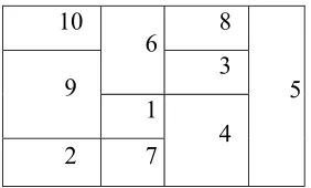
bays in the layout plan helps in the design of proper aisle structure on the shop floor, which in turn facilitates easy movement of material handling equipment on the shop floor. Hence, Konak et al. (2006) argued that the recent works on unequal area facility layout problems consider the Flexible Bay Structure (FBS) for the facility layout design. Tate and Smith (1995) published a key paper on FBS. In FBS, the plant floor is partitioned in one direction with bays of varying width and also each facility is assigned to a single bay. The bay width is flexible because the width of bay depends on the sum of the area of facilities within the bay. A sample of FBS representations for ten unequal area facilities is shown in Fig. 1. Further, Mazinani et al. (2013), for the first time, developed the Mixed Integer Linear Programming (MILP) model for UA-DFLPs with FBS and solved the model using GAMS software and Genetic Algorithm (GA).

Simulated Annealing (SA) algorithm is widely used in the literature to solve complex engineering problems. It is a global optimisation meta-heuristic. Unlike other meta-heuristics, SA is simple to implement, and it is sequential search algorithm. Hence it is computationally more efficient one. In this paper, SA algorithm is developed to solve the UA-DFLP with FBS and also the part handling factor is included in the Mazinani et al. (2013) MILP model of the UA-DFLP with FBS. The application of SA to UA-DFLP with FBS demonstrated the better performance compared to other meta-heuristic used in the literature.

The rest of the paper is organised as follows: Section 2 gives the review of literature and Section 3 discusses the MILP model of the UA-DFLP with FBS. Section 4 describes SA intuition, solution encoding, perturbation methods and SA flow chart. Section 5 gives numerical experiments, results and discussion. Section 6 presents the conclusions and scope for future work.

10

6 8

5

9 3

1

4 2 7

Fig. 1. Flexible bay structure representation of facilities in the layout 2.Literature Review

(3)

I. B. Hunagund et al.

Konak et al. (2006) reported that in continuous space, Montreuil (1990) was the first to develop Mixed Integer Problem (MIP) formulation for the Unequal Area Facility Layout Problems (UA-FLPs).UA-FLP is a NP-Complete problem (Drira et al., 2007). The complexity of the UA-FLP is due to a large number of binary variables in the MIP model. In case of Unequal Area Dynamic Facility Layout Problem (UA-DFLP), the introduction of periods makes the MIP model more complex. Hence, the optimal solutions for the UA-DFLP can be obtained only for small size problems. Therefore, researchers use different heuristics or meta-heuristics to solve UA-DFLPs. Montreuil (1990) model assumes the unlimited space for design and the model contains the non-linear area constraints. Lacksonen (1994, 1997) and Meller et al. (1998) approximated the non-linearity in the formulation with linear approximation constraints to make model simple. However, facilities area approximated with linear constraints are expected to have area errors. In this case, the facilities areas in the final solution are lesser than required. The assumption of no limit on available floor space in a MIP model makes the facilities clustering towards the centre of the plant. The drawback of facilities clustering towards the centre of the plant is overcome by fixing the floor size. In that case, the facilities are arranged either in Slicing Tree Structure (STS) or in Flexible Bay Structure (FBS). In STS, the plant floor is partitioned both in vertical and horizontal directions simultaneously (Scholz et al., 2009; Komarudin & Wong, 2010; Aiello et al., 2012). In FBS, the plant floor is partitioned either in vertical or horizontal direction, but not in both directions (Tate & Smith, 1995; Konak et al., 2006; Wong & Komarudin, 2010; Kulturel-Konak & Konak, 2011; Ulutas & Kulturel-Konak, 2012; Garcia-Hernandez et al., 2013; Garcia-Hernandez et al., 2015; Palomo-Romero et al., 2017). Konak et al. (2006) presented an MILP model for UA-FLP with FBS, and the authors converted the non-linear area constraints in the earlier MIP model into linear constraints. This formulation has the limitation on the size of problems that can be solved optimally. Hence, researchers use different meta-heuristics to solve Konak et al. (2006) model (Wong & Komarudin, 2010; Kulturel-Konak & Kulturel-Konak, 2011; Ulutas & Kulturel-Kulturel-Konak, 2012; Palomo-Romero et al., 2017). Further, few works considered the multi-objectives in the FBS based UA-FLPs (Garcia-Hernandez et al., 2013; Garcia-Hernandez et al., 2015). UA-FLP based on FBS is more constrained than STS based model due to the formation of bays in the FBS model. Hence, solution based on FBS is expected to have a poor Material Handling Cost (MHC) as compared to the solution based on STS. But, the bay structure in FBS helps to create proper aisles on the floor space. Thus, the difference in the MHC of the layout under FBS and practically implemented layout is less. Hence in the present study flexible bay structure (FBS) is considered for UA-FLPs.

(4)

at their starting locations of the period one. None of the above-mentioned works on UA-DFLP has considered the FBS in the layout solution.

Mazinani et al. (2013) for the first time developed the MILP model for UA-DFLPs with FBS and solved the model using GAMS software and GA. This model considers the shape constraint for the facilities instead of fixed dimension for facilities. In this formulation, area constraints are linear, and the facilities’ dimension is decision variables. The limitation in the solution methodology (GA) of the Mazinani et al. (2013) is that it can only be used for given maximum number of bays as input data. Further, Abedzadeh et al. (2013) presented the multi-objective formulation for UA-DFLP with FBS and authors used the parallel variable neighbourhood search and fuzzy concept as a solution method. Simulated Annealing (SA) is another simple heuristic used to solve combinatorial problems. Unlike other meta-heuristics, SA is simple to implement, and it is sequential search algorithm hence it is computationally more efficient one. Application of SA is made for solving equal area static and dynamic facility layout problems (Whim & Ward, 1987; Baykasoglu & Gindy, 2001; McKendall Jr et al., 2006; Pillai et al.,

2011). Tam (1992) used SA for general type UA-FLPs but not for UA-DFLP with FBS. Recently,

Kulturel-Konak and Konak (2015) used SA heuristic to solve unequal area cyclic facility layout problems, but it is not based on FBS. The research works (Kusiak & Heragu, 1987; Balakrishnan & Cheng, 1998; Singh & Sharma, 2006; Drira, et al., 2007; Moslemipour et al., 2012) give the detailed review of various types of facility layout problems and different heuristic and meta-heuristic approaches followed to solve the FLPs. To the best of our knowledge, no research work has observed in the literature, the application of SA algorithm to solve UA-DFLP with FBS.

An extensive literature review reveals that, FBS is one of the important layout representations that researchers focused for studying. In addition, the volatile market environment necessitates the consideration of UA-DFLPs. Since, UA-DFLP is the NP-Complete problem and therefore there is a need to develop better solution approaches to solve UA-DFLP with FBS. SA is a simple probabilistic search and computationally less intensive heuristic compared to other meta-heuristics. Hence, in this paper, the simulated annealing procedure is developed to solve UA-DFLP with FBS. The variation in the effort required to handle the product at various stages of production is also included in the UA-DFLP with FBS model of Mazinani et al. (2013) to compute actual flow matrices. Actual flow matrices are computed based on various periods’ product demand and effort required for transportation of products.

3.MILP model of UA-DFLP with FBS

In this section, Mazinani et al.’s (2013) MILP model for UA-DFLP with FBS is presented for reference. In this model, we consider the part handling factor as suggested by Chan et al. (2002) to calculate the realistic material flow between facilities. Even though the final product demand is unchanged, the best possible layout could be different if the part handling factor/effort data is inputted to the UA-DFLP with FBS model. Mazinani et al.’s (2013) MILP model with addition of part handling factor Eq. (30) is given below.

Inputs to the model:

 Number of periods in planning horizon.

 Number of facilities.

 Different period’s product flow between facilities.

 If material flow between facilities is not given then it is computed from number of products to be manufactured, the demand of products in various periods, operational sequence of products, and product-handling effort required at various operational stages.

 Area and maximum aspect ratio of each facility.

(5)

I. B. Hunagund et al. Notations:

Indexes;

k= 1, 2, ..., K, where K is the number of products

p= 1, 2, ..., P, where P is the number of periods

m, n= 1, 2, ..., N, where N is the number of facilities

r, s = 1, 2, ..., M, where M is the maximum number of bays

Input Parameters;

W Horizontal length of floor in x–axis direction

H Vertical length of floor in y–axis direction

p m

A _, Facility m area in period p of the planning horizon

p m,

 Facility m maximum aspect ratio in period p of the planning horizon



mp mp



p

m H A

S , ,

max

, min ,  Facility m maximum allowable side length in period p

p m

p m p

m

A S

, , min

,  _ Facility m minimum allowable side length in period p

p n m

f

_ _, Product flow volume from facility m to facility n in period p

p m n p n m p

mn

f

'

_,



_ _,



_ _, Product flow volume from facility m to facility n, and facility n to facility

m in period p

p mn

C

_, Cost of transporting unit product per unit distance from facility m to

facility n in period p

p n m k, ,



Part handling effort required for product k when moved from facility m to

p n m k

Z

_, __, Batch size of product k per movement when moved from facility m to

p k

D

_, Product k demand in period p

p m

F

_, Fixed rearrangement cost for shifting facility m at the beginning of period

p

p m

V

_, Variable rearrangement cost for shifting facility m at the beginning of

period p

(6)

Decision Variables;

p r

b_, Bay r horizontal width (length in x-axis direction) in period p

p mr

l _, Facility m height in bay r in period p

y p m

h , Facility m vertical height in y-axis direction in period p



xm,p,ym,p



Centre coordinates of the facility m in period p p n p m x p

mn x x

D ,  ,  , Distance between the centres of facilities m and n in x-axis direction in

period p

p n p m y p

mn y y

D ,  ,  , Distance between the centres of facilities m and n in y-axis direction in

period p

1 , ,

,  mp  mp

x p

m x x

P Amount of distance moved by facility m from period p-1to p in x-axis

direction

1 , ,

,  mp mp

y p

m y y

P Amount of distance moved by facility m from period p-1to p in y-axis

direction 1

. 

mr p If facility m is allocated to bay r in period p

0

 Otherwise

1

,p  r



If bay r is having facilities in period p

0

 Otherwise

1

,p



mn

Y

If facility m is above the facility n in the same bay in period p

0

 Otherwise

1

,p  m

Q If facility m is rearranged at the beginning of period p

0 Otherwise

Mathematical model:

, , , , , , , , ,

1 1 2 1 2 1

min P N N ' ( x y ) P N ( x y ) P N

mn p mn p mn p mn p m p m p m p m p m

p m n m p m p m

PHC C f D D V P P F Q

                   (1) subjected to; p m n m x x

Dmnx ,p  m,p n,p  ,  , (2)

p m n m x x

Dx _n_p _m_p p

mn,  ,  ,  ,  , (3)

p m n m y y

Dy _m_p _n_p

p

mn,  ,  ,  ,  , (4)

p m n m y y

Dy _n_p _m_p

p

mn,  ,  ,  ,  , (5)

1 ,

1 , ,

, x x  m p

Px _m_p _m_p p m (6) 1 , , 1 ,

, x  x m p

Pmxp mp mp (7)

1 ,

1 , ,

, y y  m p

Py _m_p _m_p p

(7)

I. B. Hunagund et al. 1 , , 1 ,

, y  y m p

Py _m_p _m_p

p m (9) p m I M r p

mr 1 ,

1 ,  



 (10) p r A I H b N m p m p mr p r , 1 1 , , , 



  (11)



I



mr p

W S b

S_m_p _r_p _mmax_p 1 _mr_,_p , ,

, , min

,      (12)

p r m I S W b b

x _m_p _mr_p

r s p r p s p

m 0.5 ( )(1 , ) , ,

min , , , , 



      (13) p r m I S W b b

x mp mrp

r s p r p s p

m 0.5 ( )(1 , ) , ,

min , , , , 



      (14) p m n m r I I A S A S A l A l p nr p mr p n p n p m p m p n p nr p m p

mr _max _, ₍₂ ₎ ₀ _, _, _,

, , , max , , max , , , , , _ _ _ _ _           (15) p m n m r I I A S A S A l A l p nr p mr p n p n p m p m p n p nr p m p

mr _max _, ₍₂ ₎ ₀ _, _, _,

, , , max , , max , , , , , _ _ _ _ _           (16) p r H l N m p r p mr , 1 , ,  







(17)



I



mr p

W I

S l I

S_m_p _mr_p _mr_p _mmax_p _mr_,_p 1 _mr_,_p , ,

, , , min

,      (18)

p m h l M r y p m p mr , 1 , ,  



 (19)



Y



m n m p

H h y

h

y y _mn_p

p n p n y p m p

m, 0.5 ,  , 0.5 ,  1 ,  ,  , (20)

p

m

n

m

Y

_mn_,_p



_nm_,_p



1



,



,

(21)

p

m

n

m

r

I

Y

_mn_,_p



_nm_,_p



_mr_,_p



_nr_,_p



1



,



,

(22)

p m h H y h y p m p m y p

m 0.5 ,

5 .

0 _,  _,   _,  (23)

1

,

1 ,

,



x





WQ



m

p



x

_m_p _m_p _m_p (24)

1

,

, 1

, 



x



WQ



m

p



x

_m_p _m_p _m_p (25)

1

,

1 ,

,



y





HQ



m

p



y

_m_p _m_p _m_p (26)

1

,

, 1

, 



y



HQ



m

p



y

_m_p _m_p _m_p (27)

1

,

1 ,

,



h





HQ



m

p



h

y _m_p p m y p m (28)

1

,

, , 1

, 



h



HQ



m

p



h

y _m_p p

m y

p

(8)

n m p Z

D

f K _k_m _n_p

k km np

p n m k p

n

m , , , ,

1 , ,

, ,

,   

 







(30)

p r n m P

P D D l b h y

x y

p m x

p m y

p mn x

p mn p mr p r y

p m p m p

m, , , , , , , , , , , , , , , , , 0  , , , (31)

 

Y

 

Q

m

n

r

p

I

_mr_,_p



0

,

1

,



_r_,_p



0

,

1

,

_mn_,_p



0

,

1

,

_m_,_p



{

0

,

1

}



,

(32)

In the above formulation, the objective function (1) consists of three terms, material handling costs, variable rearrangement costs and fixed rearrangement costs, respectively. Variable rearrangement costs and fixed rearrangement costs will be active only when there is a relocation of facilities takes place in subsequent periods to make trade off with the material handling costs of the first term. The objective function finds the facilities dimension and location coordinates while minimizing the planning horizon total cost.

The centre coordinates of facilities are defined by constraints (2-5). In these constraints, the absolute values expression x_m_,_px_n_,_p is linearized by mp np

x p

mn x x

D ,  ,  , and np mp

x p

mn x x

D ,  ,  , where , 0

x p mn

D

.Similarly, each facility shifting distance from one period to next period is defined by constraints (6-9). In these constraints also, the absolute values expression x_m_,_px_m_,_p_₁ is linearized by _,  m_,p m_,p₁

x p

m x x

P

and Pmx,p xm,p1xm,p wherePmx,p 0. The non-spreading of the facility to more than one bay is ensured by constraint (10). The width of each bay is computed using equation (11) based on the areas of the facilities assigned and the height of floor space. Constraint (12) ensures that width of each bay is within the maximum and minimum side length of facilities allocated in that bay. The facilities centre coordinates in x-axis direction are determined by constraints (13) and (14). Each facility is within the horizontal boundary (x-direction) of plant floor is ensured by constraints (11), (13) and (14). The facilities centre coordinates in y-axis direction are determined by constraints (15) to (22). These constraints also ensure that facilities do not overlap in the y-axis direction. Each facility is within the vertical boundary (y -direction) of plant floor is ensured by constraints (23). Constraints (24) to (29) ensure that the facility has the same value of length, width and center coordinates in any two sequential periods if facility is not relocated. The actual material flow volume between the facilities in the different periods of planning horizon are computed using equation (30), when the demand for the products with their part handling effort and the batch size are given. The non-negativity restriction on continuous decision variables is ensured by constraints (31) and constraint (32) puts the restriction on binary decision variables.

4.The simulated annealing algorithm for UA-DFLP with FBS

In this section, the working principle of SA, solution encoding, neighbourhood moves, SA parameters and SA flow chart are discussed. The simulated annealing algorithm was initially proposed by Kirkpatrik et al. (1983) for engineering optimization. SA is a global optimization heuristic. Many meta-heuristics like genetic algorithm, ants colony optimisation, particle swarm optimisation, artificial immune system, etc. are available in the literature for global optimization but all these are population-based parallel search algorithms. The SA works population-based on probabilistic methods that avoid being stuck at local minima. It is proven to be a simple sequential search algorithm but robust method for problems which are computationally more complex. Its optimization principle comes from the annealing process in metallurgy. The concept is based on the manner in which liquids freeze or metals recrystallize in the process of annealing.

In SA, the neighborhood solution A’ generated from a current solution A is not only accepted if A’ is better, but it may also be get accepted if A’ is worse than A. Worse solution is accepted with some acceptance probability. Boltzmann’s law is used to determine this acceptance probability, It is given as

P(accept)=exp (- Δ/(b × TS) ), where ‘b’ is Boltzmann’s constant and ‘TS’ is the temperature at each

(9)

initial and final temperatures respectively.Δ =z(A’)-z(A). The acceptance of new solution is done with the Metropolis criteria which is a function of temperature (TS) of the system and difference in cost (Δ).

That is, the lesser the increase in the ‘Δ’ value, more likely the neighbor solution is accepted, and the lower the value of ‘TS’, the less likely the neighbor solution is accepted.

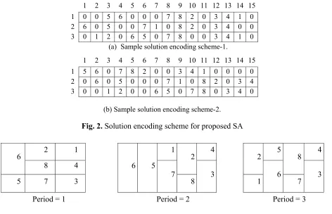
4.1 Solution encoding scheme

The UA-DFLP with FBS solution is encoded as a two dimensional matrix. The rows of the matrix represent the periods in planning horizon and elements of each row represent the facilities names and bay break points. The number of columns in the matrix is equal to the number facilities plus maximum number of bays in the layout. Hence, the matrix contains the complete information regarding period of planning horizon, an identity of facilities, facilities order and the bay break points of the layout. The numbering of bays in each period is from left to right and the order of facilities within the bays is from bottom to top. If the number of bays is not given, then the maximum number of bays in each period can be equal to the number of facilities. Hence the highest number of bay breakpoints in each row (period) can be (N-1), where N is the number of facilities. Then the number of columns in the matrix is taken as(2N-1). ‘0’ element after one or more facility in each row (i.e., in each period) represents bay break point. If the maximum number of bays (M) is a given data, then the number of columns in the matrix is

(N+M-1). The solution encoding scheme for 8-facilities with 3-period in planning horizon and

consideration of maximum number of bays in the layout equal to the given number facilities is shown in Fig. 2. Fig. 2 (a, b) show two sample solution encoded matrixes having the same layout configurations for eight facilities with three periods in the planning horizon. The layout configurations for these matrixes are shown in Fig. 3. The number of rows in the matrix = P = 3, and number of columns in the matrix =2N-1 =2×8-1 =15.

1 2 3 4 5 6 7 8 9 10 11 12 13 14 15

1 0 0 5 6 0 0 0 7 8 2 0 3 4 1 0

2 6 0 5 0 0 7 1 0 8 2 0 3 4 0 0

3 0 1 2 0 6 5 0 7 8 0 0 3 4 1 0

(a) Sample solution encoding scheme-1.

1 2 3 4 5 6 7 8 9 10 11 12 13 14 15

1 5 6 0 7 8 2 0 0 3 4 1 0 0 0 0

2 0 6 0 5 0 0 0 7 1 0 8 2 0 3 4

3 0 0 1 2 0 0 6 5 0 7 8 0 3 4 0

(b) Sample solution encoding scheme-2.

Fig. 2. Solution encoding scheme for proposed SA

6 2 1

6 5

1

2 4 2 5 8 4

8 4

7 3 6 3

5 7 3 8 1 7

Period = 1 Period = 2 Period = 3

(10)

4.2 Neighbourhood move

In the proposed study, the transition from one configuration to another is made by selecting the period (row) randomly and then applying the three operations namely, insert, swap and reversion on the randomly selected period. The three operations are used randomly with the equal probability of selecting each operation. That is, a random number r is generated between 0 and 1, if the r is between 0r0.33 insert operation is carried out and if the r is between 0.33r0.67swap operation is carried out and if the r is between 0.67r1reversion operation is carried out for neighbourhood configuration creation. After generating the neighbourhood solution using randomly selected operation, the algorithm checks the feasibility of solution; if the solution is infeasible then the randomly selected operation is repeated on the randomly selected period (row) until a feasible solution is obtained.

Insert operation

In this operation, two random numbers i and j between 1 and length of row (period) are generated. These random numbers indicate the positions of element in a randomly selected row (period). The insert operation removes the element in the position i of the row and then moves certain elements either leftward or rightward depending on values of i and j and then insert the removed element into the position j. If i

<j, the element in the position i is removed and the elements from position i+1 to j are moved one position leftward, then the removed element is inserted into position j. If i > j, the element in position i is removed and the elements from position j to (i-1) are moved one position rightward, then the removed element is inserted into position j. Insert operation can change the number of bays in the layout or it can change the number of facilities within bays for the randomly selected period, hence it is a versatile operator. For randomly selected period-1 (row-1), the insert operation on the encoded matrix-1of the Fig. 2(a) is illustrated in Fig. 4. In Fig. 4(a), the insert operation creates a neighbourhood solution without a change in the number of bays, but it changed the number of facilities within each bay. In Fig. 4(b), the insert operation merged the bays 2 & 3 and converted them into a single bay to form a neighbourhood solution. In Fig. 4(c), the insert operation created a new bay in the neighbourhood solution by splitting the bay 1 into two new bays.

Before insert operation After insert operation

1 2 3 4 5 6 7 8 9 1011 12 13 14 15 1 2 3 4 5 6 7 8 9 10 11 12 13 14 15

1 0 0 5 6 0 0 0 7 8 2 0 3 4 1 0 1 0 0 5 6 2 0 0 0 7 8 0 3 4 1 0 2 6 0 5 0 0 7 1 0 8 2 0 3 4 0 0 2 6 0 5 0 0 7 1 0 8 2 0 3 4 0 0 3 0 1 2 0 6 5 0 7 8 0 0 3 4 1 0 3 0 1 2 0 6 5 0 7 8 0 0 3 4 1 0

(a) Insert operation for random number p = 1, and i = 10 &j = 5.

1 2 3 4 5 6 7 8 9 101112 13 1415 1 2 3 4 5 6 7 8 9 10 11 12 13 14 15

1 0 0 5 6 0 0 0 7 8 2 0 3 4 1 0 1 0 0 5 6 0 0 0 7 8 2 3 4 1 0 0 2 6 0 5 0 0 7 1 0 8 2 0 3 4 0 0 2 6 0 5 0 0 7 1 0 8 2 0 3 4 0 0 3 0 1 2 0 6 5 0 7 8 0 0 3 4 1 0 3 0 1 2 0 6 5 0 7 8 0 0 3 4 1 0

(b)Insert operation for random number p = 1, and i = 11 &j = 15.

1 2 3 4 5 6 7 8 9 10 11 12 13 14 15 1 2 3 4 5 6 7 8 9 10 11 12 13 14 15

1 0 0 5 6 0 0 0 7 8 2 0 3 4 1 0 1 0 0 5 0 6 0 0 7 8 2 0 3 4 1 0 2 6 0 5 0 0 7 1 0 8 2 0 3 4 0 0 2 6 0 5 0 0 7 1 0 8 2 0 3 4 0 0 3 0 1 2 0 6 5 0 7 8 0 0 3 4 1 0 3 0 1 2 0 6 5 0 7 8 0 0 3 4 1 0

(c)Insert operation for random numbers p = 1, and i = 7 &j = 4.

(11)

I. B. Hunagund et al. Swap operation

In this operation the element in positions i and j of the randomly selected period are swapped. Application of swap operation is shown in Fig. 5 for randomly selected period-3. Note that if the element of positions

i and j are bay breaks ‘0’ then the swap operation does not generate different neighbourhood solution from the current solution; in that case the new i and j are generated until the elements in i and j positions are not bay breaks ‘0’.

Before reversion operation After reversion operation

1 2 3 4 5 6 7 8 9 10 11 12 13 14 15 1 2 3 4 5 6 7 8 9 10 11 12 13 14 15 1 0 0 5 6 0 0 0 7 8 2 0 3 4 1 0 1 0 0 5 6 0 0 0 7 8 2 0 3 4 1 0 2 6 0 5 0 0 7 1 0 8 2 0 3 4 0 0 2 6 0 5 0 0 7 1 0 8 2 0 3 4 0 0

3 0 1 2 0 6 5 0 7 8 0 0 3 4 1 0 3 0 7 2 0 6 5 0 1 8 0 0 3 4 1 0

Fig. 5. Swap operation illustration for random period-3 with random numbers i = 8 and j = 2

Reversion operation

This operation reverses all the elements located from the position i to the position j. In this configuration change, the reverse operation sequentially removes the elements from positions i to j in current solution and places these elements sequentially into positions j to i in reverse manner to create neighbourhood solution. Application of reversion operation is shown in Figure 6 for randomly selected period-2.

Before reversion operation After reversion operation

1 2 3 4 5 6 7 8 9 10 11 12 13 14 15 1 2 3 4 5 6 7 8 9 10 11 12 13 14 15 1 0 0 5 6 0 0 0 7 8 2 0 3 4 1 0 1 0 0 5 6 0 0 0 7 8 2 0 3 4 1 0

2 6 0 5 0 0 7 1 0 8 2 0 3 4 0 0 2 6 0 5 8 0 1 7 0 0 2 0 3 4 0 0 3 0 1 2 0 6 5 0 7 8 0 0 3 4 1 0 3 0 1 2 0 6 5 0 7 8 0 0 3 4 1 0

Fig. 6. Reversion operation illustration for random period-2 and random numbers i = 4 and j = 9

4.3 SA Parameters settings

 Solution perturbation: The three operations explained in Section 4.2 are used on the randomly selected period to move into the neighbourhood configuration from the current configuration. The operators are used randomly on the randomly selected period with the equal probability of selecting each operator.

 Starting temperature (Ts): The starting temperature must be hot enough to accept almost all the

configuration changes at the start of SA (else we are in danger of implementing hill climbing). At the same time, it must not be so hot that, a random search must not take longer period of time. In the proposed SA, starting temperature is computed based on assumption that 95% of the configuration changes are accepted at the start of the SA. This configuration change acceptance probability is denoted as (Pc) which is equal to 0.95.

 Annealing schedule: The common functions used in the literature for calculating the temperature at each iteration are: Arithmetic function: Ti+1 = Ti-K, where K = Constant and i = 0, 1, ...;

Geometric function: Ti+1= γ×Ti where i= 0,1, ... γ = Constant < 1; Logarithmic function: Ti+1=K/log(i+2), where K= Constant, i = 0,1, ...; Inverse function: Ti+1 = Ti/(1+β×Ti), where i =

(12)

 Epoch length (L): Generally, constant number of iterations at each temperature is decided. An alternative is to dynamically change the number of iterations as the algorithm progresses. In the present study, the feasible configuration changes at each temperature level is computed with formula; L= a×N2_{, where ‘}_a’_{is a constant multiplier and}_N_{is the number of facilities. The value}

of ‘a’ is set to 1.

 Final temperature (TF): Generally, the temperature decreased until it reaches zero, but this can

make the algorithm run for a longer period. Therefore, different stopping criteria are used in the literature to calculate the termination temperature of SA. These are: (i) after a certain number of iterations have been executed, (ii) reach to a defined level of objective function value, (iii) reach to a given final temperature, (iv)no improvement in objective function value for a defined number of iterations, and (v) probability of accepting a worse configuration change. In the proposed SA heuristic, termination temperature is decided by the probability of accepting worse configuration change (Pf) at the termination of SA. The probability of accepting a worse solution at the

termination of SA should be very low. In the present study, it is taken as Pf =1×10-15. When the

values of Pc, γ and Pf are known then the total number of temperature decreasing cycles (C) can

be found using the expression as given in Baykasoglu and Gindy (2001).

The expression is: γ = (log (Pc)/log (Pf) 1/ (C); and the terminating temperature is computed using

the expression, TF=Ts(γ)C;

 Configuration change acceptance criteria: The configuration changes acceptance or rejection is decided by Metropolis criterion. This criterion has two cases:

i. The configuration changes are accepted without any condition if there is an

improvement in the objective function value compared with current configuration objective function value.

ii. If the configuration change does not improve the objective function value, then the change is accepted by computing the probability of accepting the worst solution using expression: exp (-Δ/Ti), where Δ is the difference in the configuration changed

objective function value and current configuration objective function value and Ti is

the temperature at iteration i. In the proposed study, a random number between 0 and 1 is generated, if the generated random number value is less than the value of exp (

-Δ/Ti) then the configuration change is accepted otherwise it is rejected.

4.4 The pseudo code of the proposed SA algorithm for UA-DFLP with FBS

Step 1. Parameters setting:

1.a. Set acceptance probability of initial configuration changes (Pc);

Probability of accepting a worse solution at termination (Pf);

Epoch length (L); Cooling rate (γ);

1.b. Compute the starting temperature (Ts) for the given (Pc) and set this as Ti;

1.c. Compute termination temperature TF for the given Pc, Pf, and γ;

Step 2. Generating the initial solution:

2.a. Generate feasible solution randomly and set this as initial solution Sinitial;

2.b. Compute the Planning Horizon Cost (PHC) (i.e., objective function value) of Sinitial and set

this as initial planning horizon cost (PHCinitial);

2.c. Set the initial solution as current solution i.e., Scurrent = Sinitial, and initial PHC as current

PHC, i.e., PHCcurrent= PHCinitial;

2.d. Also, set the initial solution as best solution i.e., Rbest = Rinitial and initial PHC as best PHC,

(13)

I. B. Hunagund et al. Step 3. Annealing schedule:

3.a. Initialize the outer loop by using termination temperature (TF);

3.b. Initialize the inner loop by setting count = 0; 3.b.1. count = count +1;

3.b.2. Apply neighbourhood move methods explained in Section 4.2on current solution to create feasible neighbour solution (Sneighbour) from current solution (Scurrent);

3.b.3. Evaluate the PHC of neighbour solution (PHCneighbour);

3.b.4. Evaluate the difference in the objective value (Δ); Δ=PHCneighbour - PHCcurrent;

3.b.5. IF (Δ< 0);

THEN Set Scurrent= Sneighbour, PHCcurrent = PHCneighbour, and PHCbest = PHCneighbour, Sbest

= Sneighbour;

3.b.6. ELSE IF, Random (0, 1) < e (-Δ/Ti)_;

THEN Set Scurrent= Sneighbour, PHCcurrent = PHCneighbour;

3.b.7. IF (count<L);

THEN GO TO step 3.b.1 /* continue the inner loop*/

ELSE GO TO step 3.c /* Terminate the inner loop*/

3.c. Ti = γ×Ti.

3.d. IF (Ti> TF);

THEN GO TO step 3.b /* continue the outer loop*/

ELSE GO TO step 4 /* Terminate the outer loop*/

Step 4. Report the best solution and best PHC and Stop.

5.Numerical experiments and analysis of computational results

Problems from the literature are used in numerical experiments to demonstrate the performance of the proposed model. The experiments are carried out on dynamic environment equal and unequal area facility layout problem instances taken from the literature. These problems are used to test the performance of the proposed SA heuristic for UA-DFLP with FBS. The proposed SA algorithm is coded in MATLAB 2015. All the experiments are conducted on 64-bit PC with Windows 8.1Pro operating system having 3.2 GHz Intel(R) core(TM) i5-4570 CPU and 8GB RAM.

5.1 Proposed SA heuristic for unequal area DFLPs data set

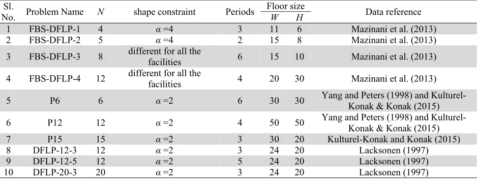
Table 1 gives the list of unequal area dynamic facility layout problems studied in literature either using fixed dimension for facilities or simply aspect ratio constraint or flexible bay structure with aspect ratio constraint. Hence all these problems are taken as good benchmark problems for present study. Note that ‘N’ is the number of facilities, α is the maximum aspect ratio constraint, ‘_Smin’ is the minimum side length

constraint, ‘W’ is the plant length in the x-direction and ‘H’ is the plant length in the y-direction. Table 1 also gives the source information of the problems for detailed data reference. First time, Mazinani et al. (2013) introduced four problems for UA-DFLPs with FBS and named them as1, FBS-DFLP-2, FBS-DFLP-3 and FBS-DFLP-4. Problem FBS-DFLP-1 is 4-facility with 3-period, FBS-DFLP-2 is 5-facilty with 2-period, FBS-DFLP-3 is 8-facility with 6-period and FBS-DFLP-4 is 12-facility with 4-period in the planning horizon.

(14)

assumption of fixed dimensions of facilities and used common maximum aspect ratio as two but their solution approach is not for the flexible bay structure arrangement. Kulturel-Konak and Konak (2015) gave the P15 problem for the UA-DFLPs literature which has 15-facility with 3-period in the planning horizon. Test problems DFLP-12-3, DFLP-12-5 and DFLP-20-3 are from Lacksonen (1997). Problems DFLP-12-3 and DFLP-12-5 have 12-facility with 3 and 5 periods in the planning horizon respectively and DFLP-20-3 has 20-facility with 3 periods in the planning horizon. In these test problems, area of a few facilities changes from period to period in the planning horizon due to induction of new facility and removing the old one. In the present study, P6, P12, P15, DFLP-12-3, DFLP-12-5 and DFLP-20-3are solved with common maximum aspect ratio of two (α= 2) as considered in the literature. In the encoded matrix the number of columns (each row length) in the matrix is taken as (2N-1) for solving all the problems, since the maximum number bays (M) in the layout can be at the most equal to the number of facilities (N). For all data set the number of iterations (epoch length) at each temperature level is taken as N2_.

Table 1

Summary unequal area dynamic facility layout problem data sets

Sl.

No. Problem Name N shape constraint Periods

Floor size

Data reference

W H

1 FBS-DFLP-1 4 α =4 3 11 6 Mazinani et al. (2013)

2 FBS-DFLP-2 5 α =4 2 15 8 Mazinani et al. (2013)

3 FBS-DFLP-3 8 different for all the _facilities 6 15 10 Mazinani et al. (2013)

4 FBS-DFLP-4 12 different for all the _facilities 4 20 30 Mazinani et al. (2013)

5 P6 6 α =2 6 30 30 Yang and Peters (1998) and Kulturel-_{Konak & Konak (2015)}

6 P12 12 α =2 4 50 50 Yang and Peters (1998) and

Kulturel-Konak & Kulturel-Konak (2015)

7 P15 15 α =2 3 30 20 Kulturel-Konak and Konak (2015)

8 DFLP-12-3 12 α =2 3 24 20 Lacksonen (1997)

9 DFLP-12-5 12 α =2 5 24 20 Lacksonen (1997)

10 DFLP-20-3 20 α =2 3 24 20 Lacksonen (1997)

5.1.1 Results and discussion of unequal area DFLPs data set

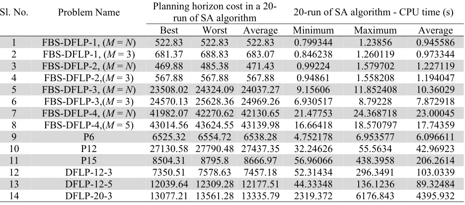
Table 2 shows the 20-run statistical results of all unequal area dynamic facility layout test problems solved using proposed SA algorithm. Table 2 contains best, worst, average of Planning Horizon Cost (PHC) values found, and also it contains minimum, maximum and average CPU timings of SA algorithm. In Table 2, the variability of solution values in the 20 random replications of the SA algorithm for various test problem cases is very small. This can be observed from the very close values of average and best PHC and also, the percentage difference between the best and worst PHCs is almost zero for some of the problems. The computational efficiency of the SA algorithm is also better, as the average computational timing reported for various test case problems are very small, and also the maximum timing reported here is not very high in 20replications.Hence, the proposed SA heuristic method to UA-DFLPs with FBS layout formation is robust one. Mazinani et al. (2013) have solved the problems DFLP-1,

FBS-DFLP-2, FBS-DFLP-3 and FBS-DFLP-4 for given maximum numbers of bays (M). In the present study

also, these problems are solved for given maximum numbers of bays (M) by taking maximum number

(15)

Table 2

Dynamic environment test cases: Planning horizon cost and CPU timing for 20-run of SA applied to UA-DFLP with FBS

Sl. No. Problem Name Planning horizon cost in a 20-_{run of SA algorithm} 20-run of SA algorithm - CPU time (s)

Best Worst Average Minimum Maximum Average

1 FBS-DFLP-1, (M = N) 522.83 522.83 522.83 0.799344 1.23856 0.945586 2 FBS-DFLP-1, (M = 3) 681.37 688.83 683.07 0.846238 1.260119 0.973344 3 FBS-DFLP-2, (M = N) 469.88 485.38 471.43 0.99224 1.579702 1.227119 4 FBS-DFLP-2,(M = 3) 567.88 567.88 567.88 0.94861 1.558208 1.194047 5 FBS-DFLP-3, (M = N) 23508.02 24324.09 24037.27 9.15606 11.852408 10.36029 6 FBS-DFLP-3,(M = 3) 24570.13 25628.36 24969.26 6.930517 8.79228 7.872918 7 FBS-DFLP-4, (M = N) 41982.07 42270.62 42130.65 21.47753 24.368718 23.00045 8 FBS-DFLP-4,(M = 5) 43014.56 43624.55 43139.98 16.66418 18.570797 17.74359 9 P6 6525.32 6554.72 6538.28 4.752178 6.953577 6.096611

10 P12 27130.58 27790.48 27437.35 32.24626 55.5634 42.96923

11 P15 8504.31 8795.8 8666.97 56.96066 438.3958 206.2614

12 DFLP-12-3 7350.51 7578.63 7457.18 52.31434 296.3491 103.0339 13 DFLP-12-5 12039.64 12309.28 12177.51 44.33348 136.1236 89.32484

14 DFLP-20-3 13077.21 13561.28 13335.79 2319.372 6176.843 4395.932

The proposed SA heuristic 20-run best solution in encoded form for different size problems are given in Table 3 and Table 4. The proposed SA heuristic can identify the optimum number bays in the layout for the given data set. In Table 3 it can be noticed that for Mozanani et al.’ (2013) FBS-DFLPs, the planning horizon cost for a given problem size is better when the heuristic itself decides the optimum number of bays in the layout by taking maximum number bays (M) as number of facilities (N), instead of giving the maximum number of bays as input data. The difference in number of optimum bays obtained from the SA heuristic by taking maximum number bays (M) equal to the number of facilities(N) can be noticed in the Table 3 for various size FBS-DFLP problems of Mazinani et al. (2013). For example, FBS-DFLP-1 has 4 bays in all 3 periods for the case of maximum number bays (M = N) equal to the number of facilities. Whereas for the case of given maximum numbers of bays (M =3), SA heuristic obtained the 3 bays for period 1 & 2, and 2 bays for period 3.

Table 3

Best solution found by the proposed SA heuristic for the Mazinani et al. (2013) FBS based test problems Problem Name Periods Best Solution Problem Name Periods Best Solution

FBS-DFLP-1, (M = N)

1 1|2|4|3

FBS-DFLP-3, (M = 3)

1 8-7-6|1-4-5-2|3

2 1|2|4|3 2 8-7-6|1-4-5-2|3

3 1|4|3|2 3 1-4-6|8-7-5-2|3

FBS-DFLP-1, (M = 3)

1 3|4|2-1 4 8-7-6|1-5-4-2|3

2 3|4|2-1 5 8-7-6|1-5-4-2|3

3 2-3|4-1 6 8-4-2|1-5-7-6|3

FBS-DFLP-2, (M = N)

1 4|3|1|5|2

FBS-DFLP-4, (M = N)

1 11|5|7|8-3-12-10-1|6-9|4|2 2 4|3|1|5|2 2 11|5|7|9-3-10-6-1|8-12|4|2 FBS-DFLP-2, (M = 3) 1 2|3|5-1-4 3 11|5|9-10-2|1-6-12-3-8|7|4

2 4|3|5-1-2 4 11|7|1-9-6|2-10-12-3-8|5|4

FBS-DFLP-3, (M = N)

1 8|1|7-4|2-5-6|3

FBS-DFLP-4, (M = 5)

1 11|4|9-12-10-3-8|5-6-1-2|7

2 8|2-4-6|5-7|1|3 2 11|8-9-5-2|12-6-3-10-1|7|4 3 8|2-4-6|5-7|1|3 3 11|1-8-9-3-2|6-12-10-5|7|4

4 8|2-7-6|5-4|1|3 4 11|7|6-10-12-1-2|3-8-9-5|4

5 8|2-7-6|5-4|1|3

(16)

Table 4

Best solution found by the proposed SA heuristic for the non-FBS based test problems Problem

Name Periods Best Solution Problem Name Periods Best Solution

P6

1 2|1-6-5|3-4

P15

1 12-13-6-14-1|15-2-5-3|10-7-11-9-8-4 2 2|1-6-5|3-4 2 10-6-9-1-14|7-12-2-5-13|15-11-8-3-4 3 2|6-5-1|3-4 3 10-6-9-1-13|7-12-5-2-14|15-11-4-8-3 4 2|6-5-1|3-4

DFLP-12-3

1 9-2-7|3-1-6-8|12-10-4|5-11

5 2|6-5-1|3-4 2 7-4|10-6-2-8|12-1-3-9|5-11

6 2|6-5-1|3-4 3 8-3-6-10|9-4-2-1-12|11-5-7

P12

1 7-2|12-1-11|3-9|10-6-4|8-5

DFLP-12-5

1 7-9|4-11-10|2-5-8-12|1-6-3 2 11-7|9-10-1|12-4-6|3-2|8-5 2 6-3-9|4-11-10-12|2-5-8|1-7 3 11-7|3-5|4-1-12|8-10-6|9-2 3 6-7|4-9-5|12-3-10-11-2|8-1 4 10-7|3-5|4-1-12|11-6-9|8-2 4 6-4-3|5-11-10-12|2-9-8|7-1

5 3-6-1|10-9-11-5|12-4-2|8-7

DFLP-20-3

1 5-15-9|17-14-19-1-8|7-16-13-12|6-4-18-20-10|3-11-2 2 8-2-11|12-1-18-20-3|10-19-16-15|13-4-6-7-14|5-9-17 3 11-8-2|20-3-12-10|15-16-18-1-19|14-17-6-4-13|7-9-5

5.1.2 Performance comparison of the proposed SA heuristic for UA-DFLPs with FBS for Mazinani et al. (2013) FBS cases

In this section, effectiveness and efficiency of the proposed SA heuristic is tested with Mazinani et al. (2013) FBS cases. These authors used the GA for solving UA-DFLPs based on FBS. The comparison of planning horizon cost and CPU timings of proposed SA heuristic with GA of Mazinani et al. (2013) are given in Table 5. The proposed SA heuristic method outperformed for all the cases of FBS-DFLPs, when the heuristic itself determines the optimum number of bays in the layout by taking maximum number bays (M) as number of facilities (N), instead of giving the maximum number of bays as input data. Mazinani et al. (2013) have solved FBS-DFLPs for given maximum numbers of bays. In this case also, the proposed SA heuristic has improved the solution value. For the problems DFLP-1 and FBS-DFLP-2, the proposed SA heuristic PHC value is the same as GA of Mazinani et al. (2013). This may be due to the fact that the problem size is small (problem sizes are only 4-facility and 5-facility) and the solution value may be the optimal for this size problems. For big size problems (for 8-facility and 12- facility problems) the proposed SA heuristic has improved the solution value, i.e., for problems FBS-DFLP-3 and FBS-DFLP-4, solution value is improved by+1.97% and +5.09%, respectively. The best solution obtained by the proposed SA heuristic for these data set are given in Table 3 in encoded form.

Table 5

Comparison of planning horizon cost and CPU timing of the proposed SA heuristic for DFLP with FBS based test problems

Problem Name Best planning horizon cost % Impa Average solution time (s)

Mazinani et al. (2013) Proposed SA Mazinani et al. (2013) Proposed SA

FBS-DFLP-1, (M = N) - 522.83 - - 0.95

FBS-DFLP-1, (M = 3) 681.367 681.367 0 7.25 0.97

FBS-DFLP-2, (M = N) - 469.88 - - 1.23

FBS-DFLP-2,(M = 3) 567.875 567.875 0 16.19 1.19

FBS-DFLP-3, (M = N) - 23508.02 - - 10.36

FBS-DFLP-3,(M = 3) 25054.71 24570.13 +1.97 3909.91 7.87

FBS-DFLP-4, (M = N) - 41982.07 - - 23.0

FBS-DFLP-4,(M = 5) 45201.95 43014.56 +5.09 3016.44 17.74

a_{%Imp=100 × (best PHC with FBS-proposed SA best PHC with FBS) /minimum of (best PHC with FBS, proposed SA best PHC with FBS).}

(17)

not directly comparable due to the difference in basic hardware used for testing. The generated solution and CPU timing indicate that the proposed SA heuristic is more effective and efficient for UA-DFLP

with FBS. Also, the best layouts found for FBS-DFLP-1 with M = N, FBS-DFLP-1 with M = 3,

FBS-DFLP-2with M = N, FBS-DFLP-2 with M = 3, FBS-DFLP-3with M = N, FBS-DFLP-3 with M = 3, and FBS-DFLP-4with M = N, FBS-DFLP-4 with M = 5 are shown in Figs. 7 – 9.

Fig. 7.Best layouts found for FBS-DFLP-1 with M = N, FBS-DFLP-1 with M = 3, FBS-DFLP-2 with

M = N and FBS-DFLP-2 with M = 3 problems

3

4

1 5 2

Period = 1

3

4

1 5 2

Period = 2 FBS-DFLP-2, M = N

3 2 1 4 Period = 3 FBS-DFLP-1, M= 3

3

4 1 2

Period = 1

3

4 1 2

Period = 2 FBS-DFLP-1, M= N

Period = 1

1 2 4 3

Period = 2

1

2 4 3

Period = 3

1

4 3 2

FBS-DFLP-2, M = 3

2

3

4 1 5

Period = 1

4

3

2

1 5

Period = 2

8 1

4 6

3 5 2 7

Period = 1

8 6 4 2 7 5

1 3

Period = 2

8 6 4 2 7 5

1 3

Period = 3

8 6 7 2 4 5

1 3

Period = 4

8 6 7 2 4 5

1 3

Period = 5

Fig. 8. (a). Best soltion for FBS-DFLP-3, M = N

8 6 7 2 4 5

1 3

(18)

Fig. 8. Best layouts found for FBS-DFLP-3 with M = N and FBS-DFLP-3 with M = 3 problems

Fig. 9. Best layouts found for FBS-DFLP-4with M = N and FBS-DFLP-4 with M = 5 problems

Fig. 9(a). Best solution for FBS-DFLP-4, M = N

Period = 2

5 11 7 1 6 10 3 9 12 8 4 2

Period = 3

11 5 2 10 9 8 3 12 6 1 7 4

Period = 4

11 7 6 9 1 8 3 12 10 2 5 4

Period = 1

11 5 7 1 10 12 3 8 9 4 6 2

Fig. 9(b). Best solution for

FBS-DFLP-4,M= 5

11

Period = 1

4 8 3 10 12 9 2 1 6 2 4

Period = 2

11 2 5 9 8 1 10 3 6 12 4 7

Period = 3

11 2 3 9 8 1 5 10 12 6

7 4 11 7 9

2 1 12 10

6 3

5 8 4

Period = 4

5 6 7 8 2 4 1 3

Period = 1

7 6 4 1 2 5 8 3

Period = 3

4 6 7 8 2 5 1 3

Period = 4

6 7 8 2 4 1 3

Period = 2

4 6 7 8 2 5 1 3

Period = 5

2 4 8 6 7 5 1 3

Period = 6

Fig. 8. (b) Best solution forFBS-DFLP-3, M = 3

(19)

5.1.3 Performance comparison of the proposed SA heuristic for UA-DFLPs based on FBS with other non-FBS approaches to UA-DFLPs

In this section, the comparison of proposed SA heuristic method is made with various approaches used in the literature to solve UA-DFLPs which are not based on FBS. Lacksonen (1997) uses pre-processing and branch and bound strategy to solve aspect ratio constraint problems DFLP-12-3, DFLP-12-5 and DFLP-20-3. Researchers (Dunker et al., 2005; McKendall & Hakobyan, 2010; Derakhshan Asl & Wong 2017) used various meta-heuristics like combined GA and dynamic programming, boundary search and tabu search heuristics, and particle swarm optimization to solve fixed shape facilities problem of P6 and P12. Kulturel-Konak and Konak (2015) apply large scale simulated annealing algorithm as solution methodology to solve P6, P12, P15, DFLP-12-3, DFLP-12-5 and DFLP-20-3 problems with aspect ratio constraint for the facilities and without FBS in layout. Table 6 gives the comparison of PHC of proposed FBS based SA heuristic with other meta-heuristics used for solving UA-DFLPs without bays formation in the layout. The best solution obtained by the proposed SA heuristic for these data set are given in Table 4 in encoded form. When the proposed SA heuristic approach to UA-DFLPs with FBS is compared with the non-FBS based approaches, results are not far from earlier best known results reported in the literature, even though FBS representation is more constrained than non-FBS approaches.

Table 6

Planning horizon cost comparison of proposed FBS based SA heuristic with other non-FBS based approaches reported in the literature for UA-DFLPs

Problem Na

m

e

L

acksonen (199

7)]

Y

ang

and

Pete

rs

(1

998

)

Dunke

rs

et

al.

(

20

05)

M

cKendall an

d

Hakob

ya

n

(2

010

)

De

ra

kh

shan

A

sl and _Wong ₍₂017

)

K

ulturel-Konak and Konak (2

015

)

Be

st-kno

w

n

for

non-FBS

Appr

oach

Propo

se

d

SA

w

ith

FBS

(%

) Imp

ov

er

no

n-FBS

P6 - 7657 6906.5 6906.5 6763.76 5899.41 5899.41 6525.32 -10.61

P12 - 30344 29098.5 28845.5 28826.67 25828.18 25828.18 27130.58 -5.04

P15 - - - 8376.64 8376.64 8504.31 -1.52

DFLP-12-3 7094 - - - - 6622.82 6622.82 7350.51 -10.99

DFLP-12-5 12271 - - - - 11412.39 11412.39 12039.64 -5.50

DFLP-20-3 12903 - - - - 12148.60 12148.60 13077.21 -7.64

% Imp=100 × (best PHC for non-FBS-proposed SAPHC for FBS) /minimum of (best PHC for non-FBS, proposed SA PHC for FBS)

5.1.4 Proposed SA heuristic computational effort discussions

(20)

Table 7

Comparison of proposed FBS based SA heuristic average CPU timings (seconds) with the other approaches CPU timings for UA-DFLPs

Problem Name

Lacksonen (1997)

Dunkers et al. (2005)

McKendall and Hakobyan

(2010)

Asl and Wong (2017)

Kulturel-Konak and Konak

(2015)

Proposed SA average

CPU time

P6 - 1764 1666.2 2354.58 1716 6.10

P12 - 9600 4923 11105.56 28012 42.97

P15 - - - - 11242 206.26

DFLP-12-3 192 - - - 2981.19 103.03

DFLP-12-5 45196 - - - 3951.35 89.32

DFLP-20-3 69945 - - - 6342.37 4395.93

5.2 Proposed SA heuristic for equal area DFLPs data set

In the literature, equal area-DFLPs are studied with discrete space dynamic QAP model. These equal area DFLPs are used in the proposed continuous space SA heuristic, since the discrete space equal area DFLPs are the specific case of continuous space UA-DFLP with FBS when area and aspect ratio of all facilities are set to one. Summary of data sets for equal area dynamic facility layout problems is given in Table 8. Problem R6 is 6-equal area facility problem and is taken from Rosenblat (1986). Problem CV9 is from Conway and Venkataramanan (1994) which is 9-equal area facility problem. Problem Y9 is also 9-equal area facility problem and it is from Yaman et al. (1993). All 9-facility data sets use discrete 3×3 location grid for locating the facilities. Chan et al. (2002) provided the part handling factor data.

Table 8

Summary of equal area dynamic facility layout problem data sets

Sl.

No. Problem Name N Shape constraint Periods

Floor size

Data reference

W H

1 R6 6 _Smin₌₁ ₅ ₃ ₂ _{Rosenblat (1986)}

2 CV9 9 _Smin

=1 5 3 3 Conway and Venkataramanan (1994)

3 Y9 9 _Smin

=1 5 3 3 Yaman et al. (1993)

4 Y9-part 9 _Smin₌₁ ₅ ₃ _{3 Yaman et al. (1993) and Chan et al.(2004)}

5 C9-S1 9 _Smin₌₁ ₅ ₃ ₃ _{Chan et al.(2004)}

6 C9-S1-part 9 _Smin

=1 5 3 3 Chan et al.(2004)

7 C9-S2 9 _Smin

=1 5 3 3 Chan et al.(2004)

8 C9-S2-part 9 _Smin₌₁ _{5 3}₃ _Chan_et_al.(2004)

Chan et al. (2004) solved Yaman et al. (1993) problem using the part handling data in dynamic environment. In this paper, Yaman et al.’s (1993) Y9 problem studied with part handling factor is denoted as Y9-part. Chan et al. (2004) generated two 9-facility equal area problem data which are named here as C9-S1 and C9-S2 and data of these problems are also studied with part handling factor. The problems S1 and S2 studied with consideration of part handling factor are named as S1-part and C9-S2-part, respectively. All these authors used the discrete space QAP model and solved with various exact and heuristic methods. In the present study, the above equal area-DFLPs are solved with proposed SA heuristic for UA-DFLPs with FBS. In order to use the equal area data in continuous space MILP model

of UA-DFLP with FBS, we assumed unit area (A=1) for each facility and minimum side length of each

facility as one (_Smin_{=1). For nine facilities problems, the plant floor size of 3×3 is considered (i.e.,}_W=

(21)

Table 9

20-run PHC and CPU timing of proposed SA heuristic applied to equal area DFLP data set

Sl. No. Problem Name Planning horizon cost in a 20-run of SA algorithm 20-run of SA algorithm - CPU timings in (s)

Best Worst Average Minimum Maximum Average

1 R6 71187 72803 71634.1 2.33126 5.040148 3.403723

2 CV9 607427 612222 609476.6 12.96562 14.93574 13.94695

3 Y9 13700 15490 14334 27.88492 29.31597 28.52374

4 Y9- part 44895 47841 46813.6 10.76329 14.16162 12.48683

5 C9-S1 289900 309090 303685.1 26.23782 28.63932 27.42123

6 C9-S1-part 608400 621003 615232 12.37152 14.52916 13.56194

7 C9-S2 333701 350089 339598.6 11.79689 14.84242 13.34262

8 C9-S2- part 708181 719738 711857.3 11.2186 14.58263 13.61192

Table 10

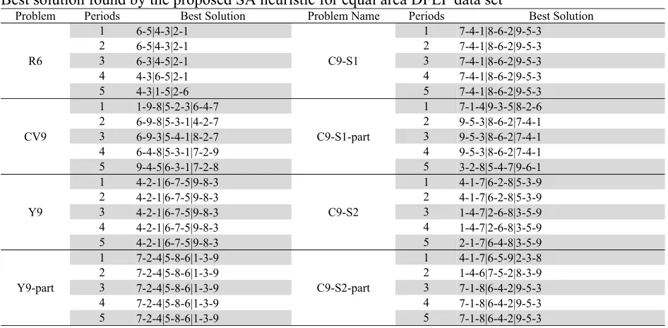
Best solution found by the proposed SA heuristic for equal area DFLP data set

Problem Periods Best Solution Problem Name Periods Best Solution

R6

1 6-5|4-3|2-1

C9-S1

1 7-4-1|8-6-2|9-5-3

2 6-5|4-3|2-1 2 7-4-1|8-6-2|9-5-3

3 6-3|4-5|2-1 3 7-4-1|8-6-2|9-5-3

4 4-3|6-5|2-1 4 7-4-1|8-6-2|9-5-3

5 4-3|1-5|2-6 5 7-4-1|8-6-2|9-5-3

CV9

1 1-9-8|5-2-3|6-4-7

C9-S1-part

1 7-1-4|9-3-5|8-2-6 2 6-9-8|5-3-1|4-2-7 2 9-5-3|8-6-2|7-4-1 3 6-9-3|5-4-1|8-2-7 3 9-5-3|8-6-2|7-4-1 4 6-4-8|5-3-1|7-2-9 4 9-5-3|8-6-2|7-4-1 5 9-4-5|6-3-1|7-2-8 5 3-2-8|5-4-7|9-6-1

Y9

1 4-2-1|6-7-5|9-8-3

C9-S2

1 4-1-7|6-2-8|5-3-9 2 4-2-1|6-7-5|9-8-3 2 4-1-7|6-2-8|5-3-9 3 4-2-1|6-7-5|9-8-3 3 1-4-7|2-6-8|3-5-9 4 4-2-1|6-7-5|9-8-3 4 1-4-7|2-6-8|3-5-9 5 4-2-1|6-7-5|9-8-3 5 2-1-7|6-4-8|3-5-9

Y9-part

1 7-2-4|5-8-6|1-3-9

C9-S2-part

1 4-1-7|6-5-9|2-3-8 2 7-2-4|5-8-6|1-3-9 2 1-4-6|7-5-2|8-3-9 3 7-2-4|5-8-6|1-3-9 3 7-1-8|6-4-2|9-5-3 4 7-2-4|5-8-6|1-3-9 4 7-1-8|6-4-2|9-5-3 5 7-2-4|5-8-6|1-3-9 5 7-1-8|6-4-2|9-5-3

5.2.1 Results and discussion of equal area DFLPs data set

Table 9 shows the 20-run statistical results of all equal area dynamic facility layout test problems solved using proposed SA heuristic. In Table 9, the variability of solution values in the 20 random replications of the SA heuristic for test cases is small. This can be observed from the very close average and best PHC values. The computational efficiency of the SA algorithm is also better, as the average computational timing reported for various test case problems are very small. Hence, the proposed SA heuristic method to solve equal area DFLPs is robust one. Also, the best solution found by the proposed SA heuristic for equal area DFLP data set are shown in Table 10.

5.2.2 Performance comparison of equal area dynamic facility layout problems data set

(22)

consideration of part handling factor. Hence, the consideration of part handling factor has the impact on the arrangement of facilities in the layout solution. The difference in solution (i.e., change in layout configuration) can be noticed from Table 10, which contains the best solution with and without consideration of part handling factor in encoded form. For R6, CV9 and C9-S1 problems, the proposed SA heuristic has given almost the same solution values compared with the best solution values reported in the literature. The proposed SA heuristic method has improved the solution value for Y9 and Y9-part problems as compared with the best known solution value in literature (i.e., +6.35% and +1.69% respectively). For C9-S1-part, C9-S2 and C9-S2-part problems, the proposed SA heuristic method has given the little inferior PHC than the best solution reported in the literature. In general, the performance of proposed SA heuristic to equal area DFLPs is better.

Table 11

Comparison of proposed SA heuristic solution value with the other adaptive approaches solution values for equal area DFLPs

Problem name Rosenblatt (1986) _{Venkataramanan (1994)}Conway and Chan et al. ₍₂₀₀₄₎ Mazinani et al. (2013) Best Known Proposed SA _best % Imp

R6 71178 71178 - 71178 71178 71187 -0.01

CV9 - 608904 - 606762 606762 607427 -0.11

Y9 - - 14570 - 14570 13700 +6.35

Y9-part - - 45655 - 45655 44895 +1.69

C9-S1 - - 289900 - 289900 289900 0

C9-S1-part - - 605200 - 605200 608400 -0.53

C9-S2 - - 324360 - 324360 333701 -2.88

C9-S2-part - - 698351.4 - 698351.4 708181 -1.41

% Imp =100 × (best known PHC value - proposed SA heuristic PHC value) divided by minimum of (best known PHC value, proposed SA heuristic PHC value)

6.Conclusions

In this paper, SA heuristic method for UA-DFLP with FBS has been proposed. The concept of part handling factor has included in the continuous space MILP model of Mazinani et al. (2013) to compute the actual flow volume between facilities in different periods of the planning horizon. The effectiveness and efficiency of SA heuristic have been tested with wide range of dynamic unequal area and equal area facility layout problems available in the literature. The proposed SA algorithm has given the better or the same solution for FBS based test problems as compared with the best-known reported in the literature. The CPU timings of the proposed SA algorithm are superior to the other meta-heuristic in the literature. The proposed SA heuristic procedure is highly efficient to solve DFLP with FBS. The standard UA-DFLPs available in the non-FBS literature have been tested with the proposed SA heuristic. The SA heuristic solution is not significantly different from the best solution reported in the literature for non-FBS approaches. The proposed SA heuristic to UA-DFLPs creates the bays in layout, while other approaches reported in the literature used to solve standard UA-DFLPs does not create bays in the layout. The result of proposed SA heuristic to continuous space MILP model is almost the same as the result of other heuristics used for discrete space dynamic QAP model. Hence, the proposed SA heuristic method is a universal method as it can solve both unequal area and equal area dynamic environment facility layout problems with flexible bays in the layout. Future research work can be in the direction of considering multi-objectives in the SA heuristic method to UA-DFLP with FBS so that the intervention of decision maker requirements can be incorporated. In the present study, only feasible configuration changes are considered in the SA heuristic, in futu