Ocean Sci., 10, 39–48, 2014 www.ocean-sci.net/10/39/2014/ doi:10.5194/os-10-39-2014
© Author(s) 2014. CC Attribution 3.0 License.
Ocean Science
Open Access
Enhancing the accuracy of automatic eddy detection and the
capability of recognizing the multi-core structures from maps of sea
level anomaly
J. Yi1, Y. Du1, Z. He2,3, and C. Zhou1
1State Key Laboratory of Resources and Environmental Information System, Institute of Geographic Sciences and Natural
Resources Research, Chinese Academy of Sciences, Beijing 100101, China
2State Key Laboratory of Tropical Oceanography (LTO), South China Sea Institute of Oceanology, Chinese Academy of
Sciences, Guangzhou 510301, Guangdong, China
3College of Ocean and Earth Sciences, Xiamen University, Xiamen 361005, China
Correspondence to: Y. Du ([email protected])
Received: 5 April 2013 – Published in Ocean Sci. Discuss.: 29 April 2013
Revised: 2 December 2013 – Accepted: 7 January 2014 – Published: 10 February 2014
Abstract. Automated methods are important for automati-cally detecting mesoscale eddies in large volumes of altime-ter data. While many algorithms have been proposed in the past, this paper presents a new method, called hybrid detec-tion (HD), to enhance the eddy detecdetec-tion accuracy and the ca-pability of recognizing eddy multi-core structures from maps of sea level anomaly (SLA). The HD method has integrated the criteria of the Okubo–Weiss (OW) method and the sea surface height-based (SSH-based) method, two commonly used eddy detection algorithms. Evaluation of the detection accuracy shows that the successful detection rate of HD is
∼96.6 % and the excessive detection rate is∼14.2 %, which outperforms the OW and those methods using SLA extrema to identify eddies. The capability of recognizing multi-core structures and its significance in tracking eddy splitting or merging events have been illustrated by comparing with the detection results of different algorithms and observations in previous literature.
1 Introduction
Mesoscale eddies play an important role in ocean circula-tion as well as in heat and mass transport (McWilliams, 2008; Nencioli et al., 2010). With the development of obser-vation technology, automated detection methods are essen-tial for understanding the complex movements and dynamic
characteristics of mesoscale eddies in large volumes of al-timeter data. In Eulerian schemes (distinguished from La-grangian detection schemes using drifting trajectory data (Dong et al., 2011)), existing eddy detection methods can be categorized into three classes: (1) those based on a physical parameter, (2) those based on flow geometry, and (3) those based on sea surface height anomaly (SSHA).
locate the eddies or underestimate the dimensions (Basdevant and Philipovitch, 1994; Doglioli et al., 2007; Henson and Thomas, 2008; Isern-Fontanet et al., 2003a).
To improve eddy detection, some novel approaches based on flow geometry characteristics were developed. The winding-angle (WA) approach first proposed by Ari Sadar-joen and Post (2000) is a representative that identifies ed-dies by clustering closed or spiral streamlines. Chaigneau et al. (2008) adapted this approach by using sea level anomaly (SLA) local extrema as potential eddy centers and the out-ermost streamlines as corresponding boundaries. Nencioli et al. (2010) argued that this adaption incorporated a physical quantity (SLA) and thus should be regarded as a hybrid ap-proach. Consequently, they further developed a pure flow geometry-based, or vector geometry-based (VG) approach, which identifies eddies only by the geometry characteristics of velocity fields and is independent from parameters derived using velocity derivatives as well as from the SLA field (Nen-cioli et al., 2010). However, the specification and sensitivity test of two additional parameters that are used for searching eddy centers complicate the identification procedure.
The third category directly uses SSHA or SLA for eddy identification in which a threshold is nevertheless always re-quired to delimit eddy dimensions. Fang and Morrow (2003) used a 10 cm threshold to identify the large eddies in the South Indian Ocean. Chaigneau and Pizzaro (2005) chose 6 cm to detect eddies in the region west of South America, and Wang et al. (2003) selected 7.5 cm for eddy identification in the South China Sea (SCS). In 2010, Chelton et al. (2011) proposed a sea surface height-based (SSH-based) method for global studies and eliminated the threshold dependency on SSHA. However, this method relies on other thresholds (e.g., area and horizontal scale) that were specified in its detection criteria to determine the eddy boundaries, and may yield ed-dies with more than one local extremum, which are referred to as multi-core structures in this paper.
Multi-core structures exist in the vicinity of mutual inter-actions between eddies, so that identifying and tracking them may allow one to understand how eddies interact with each other, how they split or merge, and how the energy trans-fers and exchanges. However, few studies have developed algorithms capable of detecting and tracking them. Chelton et al. (2011) tried splitting the multi-core structures, only to find extra induced problems in tracking them, so they even-tually abandoned the splitting procedure. This paper presents a hybrid detection method (HD) that attempts to identify and characterize the multi-core structures and lays the founda-tion for further tracking the evolufounda-tion processes correctly. A companion tracking method that addresses the difficulties in tracking multi-core structures will be elaborated in another paper. This paper is mainly focused on the discussion of the new detection method and its performance.
The detection accuracy defines the quality of eddy iden-tification algorithms and is a necessary evaluation criterion
ods presents a promising avenue to improving the perfor-mance of detection algorithms, for it tries to make the best of the advantages and minimize the disadvantages of each sin-gle method. In previous literature, the adapted WA method (Chaigneau et al., 2008) incorporated SLA extrema to make the algorithm more simple and efficient. Morrow et al. (2004) combined additional SLA criteria to reduce excessive detec-tions of the Q-parameter approach. In this paper, the HD method is developed with the integration of the OW method and the SSH-based method; it combines theWparameter cri-terion and SLA local extrema to detect eddy centers and uses SLA contours to delineate the dimensions of eddies. An ob-jective validation protocol that has been used by Chaigneau et al. (2008) and Nencioli et al. (2010) is adopted to measure the detection accuracy of the HD method. Meanwhile, the de-tection results of different algorithms are compared to exam-ine the performance of HD and the ability of characterizing multi-core structures. Nan et al. (2011)’s study of three an-ticyclonic eddies among which splitting and merging events had been observed is used to verify HD’s detection results and to demonstrate the significance of recognizing multi-core structures.
The rest of the paper is organized as follows: Sect. 2 in-troduces the altimetry data and the detailed procedures of the HD method; Sect. 3 presents the results and discussion of HD’s detection evaluation, method comparisons, and histor-ical verifications; and the final section provides the conclu-sions.
2 Data and method
2.1 Altimetry data
As combining data from different satellite missions improves the estimation of mesoscale signals (Le Traon and Dibar-boure, 1999; Chelton and Schlax, 2003; Pascual et al., 2006), the SLA data set (October 1992 to April 2012) of the AVISO (http://www.aviso.oceanobs.com) Reference Series delayed-time aldelayed-timeter products merging TOPEX/Poseidon (T/P), Jason-1, ERS-1/2, and Envisat data (Ducet et al., 2000) was used to identify mesoscale eddies. This merged altimeter data set consists of weekly SLA maps computed with respect to a seven-year mean and resampled on a 1/3◦×1/3◦Mercator grid.
2.2 Eddy detection methodology
J. Yi et al.: Enhancing the accuracy of automatic eddy detection 41
24 1
Figure 1. Detailed procedures of step 1. Procedure in the box with dashed border is adaptable 2
according to the data quality and the eddy characteristics of different study regions. 3
4 5
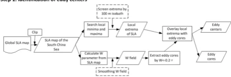
Fig. 1. Detailed procedures of step 1. Procedure in the box with
dashed border is adaptable according to the data quality and the eddy characteristics of different study regions.
the new method thus has three steps: (1) identify eddy cen-ters; (2) find eddy boundaries; and (3) distinguish multi-core structures.
2.2.1 Step 1: a hybrid way to identify eddy centers
The velocity field within an ocean eddy is dominated by ro-tation, corresponding to the negativeW values in the OW method that can be used to recognize where eddies exist. Among the studies using the OW method, many adopted the criterionW<−0.2σw(σwis the spatial standard deviation of W) for detecting ocean eddies from altimetry data, but this criterion usually brings undesirable noise into the data and causes false detections (Isern-Fontanet et al., 2006; Henson et al., 2008; Xiu et al., 2010).
Having an SLA maximum (or minimum) inside the eddy-dominant region is another essential character of ocean ed-dies, which has been adopted in the WA method, the SSH-based method as well as other eddy detection methods; here-after they are all referred to as the SLA extremum-based methods. Following the definition that “a vortex exists when instantaneous streamlines mapped onto a plane normal to the vortex core exhibit a roughly circular or spiral pattern [. . . ]” (Robinson, 1991), Chaigneau et al. (2008) improved the WA method by incorporating the SLA extrema criterion. Besides, the threshold-free SSH-based method developed by Chelton et al. (2011) for global eddy detection also required quali-fied eddies to contain at least one local minimum or maxi-mum. However, it should be noted that noise on SSHA or SLA fields may form false maxima and minima and there-fore could induce spurious detection of extrema.
Based on these definitions of an eddy and the correspond-ing eddy detection methods developed in previous studies, we argue that an eddy should have a core area where the velocity field is dominated by rotation and the streamlines show a circular or spiral pattern, and an SLA maximum or minimum inside. So, this study developed a hybrid detec-tion algorithm that has integrated both theW parameter cri-terion and SLA extrema cricri-terion to effectively reduce ex-cessive detections and enhance the detection accuracy. Here, to avoid confusion, the local extrema of SLA in eddies are
25 1
Figure 2. Detailed procedures of step 2. 2
3
Fig. 2. Detailed procedures of step 2.
referred to as “eddy centers” while the connected regions whereW<−0.2σware referred to as “eddy cores”.
Figure 1 shows the details of step 1. Each global SLA map is first clipped to the study region (e.g., the South China Sea). Then, the program calculates theW parameter and searches for local extrema within that clipped SLA. Regions where W<−0.2σware extracted as eddy cores. Meanwhile, the lo-cal SLA extrema are searched out by running a 3×3 grid window (the smallest scale) on an SLA map. If the central point is a maximum or minimum of the window, then it rep-resents a local extremum, and the extremum will be qualified as an eddy center only if it is located in a core area.
In this procedure, extra restrictions can be added based on the data quality of different study regions. In the South China Sea, for example, eddy centers located over water depths shallower than 100 m are removed due to alias from tides and internal waves contained in the SLA data over the shal-low shelf area (Yuan et al., 2006). In addition, a smoothing algorithm, like a half-power filter (Chelton et al., 2011) or Hanning filter (Penven et al., 2005), can also be added to reduce the noise in theW field, but to avoid removing any physical information, this study applied no smoothing algo-rithms.
2.2.2 Step 2: definition and extraction of eddy boundaries
Existing algorithms lack a consistent definition of eddy boundaries, and detection results can vary significantly de-pending on the rules for extracting the boundary (Nencioli et al., 2010). The OW method defines enclosed regions as eddies where W values satisfy the criterion. However, this criterion is restricted to the core of the vortices and may un-derestimate eddy dimensions (Basdevant and Philipovitch, 1994). The WA method and the VG method represent eddy boundaries by streamlines, which make better approximation of eddy shapes, and given the good agreement with stream-lines, the SSH-based method takes the outermost closed con-tours of SSHA as eddy boundaries. So, in the HD method, we also use SLA contours to represent eddy boundaries, but the “outermost” criterion is further refined to make the boundary extraction more sensible. The detailed procedures are shown in Fig. 2.
26 2
Figure 3. Detection results of different contour intervals. The eddy boundary is determined by 3
the HD algorithm which has combined OW criterion and SSH-based criterion. 4
5
Fig. 3. Detection results of different contour intervals. The eddy boundary is determined by the HD algorithm that has combined the OW
criterion and the SSH-based criterion.
interiors (Chelton et al., 2011). The smaller increment is pre-ferred for it provides a better approximation of eddy dimen-sions. We carefully checked the detection results of different contour intervals and found that contours with 1 cm incre-ments may underestimate the dimensions of eddies (Fig. 3a). We also found that 0.25 cm improves the boundary approx-imation, but the time consumption increases significantly when the increment becomes much smaller. So, the incre-ment of 0.5 cm represents a compromise choice. Contours that are unclosed or have a diameter greater than 500 km are removed from the data set.
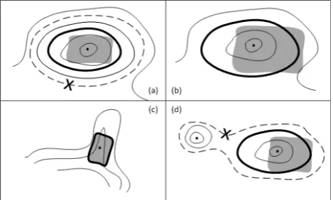
Second, the eddy centers and cores identified in step 1 are combined to decide which contours surrounding the eddy centers should be their corresponding boundaries. For each eddy center, the smallest contour that encompasses its core area is regarded as the qualified boundary. This definition im-proves the approximation of eddy shape while choosing the outermost closed contours, as boundaries tend to enlarge the dimensions. Figure 4a illustrates the difference between the two criteria.
It is noteworthy that some special situations may occur during the process of extracting eddy boundaries. For in-stance, it is possible that eddies may have no contours com-pletely containing their core areas (Fig. 4b), or even no closed contours around the eddy center (Fig. 4c). In the former case, eddy boundaries are defined by the outermost closed contour that intersects the core areas, while in the lat-ter case, the eddy dimensions are defined by the core, just as the OW method does. While some may argue about the existence of these weak eddies in the latter case, this study retains them during the identification process, as they may be in the immature or unstable stages (e.g., forming or disap-pearing) of their evolution processes and removing them will break a coherent process into discrete evolution pieces when they are tracked. Figure 4d illustrates another case that eddy boundaries contain extra local extrema but not qualified eddy centers. In such cases, the boundaries improperly enlarge the dimensions, and so are removed before the boundary extrac-tion procedure. Moreover, contours containing two or more eddy centers of opposite polarities are also discarded in this study.
We summarize all the criteria or constraints used for de-tecting eddy centers and boundaries in the HD method as follows:
27 1
Figure 4. Possible situations in extracting eddy boundary. The contours are represented by the 2
thin solid lines while the eddy boundary is underlined by the thick solid line. Eddies’ core 3
areas are symbolized by grey polygons. And the dashed lines denote the outermost closed 4
contours. 5 6
Fig. 4. Possible situations in extracting an eddy boundary. The
con-tours are represented by the thin solid lines, while the eddy bound-ary is underlined by the thick solid line. Eddy core areas are sym-bolized by grey polygons, and the dashed lines denote the outermost closed contours.
1. W<−0.2σwfor detecting eddy core areas;
2. 3×3 grid moving window for searching SLA maxima and minima;
3. only those SLA maxima or minima that lie within core areas are qualified as eddy centers;
4. eddy centers located over shallow depths (taken to be 100 m in the SCS) are discarded;
5. the contours of SLA are generated with increments of 0.5 cm;
6. unclosed contours or diameter greater than 500 km are discarded;
7. the minimum closed SLA contours that encompass eddy core areas are defined as qualified boundaries; 8. if no closed contours completely contain the core
ar-eas, then take the outermost closed contours that inter-sect with the core areas as eddy boundaries;
J. Yi et al.: Enhancing the accuracy of automatic eddy detection 43
28 1
Figure 5. Identification of multi-core structures and boundary restorations. The contours are 2
represented by thin solid lines. The grey polygons represent eddies’ core areas. 3
4 5
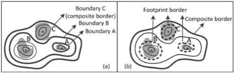
Fig. 5. Identification of multi-core structures and boundary
restora-tions. The contours are represented by thin solid lines. The grey polygons represent eddy core areas.
2.2.3 Step 3: multi-core recognition and boundary restoration
The multi-core structures of eddies, which have two or more closed eddies of the same polarity within the boundaries, rep-resent the important transitional stages of their lives in which component eddies may experience splitting, merging or other energy-transferring interactions. They were little mentioned and had no clear definition in previous studies. The SSH-based criteria can yield multi-core structures, but they fail to characterize their shapes and track their evolution processes. The HD method developed in this study attempts to recog-nize eddy multi-core structures fully so that we can address the difficulties they bring to tracking algorithms.
After step 2, every eddy center has been associated with a unique boundary. This step further defines that if the bound-ary of an eddy contains other eddy centers, it reveals a multi-core structure, and the boundary is taken as the “compos-ite” border of the whole structure (Fig. 5a). If there are mul-tiple composite borders, the algorithm just retains the out-ermost one. The borders of inner component eddies, which we called “footprint” borders, are defined by the outermost closed contours that only contain one eddy center. In brief, HD characterizes the spatial domain of multi-eddy structures and included eddies by the composite borders and the foot-print borders, respectively.
After recognizing multi-core structures, the procedure needs to check every eddy’s boundary and extract the com-posite borders and footprint borders. For example, in Fig. 5a, after step 2, sub-eddy C’s boundary was found to be the out-ermost boundary containing sub-eddies A and B, and there-fore it should be recognized as the composite border. Sub-eddy B’s boundary conflicts with the definition of a footprint border for it contains eddy A, so that subsequent restorations are needed to assign the correct boundary. Figure 5b shows the correct borders of the multi-core structure and its compo-nent eddies after the boundary restoration based on the defi-nitions of composite borders and footprint borders.
3 Results and discussion
3.1 Detection accuracy in the South China Sea
The accuracy is an important measure of the eddy iden-tification quality. According to the validation protocol in Chaigneau et al. (2008), two quantities can be used to eval-uate the accuracy of identification algorithms: the success of detection rate (SDR) and the excess of detection rate (EDR). Definitions are shown as follows:
SDR=Nc Ne
(1)
EDR=Nom Ne
(2) WhereNccorresponds to the number of the eddies identified
by both experts and the automated algorithm,Necorresponds
to the number of the eddies only identified by the experts, and Nomcorresponds to the number of the eddies only identified
by the algorithm.
This study randomly selected ten SLA maps of SCS (100◦E–125◦E; 5◦N–26◦N) from 1992 to 2012 to compute SDR and EDR of the HD method. Five experts were invited to manually detect eddies on these sample maps. On each map, only eddies recognized by at least three experts were counted in the detection result used for accuracy evaluation. As subjective bias usually exists among the experts, estimat-ing the uncertainty of each derived manual detection result is necessary to understand how difficult it may be to correctly identify eddies from a specific SLA map, and to what extent the detection error of automatic algorithms can be tolerated. Here, we introduce the ratio of inconsistency (RI) to measure the uncertainty of expert results. The definition is as follows:
RIi=
|Ni−Nce|
Nce
(3) Where RIi denotes the inconsistency rate of experti.Ni is the number of eddies identified by expert i andNce is the
number of eddies that are commonly recognized by at least three experts.Nimay be less thanNce, and so to avoid
nega-tive values we only compute the absolute value of RI. Figure 6a shows the comparison between expert detec-tion (circles) and the HD result (dots) on 9 May 2007, SCS. There are 25 eddies (Ne=25) detected by the experts on this
data set (12 cyclonic and 13 anticyclonic). Four eddies were overly detected (Nom=4) and one was missed (Nc=24) by
the HD. So, according to the definition, SDR = 96.0 % and EDR = 16.0 % in this experiment.
1 2 3 4 5 6 7 8 9 10
Date 13/07/1994 03/07/1995 17/07/1996 21/01/1998 08/09/1999 16/05/2001 09/10/2002 12/11/2003 11/05/2005 09/05/2007 Average
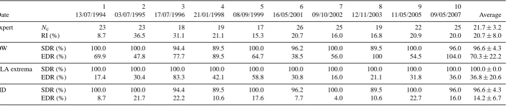
expert Nc 23 23 18 19 17 26 25 19 22 25 21.7±3.2
RI (%) 8.7 36.5 31.1 21.1 15.3 20.7 16.0 16.8 20.9 20.0 20.7±8.0
OW SDR (%) 100.0 100.0 94.4 89.5 100.0 96.2 100.0 89.5 100.0 96.0 96.6±4.3
EDR (%) 69.9 47.8 77.7 89.5 64.7 38.5 56.0 100 54.5 104.0 70.3±22.2
SLA extrema SDR (%) 100.0 100.0 100.0 100.0 100.0 100.0 100.0 100.0 100.0 100.0 100.0±0.0
EDR (%) 17.4 30.4 83.3 42.1 58.8 30.8 16.0 21.1 31.8 36.0 36.8±20.6
HD SDR (%) 100.0 100.0 94.4 89.5 100.0 96.2 100.0 89.5 100.0 96.0 96.6±4.3
EDR (%) 8.7 21.7 22.2 10.6 17.6 7.7 4.0 10.6 22.7 16.0 14.2±6.7
29 1
2
Figure 6. (a) Comparisons between experts’ detection result and HD’s result on May 9th, 2007.
3
The 100 m depth isobath is delineated by the black solid line. The circles represent eddies 4
identified by experts while the dots represent the ones identified by HD. These detection 5
results are superposed on SLA field of that date. (b) One missed eddy in HD’s result. Red 6
triangles represent the SLA local extrema, and the grey polygons represent eddies’ core areas. 7
(c) One over-detected eddy that constitutes a multi-core structure. The composite borders are 8
delineated by the solid lines and the footprint borders by the dashed lines. (d) The other 9
over-detected eddy located near the border of study region. 10
11
12
Fig. 6. (a) Comparisons between experts’ detection result and HD’s
result on 9 May 2007. The 100 m depth isobath is delineated by the black solid line. The circles represent eddies identified by experts, while the dots represent the ones identified by HD. These detec-tion results are superposed onto the SLA field of that date. (b) One missed eddy in HD’s result. Red triangles represent the SLA lo-cal extrema, and the grey polygons represent eddy core areas. (c) One over-detected eddy that constitutes a multi-core structure. The composite borders are delineated by the solid lines and the foot-print borders by the dashed lines. (d) The other over-detected eddy located near the border of the study region.
an upper bound of the acceptable tolerance for detection er-rors. The detection accuracy of the OW method and the SLA extremum-based method were also presented in Table 1 for comparison.
The results show that all the detection methods have rela-tively high SDRs. The methods using SLA local extrema to identify eddies maintain 100 % SDR on every map, which confirms that the SLA local extrema are necessary evidence for the existence of eddies. The SDRs of the OW method and the HD method are both equal to ∼96.6 % on aver-age;∼3.4 % eddies failed to be recognized by either OW or HD. Further examination reveals that these overlooked ed-dies were not located in the intense vorticity regions (where W<−0.2σw)but nearby (Fig. 6b), and were hence excluded from the qualified eddy centers identified by the HD method.
Second, EDR of different methods in the results varies wildly. The EDR of OW is high at ∼70.3 % on average and even exceeds 100 % in single experiments (e.g., on 19 May 2007), which is evidence of the over-detection weak-ness of the OW method. The average EDR of the SLA extremum-based method (∼36.8 %) is much lower than that of OW, which agrees with the validation results in Chaigneau et al. (2008) and confirms that the WA method is more ac-curate than OW. The HD method has the lowest EDR in single experiments and on average. This result substantiates that the integration of the OW and SSH-based criteria effec-tively improves the detection accuracy. In addition, the av-erage EDR of HD (∼14.2 %) is under the tolerance bound (20.7 %) of acceptable detection errors, which further con-firms the feasibility as an automatic algorithm in practical applications. In-depth investigation shows that the∼14.2 % excessively detected eddies are mainly ascribed to two rea-sons: most of them (1) constitute a part of multi-core struc-tures (Fig. 6c); or (2) are located near the boundary of the study region (Fig. 6d). Both cases tend to be overlooked in manual detection.
Another analysis using the receiver operating character-istic (ROC) graphs (Fawcett, 2006) was also performed to compare the detection accuracy of different methods, and the analysis result (Fig. 7) reconfirms the good performance of the HD method over the OW method and the SLA extremum-based method. Most of the ROC points of the HD method are located near the top-left corner, which represents perfect de-tection accuracy. The OW method’s performance is the poor-est as most of the ROC points are clustered in the top-right corner.
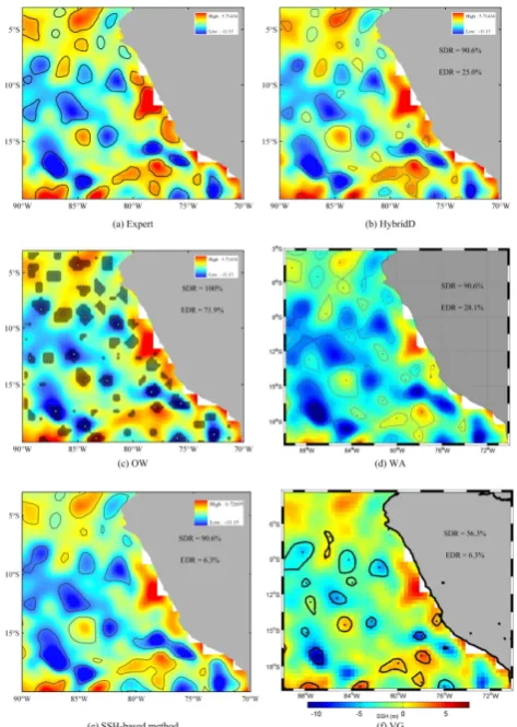
3.2 Detection results in the Eastern South Pacific Ocean
J. Yi et al.: Enhancing the accuracy of automatic eddy detection 45
30 1
Figure 7. the ROC analysis result of the detection methods in the SCS. 2 Fig. 7. The ROC analysis result of the detection methods in the SCS.
detection result as well as the automatic methods’ results on that map.
By comparing with the expert result, the detection perfor-mance of each method within our test can be sorted from good to poor: SSH-based method, HD, WA, OW, and VG. The OW method has a 100 % SDR, but the EDR is relatively high (71.9 %). The detection accuracy of VG (SDR = 50.0 %, EDR = 6.3 %) is not as good as it was in Nencioli et al. (2010) in which high-resolution data sets were used. The limited res-olution of the SLA maps could be the main reason. The HD, WA and SSH-based methods all have a good SDR (90.6 %), but the SSH-based method outperforms the other two for its EDR (6.3 %) is minimal. However, considering the capabil-ity of detecting eddies in multi-core structures, only HD has developed algorithms to characterize the boundaries of com-ponent eddies and composite wholes. WA was unable to rec-ognize such mixing structures, and the SSH-based method, although it had recognized two composite structures located around 17◦S, 78◦W, failed to distinguish the contained ed-dies.
In brief, this analysis has demonstrated that HD, WA, and the SSH-based method are more suitable for detecting ocean eddies from SLA maps than OW and VG. Moreover, HD has the advantage of characterizing eddies in the multi-core structures over other methods, which provides the opportu-nity to explore eddy interactions.
3.3 Detection verification with previous literature
Eddies that have been studied in previous literature pro-vide good references for verifying the detection results of automatic algorithms. Among the extensive research on mesoscale eddies in the South China Sea (Wang et al., 2008;
31 1
Figure 8. Results of manual detection and automatic algorithms. The boundaries are 2
delineated by black solid lines. Grey dark polygons in the OW detection denote where W 3
parameter satisfies the criterion, and the white dots represent the SLA local extrema. The 4
detection result of WA method is provided by A. Chaigneau. The SSH-based method result is 5
Fig. 8. Results of manual detection and automatic algorithms. The
boundaries are delineated by black solid lines. Grey dark polygons in the OW detection denote where W parameter satisfies the cri-terion, and the white dots represent the SLA local extrema. The detection result of WA method is provided by A. Chaigneau. The SSH-based method result is generated according to the criteria in Chelton et al. (2011). The VG result is derived by the MATLAB code provided by F. Nencioli. The results in these subgraphs are superposed on SLA field of 8 December 2004.
Wang et al., 2006; Li et al., 1998; Jia and Liu, 2004; Yi et al., 2013), Nan et al. (2011) investigated three long-lived an-ticyclonic eddies (AE) in the northern SCS in 2007, two of which (named ACE2 and ACE3) experienced splitting and merging events during their evolution processes. So, this pa-per cites the two AEs to verify the detection results of the HD method and discusses the roles that multi-core structures play in eddies’ evolution changes.
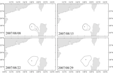
33 1
Figure 9. Evolution snapshots of ACE3’s merging event. The composite border is delineated 2
by the solid line while the footprint border is delineated by the dashed line. 3
4 5
Fig. 9. Evolution snapshots of ACE3’s merging event. The
compos-ite border is delineated by the solid line, while the footprint border is delineated by the dashed line.
shrinking eddy disappeared and the two-core structure even-tually turned into a single eddy. Such an evolution event of ACE3 recognized by HD is basically consistent with the de-scription in Nan et al. (2011). Additionally, the multi-core structure is delineated, providing detailed information (e.g., how the energy tranfers) about the merging effect.
The other long-lived anticyclonic eddy, i.e., ACE2, which split off a small eddy on 11 July according to Nan et al. (2011), is also examined, and Fig. 10 shows the identifica-tion results of HD during the split. On 4 July, ACE2 consti-tuted a two-core structure in a loose connection with ACE3, but one week later, they separated and ACE2 shrunk sig-nificantly. Afterwards, ACE2 was strengthened judging by the core areas, and contained in a more complex four-core structure on 18 July. In addition, between ACE2 and ACE3 a small newborn eddy can be observed expanding rapidly in the multi-core structure, which suggests that the evolution of ACE2 and ACE3 had contributed much to the generation and the development of this internal newborn eddy.
Some differences can be observed, relative to Nan et al. (2011), especially that ACE2 was not found splitting off a small eddy but rather separated from ACE3 during 4– 11 July. Careful examination reveals how this discrepancy results from the different detection criteria used. Nan et al. employed the OW method to identify eddies so that they ob-served the splitting event since ACE2’s core was indeed di-vided into two parts during that period. However, one part af-ter the separation contained no SLA local maximum and was consequently excluded from HD’s detection results. Despite some differences between the results of our algorithm and the description of Nan et al. (2011), our results demonstrate the feasibility of the automated detection even when eddy structures contain multiple cores, presenting a means to al-gorithmically identify splitting and merging events, enabling one to locate an entire class of events involving multiple eddy cores and a change in the number of eddies.
34 1
Figure 10. Evolution snapshots of ACE2’s splitting event. The dots represent eddy centers 2
while the dark grey polygons represent eddies’ core areas. The composite border is delineated 3
by the solid line while the footprint border is delineated by the dashed line. 4
5
Fig. 10. Evolution snapshots of ACE2’s splitting event. The dots
represent eddy centers, while the dark grey polygons represent eddy core areas. The composite border is delineated by the solid line, while the footprint border is delineated by the dashed line.
4 Conclusions
This study proposed a new hybrid method, HD, which is de-signed to automatically identify mesoscale eddies from SLA data sets. The combination of detection criteria of the OW method and the SSH-based method effectively enhances the accuracy of eddy detection, and procedures are implemented in the HD method to recognize the multi-core structure of mesoscale eddies, which serves as the foundation of track-ing eddies’ dynamic events (e.g., splitttrack-ing or mergtrack-ing) and eddies’ mutual interactions during the evolution processes.
To evaluate the detection accuracy of the HD method ob-jectively, this study adopted the validation protocol used by Chaigneau et al. (2008) and made a comparison with the manual results detected by 5 experts. Ten random experi-ments in the South China Sea showed that the average suc-cessful detection rate was ∼96.6 % and the excessive de-tection rate was∼14.2 %, which confirmed HD’s improve-ment in detection accuracy over either OW or the SLA extremum-based method individually. Second, the compar-isons between different detection algorithms in the ESP study area illustrated every method’s performance as well as HD’s capability of recognizing eddy multi-core structures. Finally, by comparing with two long-lived anticyclonic eddies inves-tigated by Nan et al. (2011), this study verified HD’s de-tection results and found that the merging event involving ACE3 was well recognized by HD, while the discrepancy of ACE2’s splitting event was mainly due to the different detec-tion criteria between OW and HD. This detecdetec-tion verificadetec-tion also demonstrated the additional capability of recognizing the multi-core structures, which facilitated the identification of the splitting and merging changes and unveiled details of eddy evolution that cannot be seen with other detection algo-rithms.
J. Yi et al.: Enhancing the accuracy of automatic eddy detection 47
sufficiently strong SLA. Although HD is able to address complex multi-eddy structures, the extent of mass or energy exchanges and interactions under the surface require further careful studies and validation with in situ data. So, having presented a method for the identification of multi-core struc-tures, we expect and welcome subsequent refinement to our method.
This study has developed a hybrid method for identifying single eddies and composite structures containing multiple cores from an instantaneous map of SLA. In the next pa-per, we will present the companion tracking method that is able to extract the continuous evolution processes as well as complex dynamic changes and interactions of the identified eddies and composite structures.
Acknowledgements. We thank Matthew Hecht, Sean Williams,
and other two anonymous reviewers for their constructive com-ments on this paper. We are grateful to Alexis Chaigneau for providing the detection results of their improved wind-angle method, and Francesco Nencioli for sharing the source code of the Vector-Geometry Eddy Detection Algorithm. We also thank the experts participating in the manual detection of eddies so that we can make method validations. This research was a contribution to research projects 41071250 and 41371378 of the National Science Foundation of China and 088RA500KA of the Innovation Projects of the State Key Laboratory of Resource and Environment Information System, Chinese Academy of Sciences. The altimeter products were produced by Ssalto/Duacs and distributed by Aviso, with support from Cnes (http://www.aviso.oceanobs.com/duacs/).
Edited by: M. Hecht
References
Ari Sadarjoen, I. and Post, F. H.: Detection, quantification, and tracking of vortices using streamline geometry, Comput. Graph., 24, 333–341, doi:10.1016/s0097-8493(00)00029-7, 2000. Basdevant, C. and Philipovitch, T.: On the validity of the “Weiss
criterion” in two-dimensional turbulence, Physica D, 73, 17–30, doi:10.1016/0167-2789(94)90222-4, 1994.
Chaigneau, A. and Pizarro, O.: Eddy characteristics in the eastern South Pacific, J. Geophys. Res., 110, C06005, doi:10.1029/2004jc002815, 2005.
Chaigneau, A., Gizolme, A., and Grados, C.: Mesoscale eddies off Peru in altimeter records: Identification algorithms and eddy spatio-temporal patterns, Prog. Oceanogr., 79, 106–119, doi:10.1016/j.pocean.2008.10.013, 2008.
Chelton, D. B. and Schlax, M. G.: The Accuracies of Smoothed Sea Surface Height Fields Constructed from Tandem Satellite Altimeter Datasets, J. Atmos. Ocean. Tech., 20, 1276–1302, doi:10.1175/1520-0426(2003)020<1276:taosss>2.0.co;2, 2003. Chelton, D. B., Schlax, M. G., Samelson, R. M., and de Szoeke, R.
A.: Global observations of large oceanic eddies, Geophys. Res. Lett., 34, L15606, doi:10.1029/2007gl030812, 2007.
Chelton, D. B., Schlax, M. G., and Samelson, R. M.: Global ob-servations of nonlinear mesoscale eddies, Prog. Oceanogr., 91, 167–216, doi:10.1016/j.pocean.2011.01.002, 2011.
Doglioli, A. M., Blanke, B., Speich, S., and Lapeyre, G.: Tracking coherent structures in a regional ocean model with wavelet anal-ysis: Application to Cape Basin eddies, J. Geophys. Res., 112, C05043, doi:10.1029/2006jc003952, 2007.
Dong, C., Liu, Y., Lumpkin, R., Lankhorst, M., Chen, D., McWilliams, J. C., and Guan, Y.: A Scheme to Identify Loops from Trajectories of Oceanic Surface Drifters: An Application in the Kuroshio Extension Region, J. Atmos. Ocean. Technol., 28, 1167–1176, doi:10.1175/jtech-d-10-05028.1, 2011.
Ducet, N., Le Traon, P. Y., and Reverdin, G.: Global high-resolution mapping of ocean circulation from TOPEX/Poseidon and ERS-1 and -2, J. Geophys. Res., 105, 19477–19498, doi:10.1029/2000jc900063, 2000.
Fang, F. and Morrow, R.: Evolution, movement and decay of warm-core Leeuwin Current eddies, Deep Sea Res.-Pt. II, 50, 2245– 2261, doi:10.1016/s0967-0645(03)00055-9, 2003.
Fawcett, T.: An introduction to ROC analysis, Pattern Recogn. Lett., 27, 861–874, doi:10.1016/j.patrec.2005.10.010, 2006.
Henson, S. A. and Thomas, A. C.: A census of oceanic anticyclonic eddies in the Gulf of Alaska, Deep Sea Res.-Pt I, 55, 163–176, doi:10.1016/j.dsr.2007.11.005, 2008.
Isern-Fontanet, J., Garcia-Ladona, E., and Font, J.: Identification of marine eddies from altimetric maps, 5, American Meteorological Society, Boston, MA, ETATS-UNIS, 7 pp., 2003a.
Isern-Fontanet, J., Garcia-Ladona, E., and Font, J.: Identi-fication of marine eddies from altimetric maps, J. At-mos. Ocean. Tech., 20, 772–778, doi:10.1175/1520-0426(2003)20<772:IOMEFA>2.0.CO;2, 2003b.
Isern-Fontanet, J., Garcia-Ladona, E., and Font, J.: Vortices of the Mediterranean Sea: An altimetric perspective, J. Phys. Oceanogr., 36, 87–103, doi:10.1175/JPO2826.1, 2006.
Jia, Y. and Liu, Q.: Eddy Shedding from the Kuroshio Bend at Luzon Strait, J. Oceanogr., 60, 1063–1069, doi:10.1007/s10872-005-0014-6, 2004.
Le Traon, P. Y. and Dibarboure, G.: Mesoscale Mapping Capabilities of Multiple-Satellite Altimeter Missions, J. Atmos. Ocean. Tech., 16, 1208–1223, doi:10.1175/1520-0426(1999)016<1208:MMCOMS>2.0.CO;2, 1999.
Li, L., Nowlin Jr., W. D., and Jilan, S.: Anticyclonic rings from the Kuroshio in the South China Sea, Deep Sea Res.-Pt. I, 45, 1469– 1482, doi:10.1016/s0967-0637(98)00026-0, 1998.
McWilliams, J. C.: the nature and consequence of oceanic eddies, in: Eddy-Resolving Ocean Modeling, edited by: Hecht, M. and Hasumi, H., AGU Monograph, 5–15, 2008.
Morrow, R., Birol, F., Griffin, D., and Sudre, J.: Divergent pathways of cyclonic and anti-cyclonic ocean eddies, Geophys. Res. Lett., 31, L24311, doi:10.1029/2004gl020974, 2004.
Nan, F., He, Z., Zhou, H., and Wang, D.: Three long-lived anticy-clonic eddies in the northern South China Sea, J. Geophys. Res., 116, C05002, doi:10.1029/2010jc006790, 2011.
Nencioli, F., Dong, C., Dickey, T., Washburn, L., and McWilliams, J. C.: A Vector Geometry–Based Eddy Detection Algorithm and Its Application to a High-Resolution Numerical Model Prod-uct and High-Frequency Radar Surface Velocities in the South-ern California Bight, J. Atmos. Ocean. Tech., 27, 564–579, doi:10.1175/2009jtecho725.1, 2010.
doi:10.1016/0011-7471(70)90059-8, 1970.
Pascual, A., Faugère, Y., Larnicol, G., and Le Traon, P.-Y.: Im-proved description of the ocean mesoscale variability by com-bining four satellite altimeters, Geophys. Res. Lett., 33, L02611, doi:10.1029/2005gl024633, 2006.
Penven, P., Echevin, V., Pasapera, J., Colas, F., and Tam, J.: Average circulation, seasonal cycle, and mesoscale dynamics of the Peru Current System: A modeling approach, J. Geophys. Res., 110, C10021, doi:10.1029/2005jc002945, 2005.
Petersen, M. R., Williams, S. J., Maltrud, M. E., Hecht, M. W., and Hamann, B.: A three-dimensional eddy census of a high-resolution global ocean simulation, J. Geophys. Res.-Oceans, 118, 1759–1774, doi:10.1002/jgrc.20155, 2013.
Robinson, S. K.: Coherent Motions in the Turbulent Bound-ary Layer, Annu. Rev. Fluid Mech., 23, 601–639, doi:10.1146/annurev.fl.23.010191.003125, 1991.
Wang, D., Xu, H., Lin, J., and Hu, J.: Anticyclonic eddies in the northeastern South China Sea during winter 2003/2004, J. Oceanogr., 64, 925–935, doi:10.1007/s10872-008-0076-3, 2008. Wang, G., Su, J., and Chu, P. C.: Mesoscale eddies in the South China Sea observed with altimeter data, Geophys. Res. Lett., 30, 2121, doi:10.1029/2003gl018532, 2003.
dipole in the South China Sea summer circulation, J. Geophys. Res., 111, C06002, doi:10.1029/2005jc003314, 2006.
Weiss, J.: The dynamics of enstrophy transfer in two-dimensional hydrodynamics, Physica D, 48, 273–294, doi:10.1016/0167-2789(91)90088-q, 1991.
Williams, S., Petersen, M., Bremer, P.-T., Hecht, M., Pascucci, V., Ahrens, J., Hlawitschka, M., and Hamann, B.: Adaptive extrac-tion and quantificaextrac-tion of geophysical vortices, IEEE T. Vis. Comput. Gr., 17, 2088–2095, 2011.
Xiu, P., Chai, F., Shi, L., Xue, H., and Chao, Y.: A census of eddy activities in the South China Sea during 1993–2007, J. Geophys. Res., 115, C03012, doi:10.1029/2009jc005657, 2010.
Yi, J., Du, Y., Wang, X., He, Z., and Zhou, C.: A clustering analysis of eddies’ spatial distribution in the South China Sea, Ocean Sci., 9, 171–182, doi:10.5194/os-9-171-2013, 2013.