Detecting Keratoconus by Using SVM and Decision Tree Classifiers with the Aid of Image Processing

Baghdad Science Journal

Vol.16 (4) Supplement 2019

DOI:http://dx.doi.org/10.21123/bsj.2019.16.4(Suppl.).1022

Detecting Keratoconus by Using SVM and Decision Tree Classifiers with the Aid

of Image Processing

Zahraa M. Mosa

Nebras H.Ghaeb

Alyaa H.Ali

Received 3/5/2018, Accepted 9/5/2019, Published 18/12/2019

This work is licensed under a Creative Commons Attribution 4.0 International License.

Abstract

:

Researchers used different methods such as image processing and machine learning techniques in addition to medical instruments such as Placido disc, Keratoscopy, Pentacam;to help diagnosing variety of diseases that affect the eye. Our paper aims to detect one of these diseases that affect the cornea, which is Keratoconus. This is done by using image processing techniques and pattern classification methods. Pentacam is the device that is used to detect the cornea’s health; it provides four maps that can distinguish the changes on the surface of the cornea which can be used for Keratoconus detection. In this study, sixteen features were extracted from the four refractive maps along with five readings from the Pentacam software. The classifiers utilized in our study are Support Vector Machine (SVM) and Decision Trees classification accuracy was achieved 90% and 87.5%, respectively of detecting Keratoconus corneas. The features were extracted by using the Matlab (R2011 and R 2017) and Orange canvas (Pythonw).

Key words: Decision Tree,Image processing, Keratoconus (KCN), Pentacam, SVM, Topographic Maps.

Introduction:

Keratoconus (KCN) is a bilateral non inflammatory disease that can be described as a thinning in the cornea and that will cause a cone like shape and a distortion in the vision(1). KCN is a progressive disease therefore it is important to diagnose the effected cornea at early stages to give the right treatment for it. Researchers put their efforts to improve the hardware as well as software to deliver devices that give accurate readings. There are different instruments to help in diagnosing Keratoconus(2); Pentacam is one of the most efficient devices that can gives readings as well as maps which gives indication of the corneas health(3). The maps that help to detect KCN are the four refractive maps; it consists of four maps (Sagittal, Pachymetry, Elevation front and Elevation back maps). All maps can be obtained individually and altogether in one image, each map gives numbers of factors; and after revising all of these factors that are extracted from the four refractive maps; the classifiers will make the final decision.

1 _{Department of Physics, College of Science for Women,}

University of Baghdad, Baghdad, Iraq.

2

Department of Biomedical Engineering, Al-Khawarzmi College of Engineering, University of Baghdad, Baghdad, Iraq.

*

Corresponding author: zahraaronan_1984@yahoo.com

Diagnosing KCN corneas faces certain difficulties; starting from observing the maps that are acquired from the Pentacam along with the reading and also utilizing the results of examinations from other instruments to give the final decision, all of this complicated process is to give an accurate decision to eventually have the right treatment.

In the current study, image processing, the geometrical calculations and pattern classifications methods will be utilized to classify the corneas whether it is a normal cornea or KCN affected cornea. Most of the previous studies did not extract features from the maps, as the extracted features from these maps can be considered as complementary to the readings obtained from the Pentacam software to detect KCN corneas. Therefore in our study features from the four refractive maps were extracted; these features along with few readings from the device were used as an input for the Support Vector Machine (SVM) and Decision Tree classifiers. The extracted details with the readings showed high accurate diagnosing; as a result this will help doctor decision.

Subjects and Data Collection:

Data set were acquired from Al-Amal Eye Private Clinic in Baghdad by using the Pentacam(OCULUS), where the cases were already examined and checked by a specialist doctor. The four refractive maps were used for this work to diagnose Keratoconus.

The data set of the 40 cases was consisted of 22 females and 18 males, divided into two groups 25 normal cases and 15 abnormal cases. In this study the corneal map for the right eye(OD)only from each case was used.

The work on the four refractive maps:

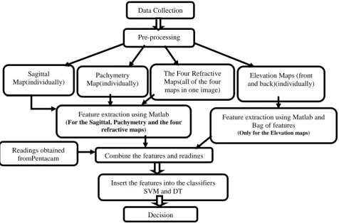
The work was divided into five stages depending on the features extracted from each map. All maps were converted from color maps into gray level, all features were extracted from 6 mm diameter circle and were applied to each map because most of the changes that indicate of having KCN will appear inside this area as it is the focal zone(9). Table 1 represents the features that have been extracted from the maps and the parameters (that have been taken from the Pentacam) that were taken as a reference. Figure 1 is represents the general idea of the work that was applied on the four refractive maps (Sagittal map, Pachymetry map, Elevation maps (front and back) and The Four Refractive map).

Figure 1. A block diagram of the general steps of the proposed work for KCN detecting Data Collection

Pre-processing

Elevation Maps (front and back)(individually) Pachymetry

Map(individually)

The Four Refractive Maps(all of the four maps in one image) Sagittal

Map(individually)

Readings obtained

fromPentacam Combine the features and readings

Feature extraction using Matlab and Bag of features

(Only for the Elevation maps) Feature extraction using Matlab

(For the Sagittal, Pachymetry and the four refractive maps)

Decision

Table 1.The four refractive maps and the extracted features

The Four Refractive Maps The Extracted Features The reading from the Pentacam

1- The Sagittal Map (individually)

1- The area of the bowtie parts. 2- The angle of skewing. 3- The mean of the K reading. 4- K2-K1

1-1K1 2- 2K2 3- K1 Axis

2- The Pachymetric Map (individually)

1- Determine the shape in the map (circle, ellipse, etc...).

2- Determine the center of the shape. 3- Determine the thinnest location.

1- The Thinnest Point Location

3- The Elevation Map Front(individually) 4-The Elevation Map Back (individually)

1- The angle of skewing. 2- The bag of features.

1-K1 2- K2 3- K1 Axis

5-The Four Refractive Maps (all maps togethr)

1- The thinnest points. 1- The Thinnest Point Location 2- The Thinnest Point Value

1

K1=The keratometry readings in the flat meridian, 2K2=The keratometry readings in the steep meridian

Extracting Features from Sagittal Map:

Three features that were extracted from this map are as explained in Table 1. After converting the map from RGB into gray level, a threshold was applied to separate the background from the

foreground shape(which is the bowtie shape that indicate of having astigmatism) and then splitting the shape from the middle into top half and bottom half to calculate the area of the shape as shown in Fig.2 (10).

(a) (b)

(c) (c)

Figure 2. In (a) the threshold to separate of the shape (bowtie) from the background and in (b) and(c)the splitting of the top and bottom halves of the shape.

If the area of both halves was nearly the

same then it could be said that it is within the G(x, y) = {

if the pixel = threshold then p = p + 1 if the pixel ≠ threshold then p = 0 .. 1 G(x, y)

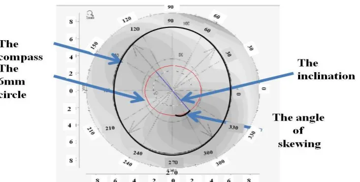
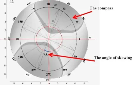
The other important feature that has been calculated from this map is the angle of skewing which is a very significant feature that gives another hint of the corneas health. The calculation of this angle is done by fitting the compass after doing pre-processing on it from converting it into grey level with 'jpg’ format to do the merging between the map and the compass. From knowing one of the axis which is K1 axis (provided from the Pentacam). The slope was calculated then from

knowing that the angle were calculated from eqs. 2 and 3 as showing in Fig.3.:

Slope =(x2-x1)/ (y2-y1) … 2

The angle = tan−1slope … 3

Where x1,x2,y1,y2 are the locations of the

two ends for the slope.

The angle is representing the skewing angle for the bowtie shape.

Figure 3. The compass fitting on the map and the slope to calculate the skewing angle (10)

The angle was converted from radian into degree as in eqs 4and 11.

Angle in degree = angle in radian *(180/pi)… 4 A comparison has been made between the angle of skewing and the subjective angle (which is an angle that acquired for the same patient from other devices). If the differences between the angles was less or equal to 10 degrees then according to ophthalmologist the cornea can be considered as within the normal range if not then it is a red flag (red flag is a term that will represent the results that are not within the normal values).

The other feature that has been calculated is the mean of the k readings it is done by using eq. 5and11:

K reading mean= (Kmean1+Kmean2)/2 … 5

Where: K mean1 is the mean value of two opposite Ks (K1+K2/2) in the flat meridian, and K mean2 is the mean value of two opposite Ks (K1+K2/2) in the steep meridian, the Ks can be obtained from the map.

If the K mean is close in value to K2 value then the cornea will be in the risk of having KCN and there will be a red flag, if it is closer in value to K1 value, then it is within the normal. Finally we also calculated the differences between K2 and K1 to know if the value is within the regular range or not, if the difference was within 1.5 dioptre then the cornea is normal, if it is not then there will be a red flag.

Extracting Features from Pachymetry Map:

Figure 4. Showing the contour that was applied on the Pachymetry map and the 6mm circle (in red color) also the horizontal and vertical meridians are shown to determine the horizontal and vertical diameter for the round line(10)

If the radius for both r1 and r2 are not equal,

then the joint line is ellipse and the cornea is within the normal range.If it is not, this means that it is circle and the cornea is in risk of having KCN and there will be a red flag.

r1 =│(x2- x1) │/ 2 …6

r2 =│ (y3- y4) │/ 2 …7

Where: r1 is the vertical radius.

r2 is the horizontal radius.

The other features that were determined from this map are the thinnest point and the center of the map as explained in Fig. 5.

Figure 5. Showing the thinnest point and the centre of the map for the Pachymetry map(10)

The location of the thinnest point has been taken from the device’s software and the center point location was determined from the map manually. A calculation of the distance between the two points has been made as in eqs. 8 and11, this distance (d) was compared with the horizontal and vertical diameters (2*r1,2*r2). If d is greater than

2*r1 and 2*r2 then this mean that one of the points

or both of them are outside the round line that within the 6mm diameter circle and the cornea is with the risk of having KCN, if not then it is

Where: d is the distance between the centre point and the thinnest location.

x1,x2,y1,y2 are the coordinates for the two points.

Extracting Features from Elevation Maps (Front and Back):

The work on these maps was divided into two parts depending on the techniques and the extracted features. The first extracted feature from Elevation maps (Front and Back) was the skewing angle, as the previous work on Sagittal map; after pre-processing these maps a compass was overlapped with them (after converting the compass from RGB to gray level and change the format into jpg). The angle of skewing was calculated from knowing the slope, and then this angle was compared with the angle of skewing for the Sagittal map for the same cornea and patient; if the angles were the same (which means the bowtie shape for both maps are in the same direction) then the cornea is ok, if they are not then it is red flag, as shown in Fig. 6.

Figure 6. The compass fitting on Elevation maps front and back

Extracting Features from the Four Refractive Maps:

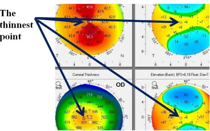
A single image which has all the four refractive maps was used as shown in Fig.7. The feature extracted from these maps was the thinnest point location. As the Pentacam software gives the location and value of the thinnest point for the

Pachymetry map; the thinnest point location was determined for the rest of the maps as shown in Fig.8; and the value of them was compared. If the values for the thinnest points were within the normal range that the ophthalmologist agreed on, then the cornea is ok.Ifit is not, then there will be a red flag.

Figure 7.Showing the Four Refractive Maps together in one image

Figure 8. The thinnest point for the Four Refractive Maps(10)

The Classifiers:

After extracting the features form all of the 40 cases, SVM and Decision Tree classifiers were applied on the cases to know the final diagnosing. SVM is one of the most recently used methods. Its basic work is to separate data in the most optimal method by finding a hyper-plane to do so, as a result it will give the final decision (13- 15). Decision Tree(DT) classifier is another method of classification that is used to make decisions and also

and DT classifier we used only SVM and DT classifiers in the final results.

Classifiers were applied on the extracted features to give the final decision. After trying different range of settings to find the optimal result for both classifiers; linear SVM was used with Cost (C) of 0.30 and regression loss epsilon (ε) of 1.00, where the setting for the Decision Tree for the minimal number of instance in leaves was 7. These settings were the best settings that gave the highest accuracy, and to maximize the accuracy for the final decisions; the leave one out cross validation method was used to make sure that each case will be tested and compared with the other cases. Eq. 9. (20) was used to compute the accuracy for our used classifiers

𝐴𝑐𝑐𝑢𝑟𝑎𝑐𝑦 =_{𝑇𝑜𝑡𝑎𝑙𝐶𝑎𝑠𝑒𝑠}𝑇𝑃+𝑇𝑁

𝑁𝑜.

100% … 9

Where TP is the true positive and TN is the true negative.

Results and Discussion:

Diagnosing Keratoconus disease can be a confusing process, especially at early stages, so in order to give an accurate diagnosing there should be more factors examined for the cornea before the final decision is made. Therefore in this study we focused on extracting features from the maps itself as well as using some readings from the software of the Pentacam as a guide for the extracted features to support the doctor point of view.

The confusion matrices(21)in Tables 2 and 3, show the match and mismatch cases for each class between doctors decision and each classifiers for the 40 cases, for the SVM and Decision Tree classifiers respectively.

Table 2. The confusion matrix for the SVM classifier Do ct or’ s decisi o n SVM

KCN NORMAL ∑sum

KCN 12

(TP)

3 (FN)1

15

NORMAL 1

(FP)2

24 (TN)

25

∑sum 13 27 40

FN1 is the false negative,FP2 is the false positive

Table 3. The confusion matrix for the Decision Tree classifier or’ s o n Decision Tree

KCN NORMAL ∑sum

KCN 11 4 15

FN1 is the false negative,FP2 is the false positive

The overall accuracy, calculated from eq. 9 for the 40 cases of the SVM and Decision Tree classifiers were 90% and 87.5% respectively. It appears that the SVM is more accurate in diagnosing than the Decision Tree classifier. Both classifiers showed high percentage in detecting the KCN and normal cases and low percentage for the wrong mismatch cases. Most of the cases matched doctors’ diagnosis and the maximum and minimum values were taken from the ophthalmologist’s values, in some cases the readings that have been taken from the Pentacam were within normal values but the maps showed many abnormal signs that indicates that the cornea is affected with KCN.

Conclusion:

Our system is found to be as a supportive system to doctors’diagnosis. After reviewing the results from classifiers of each case and match those results with the doctor’s diagnosis, the final decision will be made. If the classifiers prediction will match the doctor’s diagnosis; then the treatment will proceed to the patient that suffers from KCN, if the results for the classifiers will not match doctor’s decision; then the doctor will be advised to make further examination before giving the final diagnoses. A detection accuracy of 90% and 87.5% was obtained with the proposed system when utilizing our extracted features and SVM and DT classifiers. This may help the doctor for a better diagnose of KCN cases.

Conflicts of Interest: None.

Reference:

1. Castillo J H, Hanna R, Berkowitz E, Tiosano B. Wavefront Analysis for Keratoconus.Int J Keratoconus Ectatic Corneal Dis.2014;3(2): 76–83. 2. Cavas-Martínez F, De la Cruz Sánchez E, Nieto

Martínez J, Fernández Cañavate F J, Fernández-Pacheco D G. Corneal topography in keratoconus: state of the art.Eye Vis. 2016 Jan; 3(5):1–12.

3. Abu Ameerh M A, Bussières N, Hamad G I, Al Bdour M D. Topographic characteristics of keratoconus among a sample of Jordanian patients. Int J Ophthalmol 2014 Jan; 7(3):714–19.

4. Accardo P A, Pensiero S. Neural network-based system for early keratoconus detection from corneal topography.J Biomed Inform.2003;35(2003):151– 159.

Machine Learning for Health-Care Applications.2008.

7. Twa M D, Parthasarathy S, Raasch T W, Bullimore M A. Decision Tree Classification of Spatial Data Patterns From Videokeratography Using Zernike Polynomials. SIAM International Conference on Data Mining. 2003;3–12.

8. Toutounchian F, Shanbehzadeh J, Khanlari M, Stage A R. Detection of Keratoconus and Suspect Keratoconus by Machine Vision. Int. M. J Comput Sci.2012; I: 14–16.

9. Association American Academy of ophthalmology the eye M D, Fundamentals and principles of ophthalmology. 2016; 2:66 – 71.

10. Ali A H, Ghaeb N H, Musa Z M. Support Vector Machine for Keratoconus Detection by Using Topographic Maps with the Help of Image Processing Techniques.J Pharm Biol ci.2017;12(6):50–58. 11. George J, Thomas B. Thomas’ Calculus Early

Transcendentals,13ed. USA: Pearson Education; 2014: p.299–390.

12. Barata C, Ruela M, Mendonça T, Marques J S. A Bag-of-Features Approach for the Classification of Melanomas in Dermoscopy Images : The Role of Color and Texture Descriptors. Series in Bio Engineering Eds. Berlin: Springer-Verlag Berlin Heidelberg.2014:.49–69.

13. Demidova L.The SVM Classifier Based on the Modified Particle Swarm Optimization.Int J Adv Comput Sci Appl.2016;7(2):16–24.

14. Yekkehkhany B, Safari A, Homayouni S, Hasanlou M. A Comparison Study of Different Kernel Functions for SVM-based Classification of Multi-temporal Polarimetry SAR Data Int Arch

Photogramm Remote Sens Spat Inf

Sci.2014;XL(2/W3):15–17.

15. Assen D, Akour S, Aleb H T. A Hybrid Fuzzy-SVM classifier for automated lung diseases diagnosis. J Med Phys Eng.2016; 22(4): 97–103.

16. Dai W, Ji W.A Map Reduce Implementation of C4.5 Decision Tree Algorithm.Int J Database Theory Appl.2014;7(1): 49–60.

17. Sharma H, Kumar S. A Survey on Decision Tree Algorithms of Classification in Data Mining.Int J Sci Res.2016;5(4):2094–2097.

18. Badr A, Din E, Elaraby I S. Data Mining : A prediction for Student ’ s Performance Using Classification Method. World J Comput Appl Technol.2014;2(2):43–47.

19. Kotsiantis S B, Zaharakis I D, Pintelas P E.Machine learning : a review of classification and combining techniques.Springer Sci Media.2007; 26( 2006):159– 190.

20. Lalkhen AG, McCluskey A. Clinical tests: sensitivity and specificity. Continuing Education in Anaesthesia Critical Care & Pain. 2008 Dec 1;8(6):221-3.

21. Santra A K,Christy C J.Genetic Algorithm and Confusion Matrix for Document Clustering . Int J Comput Sci.2012;9(1):322–328.

فينصتلا اتقيرط مادختساب ةيطورخملا ةينرقلا ضرم صيخشت

روصلا ةجلاعم قرط و

Decision Tree

و

SVM

ىسوم كلام ءارهز

بئاغ نيسح ساربن

يلع نيسح ءايلع

1

لا ةيلك ،ءايزيفلا مسق دادغب ،دادغب هعماج ،تانبلل مولع

.قارعلا ،

2

طلا ةسدنه مسق يمزراوخلا ةسدنه ةيلك ،يتايحلا ب

دادغب ةعماج ، .قارعلا ،

ةصلاخلا

:

قرط و روصلا ةجلاعم تاينقت مادختساب كلذ مت و ةيطورخملا ةينرقلا يهو ،ةينرقلا بيصت يتلا ضارملاا نم عون ديدحت وه انثحب فده اكاتنبلا زاهج . فينصتلا تاريغت نع فشكت يتلاو طئارخ يطعي زاهج نع ةرابع وه يذلاو ةينرقلا ةحص صيخشتل مدختسملا زاهجلا وه م

رشع ةتس تجرختسا انثحب يف . ةيطورخملا ةينرقلا ضرم صيخشتلو فشكلل همدختسملا طئارخلا يه ةعبرلاا ةيراسكنلاا طئارخلا و ةينرقلا لااب ةعبرلاا ةيراسكنلاا طئارخلا نم ةصيصخ جئاتن قينصتلا يتقيرط جئاتن ترهظا دقو .ماكاتنبلا زاهج نم ةذوخأم تاءارق سمخ ىلا ةفاض

بسنب هديج 87,5

و 90 .ةيطورخملا ةينرقلا صيخشتل يلاوتلا ىلع ةئملاب SVM

و Decision Tree

:ةيحاتفملا تاملكلا

. DECISION TREE,SVM رخلا ، ماكاتنبلا ،ةيطورخملا ةينرقلا،روصلا ةجلاعم