© Author(s) 2009. This work is distributed under
the Creative Commons Attribution 3.0 License.
in Geophysics
Quantitative analysis of randomness exhibited by river channels
using chaos game technique: Mississippi, Amazon, Sava and
Danube case studies
G. ˇZibret1and T. Verbovˇsek2
1Geological Survey of Slovenia, Ljubljana, Slovenia
2University of Ljubljana, Faculty of Natural Sciences and Engineering, Department of Geology, Ljubljana, Slovenia
Received: 23 October 2008 – Revised: 23 March 2009 – Accepted: 28 May 2009 – Published: 23 June 2009
Abstract. This paper presents a numerical evaluation of the randomness which can be observed in the geometry of major river channels. The method used is based upon that of gen-erating a Sierpinski triangle via the chaos game technique, played with the sequence representing the river topography. The property of the Sierpinski triangle is that it can be con-structed only by playing a chaos game with random values. Periodic or chaotic sequences always produce an incomplete triangle. The quantitative data about the scale of the ran-dom behaviour of the river channel pathway was evaluated by determination of the completeness of the triangle, gener-ated on the basis of sequences representing the river channel, and measured by its fractal dimension. The results show that the most random behaviour is observed for the Danube River when sampled every 715 m. By comparing the maximum di-mension of the obtained Sierpinski triangle with the gradient of the river we can see a strong correlation between a higher gradient corresponding to lower random behaviour. Another connection can be seen when comparing the length of the segment where the river shows the most random flow with the total length of the river. The shorter the river, the denser the sampling rate of observations has to be in order to obtain a maximum degree of randomness. From the comparison of natural rivers with the computer-generated pathways the most similar results have been produced by a complex super-position of different sine waves. By adding a small amount of noise to this function, the fractal dimensions of the gener-ated complex curves are the most similar to the natural ones, but the general shape of the natural curve is more similar to the generated complex one without the noise.
Correspondence to: G. ˇZibret ([email protected])
1 Introduction
not strictly self-similar objects, but rather self-affine (Beau-vais and Montgomery, 1997) and thus, empirically derived dimensions for these objects are only estimates of their true fractal dimension. The ideal surface with a fully developed river network should have a fractal dimension of 2, implying topological randomness. However, geological, topological and hydrological effects dictate that the fractal dimension of networks are always lower than 2 (La Barbera and Rosso, 1989). There are not many studies concerning individual river channels, as most studies have focused on drainage pat-terns (Tarboton et al., 1988; Nikora et al., 1993; Schuller et al., 2001; Angeles et al., 2004; De Bartolo et al., 2006 and others). The multifractal method has also been used for description of multichannel rivers (Veneziano and Niemann, 2000; De Bartolo et al., 2000; Gaudio et al., 2006 and oth-ers).
In this paper a novel approach has been used for the quan-titative analysis of the behaviour of the river channel from its source to its mouth. It is based on creating a Sierpin-ski triangle (also known as SierpinSierpin-ski gasket) via the chaos game, based on the data of the geometry of the channel. The chaos game is a method of generating deterministic ob-jects from apparently random ones (Barsnley, 1988; Peitgen et al., 2004). It can be used to produce a visual represen-tation of a sequence of random numbers (Mata-Toledo and Willis, 1997). It has been usefully applied to studies of DNA sequences (Jeffrey, 1992) and economics (Matsushita et al., 2007). The complete Sierpinski triangle via chaos game can be produced only with the help of the “perfect dice”, i.e. by an entirely random process. Every periodic sequence fails to reproduce a complete triangle and only some parts of it are created.
This paper presents an application of the chaos game al-gorithm to the characterisation of the randomness of river channel geometry. This approach concerns neither the frac-tal analysis of a single river channel nor the fracfrac-tal analysis of river networks, as both have been already studied exten-sively by many other authors (see paragraph above). Here, the river is analysed on the basis of the representation of its pathway with the sequence of three classes which act as an input for the chaos game. Following this the fractal dimen-sion of the outcome of the chaos game (a more or less com-plete Sierpinski triangle) is the measure of the randomness of the sequence representing the randomness of the river chan-nel. When the river forms perfect meanders or when it flows straight, the obtained sequence would be very deterministic and only a limited part of the Sierpinski triangle would be created. Hypothetically when the river behaves completely unpredictably, as the perfect dice do, the sequence will be random and a complete triangle should appear. All interme-diate possibilities produce more or less incomplete triangles. The higher the randomness of the river geometry, the higher the dimension of the triangle will be. Another issue to be mentioned is the sampling rate, which describes the length of the sequence which represents the river pathway. The denser
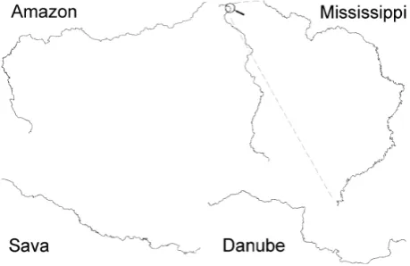
Fig. 1. Analysed rivers (scale varies, projection to Euclidean plane).
the sampling rate, the longer the sequence and the shorter the segment between two sequence points and vice versa.
2 Materials and methods
2.1 The choice of rivers and sources of data
Four rivers were analysed in this study – the Amazon, Missis-sippi, Danube and Sava (the largest tributary of the Danube) (Fig. 1). These watercourses were selected as their maps are easily accessible and they belong to different geologic and climatic environments. The river courses were digitised from various sources. The Amazon was digitised from the data on the Microsoft Encarta World Atlas web site1; the Mississippi from the Google Earth web site2; the Danube from the topographic maps on a scale of 1:200 000 from the 3rd Military Mapping Survey of Austria-Hungary (between the years 1889–1915)3; and the Sava from the national maps of former Yugoslavia on a scale of 1:25 000 (raster TIF im-ages). Despite the fact that we have used maps of different scales, all of them were sufficiently precise to present all of the river meanders and other necessary details. Moreover, different map scale does not affect the results because rivers were later in the process split into the 3-class sequence and this process is not affected by the map scale. Additionally, all of the rivers are very large so all of them were projected to the Euclidean plane. This had to be done as on the Eu-clidean plane all the geometrical calculations and manipula-tions are much easier to perform and such a projection should not much affect the obtained dimension of the Sierpinski tri-angle because the sequencing was done before the tritri-angle was constructed. Chaos game technique is also not very sen-sitive to errors because of the iterative nature of the process, so the results quickly stabilise after approximately 10 steps.
1http://encarta.msn.com/map 701510067/Amazon (river).html
2http://earth.google.com/
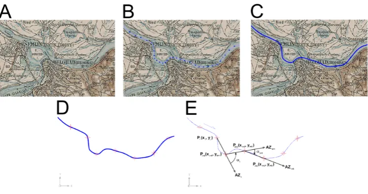
Fig. 2. The procedure for converting the river topography into a set of angles. (A) – raw tiff map; (B) – digitalisation using polyline method; (C) – conversion of the polyline into spline; (D) – division of spline into a defined set of segments – points (1000-segment Danube case); (E)
– calculation of the set of angles.
Prior to sequencing, the rivers were digitised using a com-mercial software AutoCAD package (Autodesk, Inc.) with a single polyline which was later transformed to spline which better represents the course of water flow. In cases where the river behaves as a “braided river” (has several active channels) only the most active channel was digitised due to the limitations of our methodology. Although braided rivers can be analysed using special techniques (Sapozhnikov and Foufoula-Georgiou, 1996), the chaos game algorithm re-quires that the rivers are presented with only one channel, digitised as a continuous line (spline). Similarly, the path-ways through the lakes were digitised as a spline (as a single channel) fitting from feeder to effluent locations.
Another issue has to be discussed prior to the generation of the sequence. Digitalisation started at the river mouth, go-ing upstream. Accordgo-ing to the Horton-Stahler stream order-ing system, the longest lower-ordered channel was proceeded along.
2.2 Generation of a direction sequence
The main difficulty of this research was the transformation of the topography of the river channel into the three differ-ent classes needed to “play” the chaos game. The proce-dure was as follows. The river courses were digitised from the image files (Fig. 2A) using Autodesk AutoCAD soft-ware with the polyline method (Fig. 2B). The polylines were then smoothed into splines (Fig. 2C), to simulate the natural course as much as possible. A fixed number of points were drawn along the curves for each analysis. Their quantities were chosen exponentially, as a power of 2: 1000, 2000, 4000, 8000, 16 000 and 32 000 (Fig. 2D) and will be
de-scribed by the terms “sampling rate” or “segment length” in this article. The lower limit of 1000 points was regarded as the minimum requirement for a Sierpinski triangle image analysis. Raising the number of points above 32 000 was not reasonable because it would yield very monotonous se-quences of classes. As a result, 24 arrays of points Pi with
coordinates (xi, yi)were obtained for further calculations,
where imaxvaries from 1000 up to 32 000 (Fig. 2E). The
fi-nal step of this procedure was to calculate the array of the angles (αi, Fig. 2E) which describe the topography of the
river by using Eq. (1) and Eq. (2). Following this procedure, the two azimuths from the first point, Pi−1(xi−1, yi−1,)to the
second one Pi(xi, yi), and from the second point to the third
one Pi+1(xi+1, yi+1,)have to be calculated by Eq. (1). That
is how the two azimuths AZiand AZi+1have been obtained.
The second step is the calculation of the angles (αi)between
these two azimuths using Eq. (2). The number of obtained angles is therefore equal to the number of points minus two.
AZi=
(xi+1−xi) >0⇒AZi=90◦−180
◦
π ·arctan y
i+1−yi xi+1−xi
(xi+1−xi) <0⇒AZi=270◦−180
◦
π ·arctan
yi+1−yi xi+1−xi
xi+1=xi⇒AZi=
(yi+1−yi) <0⇒AZi=180◦ (yi+1−yi) >0⇒AZi=0◦
(1)
αi=
(AZi+1−AZi) <−180◦⇒αi=(AZi+1−AZi)+360◦ (AZi+1−AZi) >180◦⇒αi=(AZi+1−AZi)−360◦
−180◦≤(AZ
i+1−AZi)≤180◦⇒αi=AZi+1−AZi
(2)
Finally, the array of the angles was classified into the three classes. If the direction was inclined to the left more than the critical angleαL., the segment was assigned a value ofL.
A value ofR was assigned if the direction to the right was greater than a critical angleαR and the valueF (forward)
Fig. 3. Technique testing results for various pseudo-random and
non-random generators: (A) – digits ofπ, (B) – digits of e, (C) – MS Excel RAND() function, (D) – LCG algorithm, (E) – bifurca-tion equabifurca-tion, (F) – sinus funcbifurca-tion. In cases D and F the size of the points has been enhanced due to visibility and in cases E and F the borders of the triangle have been included for easier visibility.
0,95 1 1,05 1,1 1,15 1,2
1000 10000 Number of segments 100000
F
ra
c
ta
l
d
im
e
n
s
io
n
o
f
th
e
S
ie
rp
in
s
k
i
tr
ia
n
g
le
(
D
)
Mississippi Sava Danube Amazon
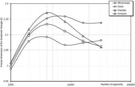
Fig. 4. The dimensions of the Sierpinski triangle, obtained via the
chaos game procedure in relation to the number of segments.
The angles were determined by the percentiles of 33.33% and 66.67% of the complete array of angle deviation, to keep the directions uniformly distributed in all three classes and also to avoid the impact of angle choice on the results. For instance, with large critical angles, most of the directions would fall into the F group, and contrarily, with low criti-cal angles, great deviations (mostly L and R) would appear. This was done to obtain the most complete triangle possible. A sequence with dominant L and R classes will yield a trian-gle with points concentrated only on one side of the triantrian-gle. On the other hand, a sequence with the F class dominant will result in a triangle with concentration of points close to the one corner. Finally, a sequence of letters was assigned to the river channel pathway, for instance LLRRRFFLRFLLL-RFRL, which was used as the input for the chaos game.
Fig. 5. Plot of chaos game results for the Amazon River, divided
by different numbers of observations. (A) – 1000, (B) – 2000, (C) – 4000, (D) – 8000, (E) – 16 000 and (F) – 32 000 observations. Lower left vertex attracts flow directions to the left (L), lower right forward (F) and upper vertex directions to the right (R).
2.3 The analysis of chaotic behaviour by the chaos game technique
The sequences were analysed by the method of the chaos game (Barnsley 1988; Jeffrey, 1992; Peitgen et al., 2004). This technique is useful for the determination of random pat-terns in data. The original method relies on visual estima-tion and in this paper it has been updated to a quantitative approach by examining the fractal dimensions of different approximations of Sierpinski triangles. The “game”, played long enough with a random sequence, produces a complete Sierpinski triangle (Mandelbrot, 1983). If a non-random gen-erating sequence is used, the Sierpinski triangle does not completely appear, as in the case of pseudo-random number generators with short periods, logistic equations or periodic functions (Figs. 3D, E and F). If the random numbers are not properly balanced (for example if some weight is placed on the one side of the dice), the triangle appears biased towards one vertex with greater probability.
The chaos game technique is described in detail in many references (Jeffrey, 1992; Mata-Toledo and Willis, 1997; Peitgen et al., 2004 etc.), so only a brief description is pre-sented here. Points in the equilateral triangle are drawn by the iteration technique with a simple rule: one class is as-signed to every corner of the triangle and the seed point is chosen randomly. The next point is drawn halfway between the previous point and the corner of the triangle, correspond-ing to the class in the sequence. In all cases in this research the seed point of the triangle has been chosen at the origin of the Euclidean coordinate system P0(0, 0).
Table 1. Results for testing the technique with random and
non-random number generators. D – fractal dimension of the con-structed triangle; R2 – correlation between dots on the log-log plot and the linear regression interpolation;dif% – difference be-tween Sierpinski triangle mathematical dimension andD in per-cent. The mathematical dimension of the Sierpinski triangle is D=log(3)/log(2)∼=1.585.
Generator D R2 dif%
pi 1.5567 0.9965 1.78
e 1.5563 0.9964 1.78
RAND() 1.5518 0.9963 1.78
LCG 1.0108 0.8796 36.2
bifurcation 1.0226 0.9807 35.5
sinus 0.4728 0.8125 75
chaos game, theoretically 1.5850 1 0 played with “perfect dice”
literature is stated that 10 000 points are needed to construct a Sierpinski triangle (Peitgen et al., 2004). The sequences are:
– Digits of the constantπ. The digits were grouped into packets of 8 decimals and divided by 108. Thus, a num-ber in the range of 0 to 1 was obtained. By the rules of the chaos game, the numbers were classified into three equal sized groups, each corresponding to the triangle vertices. A similar approach was applied to the follow-ing formulas.
– Digits of the constante, grouped into 10 digits. – Bifurcation equation. The sequence was obtained by
the iterated equation: a(n+1) = 3.999·a(n)·(1 - a(n)) (Peitgen et al., 2004) with the value a1between 0 and 1.
This sequence exhibits chaotic behaviour as its period is infinite or nearly infinite and the sequence is very sensi-tive to the initial conditions.
– LCG: linear congruential generator generates pseudo-random sequences and has a general equation of the form f(x+1) = (a · f(x) + n) (mod m) (Mata-Toledo and Willis, 1997). It requires three parameters (a, n and m), and in this study the formula a(n + 1)= (600·a(n)+500) (mod 977) with the number 5 as a seed has been used. Using this array of parameters the func-tion is periodical with a period of 976 iterafunc-tions. – RAND() random generator, as an internal function in
MS Excel application. This generator is supposed to be superior to other pseudo-random number generators and
0,4 0,6 0,8 1 1,2 1,4
1000 10000 no. of segments 100000
F
ra
c
ta
l
d
im
e
n
s
io
n
o
f
th
e
S
ie
rp
in
s
k
i
tr
ia
n
g
le
(
D
)
supersin complex sinus rivers internal noise external noise
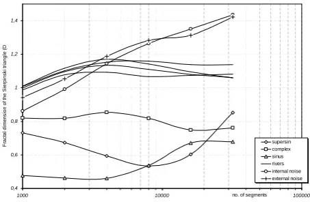
Fig. 6. The comparison of fractal dimensions of natural rivers and
the artificially computer-generated curves.
is guaranteed not to repeat the sequence until the value of 1013iterations (MS Excel help).
– Sinus function:a(n)=sin(n); n∈N where n is expressed in radians to avoid periodical sampling of the sinus function.
2.4 Determination of the fractal dimension of obtained Sierpinski triangles by box-counting method The fractal dimensions of the Sierpinski triangles were de-termined by the box-counting method, which has the most applications in science (Peitgen et al., 2004) and is probably also the most commonly used, as the principle of its use is rather simple. The digitised map of an object (for instance, a river or fracture network) is covered by boxes of differ-ent side lengthss, and then the number of occupied boxes N (s)is counted for each box size (Feder, 1988; Bonnet et al., 2001). The process is repeated by reducing the box sizes until the minimum size is reached. For fractal objects, the number of occupied boxesN (s)follows the power-law rela-tionship with the box sizesEq. (3).
N (s)≈s−D (3)
The fractal dimensionDis therefore calculated as the slope of linear regression best-fit line of log–log data, Eq. (4) (Foroutan-pour et al., 1999).
D= −logN (s)/logs (4)
The coefficient of determinationR2represents the value of how closely the linear regression fits to the plotted log-log data.
Sava Amazon Danube Mississippi 1,08 1,1 1,12 1,14 1,16 1,18
0 0,2 0,4 0,6 0,8 1 1,2 1,4 Average gradient of the river (m/km)
M a x . d im e n s io n o f th e t ri a n g le
Fig. 7. Scaling between average gradient of the river, expressed in
metres per kilometre with the maximum dimension of the triangle, acquired via the chaos game.
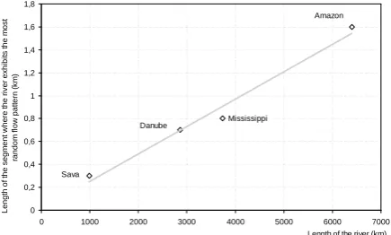
Amazon Mississippi Danube Sava 0 0,2 0,4 0,6 0,8 1 1,2 1,4 1,6 1,8
0 1000 2000 3000 4000 5000 6000 7000 Length of the river (km)
L e n g th o f th e s e g m e n t w h e re t h e r iv e r e x h ib it s t h e m o s t ra n d o m f lo w p a tt e rn ( k m )
Fig. 8. Length of the segment where the river expresses the most
random behaviour in relation to its total length.
dimensions. In this way, the generated image of the tri-angle was quantified and subjective visual judgments were avoided. All of the triangles were drawn as 1024×1024 black and white bitmap images prior to the box counting procedure. This resolution provides a satisfactory compromise between the resolution of the image and the number of pixels. 2.5 Computer generated lines
In order to evaluate our results, the same procedure was ap-plied to three different mathematical functions which might represent the natural rivers. Since the angles are not pre-served when the stretching of channel geometry in any of co-ordinate axes is performed, the precise functions will be pre-sented. First one is a simple sinus function (Eq. 5). The sec-ond one, named as “supersin” is a superposition of four sine waves (Eq. 6) with different amplitudes and wavelengths. In all cases empirical coefficients are chosen in such way that the functions behave similarly to the natural rivers.
sinus 500x = sin 100x
x=1...32 000rad (5)
supersin2π x360=0.7·sin(x/50)+sin(x/100) +1.4·sin(x/250)+2·sin(x/1000)
x=1...30 000rad
(6)
The third function is a complex superposition of sine waves named “complex” (Eq. 7) where we tried to simulate the nat-ural flow of the river as accurately as possible.
complex2π x360=5·sin(0.5x)+0.1·e(x−150)
2
5000 ·sin(7x)
+x·360·sin(0.1x)
2·π·1000 +10·sin(3
√ x)
x=1...30 000rad
(7)
A complex function is made from four waves (in the same order as in the Eq. 7):
– a basic wave with constant wavelength and amplitude; – a high frequency wave with a changing amplitude
de-scribed by a gaussian function, which is set to be maxi-mum in the first third, resembling small meanders in the upper flow of the river;
– a low frequency wave with an increasing amplitude to resemble long-wavelength meanders at the lower flow of the river;
– a steady amplitude but an increasing frequency wave to simulate flow without meanders, conditioned by the re-gional tectonic conditions in the upper part of the rivers. Finally we added a low amount of noise to the complex func-tion. Two different approaches have been used. Internal noise approach means that the noise has been added to the dependent variable and external noise approach means that the noise has been added to the functional result (Eq. 8). In both cases noise influenced approximately 1% of the fluctu-ations.
internal(x)=complex(x+noise)
external(x)=complex(x)+noise (8)
External noise can be explained geologically by the influ-ence of external geological factors, such as geomorphology or tectonic control on a greater observation scale, with pos-sible major faults dictating the directions and deviations of the river course while internal noise is explained by devia-tions inside the river channels, and these are obviously less important than the external deviations.
3 Results
3.1 Results of testing of the method used in the research
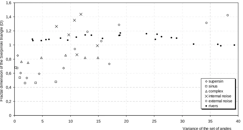
0 0,2 0,4 0,6 0,8 1 1,2 1,4 1,6
0 5 10 15 20 25 30 35 40
Variance of the set of angles supersin sinus complex internal noise external noise rivers
F
ra
c
ta
l
d
im
e
n
s
io
n
o
f
th
e
S
ie
rp
in
s
k
i
tr
ia
n
g
le
(
D
)
Fig. 9. The dimension of the triangle in relation to the variability of the angles.
Table 2. Results for the four analysed rivers. N – number of segments; AA – average angle (degrees); SD – standard deviation of the angles;
D – fractal dimension of the “triangle”;R2– coefficient of determination.
Amazon River Danube River
N AA SD D R2 N AA SD D R2
1000 −0.073 39.35 0.9981 0.8901 1000 −0.090 32.07 1.0108 0.8891
2000 −0.017 28.99 1.0974 0.9243 2000 −0.049 26.32 1.1172 0.9231
4000 −0.004 18.73 1.1338 0.9399 4000 −0.029 18.95 1.1705 0.9453
8000 −0.001 11.10 1.1110 0.9459 8000 −0.016 12.68 1.1421 0.9480
16000 −0.001 6.20 1.0796 0.9423 16000 −0.008 8.25 1.0953 0.9476
32 000 0.000 3.30 1.0615 0.9453 32 000 −0.002 4.81 1.0598 0.9499
Mississippi River Sava River
N AA SD D R2 N AA SD D R2
1000 −0.230 36.40 1.0076 0.8951 1000 0.019 36.93 0.9881 0.8846
2000 −0.134 28.06 1.1031 0.9225 2000 0.003 25.20 1.0784 0.9177
4000 −0.054 25.52 1.1525 0.9512 4000 0.002 15.76 1.0925 0.936
8000 −0.031 23.63 1.1585 0.9477 8000 −0.003 9.52 1.0666 0.9314
16000 −0.015 18.25 1.1383 0.9503 16000 −0.001 5.65 1.0735 0.94
32 000 −0.007 13.76 1.1379 0.9552 32 000 0.000 3.24 1.0815 0.9462
digits and the RAND() function is satisfactory as the Sier-pinski triangle was drawn accurately (Fig. 3A, B and C) and the obtained dimension is the greatest. The small difference between the dimensions of the triangle generated by decimal
chaotic sequences, are presented in Fig. 3D, E and F where the triangle was incomplete or even indistinguishable. The conclusion is that the methods used for creating the trian-gle and calculating its fractal dimension are acceptable and that the systematic error encountered in using this specific methodology is less than 2%.
3.2 Chaos game representation of the analysed rivers Since it has been established that the methodology yields ac-curate results, the sequence from the river directions was used to construct the Sierpinski triangle. As a result, the calculated dimension was used as a measure of how much a river channel flows randomly in its course. The more ran-domness it contains or, in other words, the more non-periodic behaviour it exhibits, the more faithfully the complete trian-gle is reproduced and the larger is the dimensionD. Table 2 shows the results and also basic statistical parameters of the set of angles prior to 3-class transformation, while Fig. 4 rep-resents the results graphically.
3.2.1 The Amazon
Obtained triangles for the Amazon River sequence are pre-sented in Fig. 5. The largest dimension of the triangle is for a segment length of 4000 points (Table 2, Fig. 4), as the trian-gle was reproduced most closely in this case (Fig. 5C). With a total length of approximately 6400 km, this means that the Amazon River exhibits the greatest random behaviour at a sampling rate of every 1.6 km. For the largest amount of data (32 000), the points in the triangle are drawn mostly on its edges.
As the segment length increases (or number of points de-creases), it is expected that the random behaviour is less pro-nounced on this scale, because the river channel topography on a large scales follows the macrotectonic environment and regional geological structures and is not very sensitive to lo-cal conditions, as is seen in denser observations. In addition, the meanders cannot be seen at this sampling rate. The re-sults clearly confirm these expectations.
3.2.2 The Mississippi
Similar results were obtained for the Mississippi River, and the dimension is greatest for a number of segments between 4000 and 8000 (Fig. 4, Table 2). This value corresponds to a density of observation of between 0.93 and 0.47 km. Visual inspection of the triangles indicates that different behaviour than that of the Amazon River is observed for segments num-bering 8000 and especially 16 000 and 32 000. Most of the points in the triangle lie between the lower left and upper vertices, indicating that river directions alternate mostly be-tween left (L) and right (R) without intermediate F class. This indicates that most of the shapes of the river which en-hance randomness are larger than 230 m. Smaller shapes are of a more deterministic nature. In comparison with the other
three triangles, the points in these images lie mostly inside the triangle, indicating more random behaviour. With 32 000 segments, almost all points lie on all three of the borders of the triangle. This is a consequence of the observation rate being too dense compared to the size of the meanders. How-ever, in comparison with the Amazon River, where points lie only on two edges of the triangle (Fig. 5F), we can see in the case of the Mississippi that meanders are less regular (less si-nusoidal) because they turn from left (L) to right (R) without an intermediate forward (F) flow direction. Regarding this, it is obvious that the standard deviation of the angles at a higher frequency of observation for the Mississippi is much greater than that for the Amazon River (Table 2).
3.2.3 The Danube
The results for the Danube are very comparable with those of the Amazon for all groups of segments (Table 2), except for the fact that the overall dimension of the triangle is greater. The dimension is greatest for the 4000 segments, which cor-responds to a sampling rate of every 715 m. Up to 4000 segments, the points lie mostly inside the triangle and, for a higher number of segments, they concentrate on the two triangle edges, indicating more deterministic behaviour or a greater predictability of the meander shapes.
3.2.4 The Sava
Of all the analysed rivers, the Sava exhibits the highest trian-gle dimension of between 2000 and 4000 observation points. This corresponds to a sampling rate of approximately every 450 m. Another interesting fact that makes the Sava River different from the other three rivers is that when a denser sampling rate is used, the fractal dimension of the triangle slightly increases. At the river sequencing with 8000 ob-servations the points on the triangle are concentrated on its edges on all levels. Contrary to this, when sampling with 16 000 and 32 000 sequence objects, the sampling rate be-came too dense and the sub-sequences representing particu-lar parts of the meanders became very long. So we obtained sub-sequences of same classes and this resulted in the points on the triangle being concentrated only on its outer sides. This is the main reason why a smaller dimension of the tri-angle is observed.
3.3 Comparison with computer generated lines
of several sinus functions is still periodical, the fractal di-mensions are still low; below 0.8. Rather higher didi-mensions can be observed at the higher sampling frequency, at 32 000 points per complete length. Results for the complex func-tion (Eq. 7) yielded the most similar results to natural rivers in the sense that their general shape is the most similar but lower dimensions have been observed. For these reasons, the complex function was used further to investigate the effect of noise on the results. The curves (triangle dimensions) with the added noise intersect curves of natural rivers. Deviations from the natural rivers occur at the higher sampling inter-vals, as the noise is more pronounced at smaller sampling intervals. Slightly better approximation is obtained with the external noise.
4 Discussion
The shape of the curves (Fig. 4), which represents the de-pendence of the dimension of the Sierpinski triangle on the density of the observation points, tells us how the random behaviour of the river topography changes in relation to the sampling pattern or, in other words, to the observation pat-terns. The Sava and the Mississippi Rivers have more or less regular meanders of various sizes and this is the reason why the dimension of the triangle does not drop significantly with an increase in the density of observation. In contrast, both the Danube and Amazon Rivers flow for a significant part of their total length in mountainous and hilly regions with a relatively small amount of discharge. When they reach the lowlands, the discharge is so great that it is not possible any longer to develop small meanders so only large ones are formed. The similarity between the Sava and Mississippi and between the Danube and Amazon Rivers in the sense of ran-dom behaviour in relation to sampling rate can be observed from Fig. 5. It is likely that the Sava and Mississippi have de-veloped some features regarding the observation scale (irreg-ular meanders of all sizes for example) while in the Danube and Amazon this is likely not the case.
Another interesting pattern can be discovered from plot-ting the maximum dimension of the triangle against the av-erage gradient of the river, expressed in metres per kilome-tre. Figure 7 shows the dependence, expressed with a linear trend line. While with a larger gradient, the river has greater energy and small-scale parameters, as geological or vege-tational parameters became less significant to the direction of water flow which has a high energy. The consequence is that the topography of a river channel becomes less random and more deterministic, controlled by large scale geological, tectonic and climatic settings. On the other hand, when the energy of the river is low, its flow is very sensitive to the initial condition in the sense that the shape of one meander has a major influence on the shape of the complete river flow downstream, and also the flow of the river is more influenced by small irregularities in the topography, vegetation, geology or other more local parameters. However, to prove the
rela-tion more of the same type of analysis from different world rivers would be needed.
Another conclusion can be made by examining the scat-ter plot of the length of the segment when the dimension of the triangle is greatest versus the total length of the river. The plot (Fig. 8) suggests a strong dependence between these two values. This can be explained by the hypothesis that every river develops a maximum degree of random behaviour for a certain observation density, and this density is strongly de-pendent on the total length of the river. The connection could be the consequence of the self-similar fractal properties of all rivers, since with the shorter rivers (Sava), the length of the segment of maximum chaotic behaviour is shortest, and vice-versa for the longest rivers (Amazon). The argument that the map scale influences this property is not valid because all of the river features were digitised and included. For example, for the Mississippi case Google earth satellite images allow us to digitise the river course with high precision. Despite that, the point representing Mississippi fits well into the re-gression and is not placed nearby Sava River point (Fig. 8) where the most accurate maps were used. Thus the size of the meanders is connected with the river length or, more pos-sibly, with the river discharge at the mouth of the river, since the discharge is mostly also dependent on the river length. This might represent a problem for further investigations, namely a problem with applying the same technique to rivers in arid environments.
Intuitionally the non-predictable behaviour of the river is expected to be connected with the intensity of the river me-andering in its pathway or with the number and sharpness of the curves it makes. One should expect that sharper the curves are the less deterministic is the river behaviour and vice versa. As shown in Fig. 9 (rivers dots) this is not the case. The most random behaviour is observed at one specific interval of variance (or curvature of meanders) between 15 and 25. This is likely to be the consequence of some flow regime between regular sinusoidal meanders formed by low gradient rivers and the more or less straight flow of highly energetic waters. But, more probably, the low dimensions of Sierpinski triangles at high angle variances are a conse-quence of the fact that an insufficient number of points has been used for triangle construction in these cases.
valleys, especially in the upper parts of the Danube and Ama-zon rivers, where the narrow width of the valleys does not allow rivers to develop meanders and the flow is mostly in-fluenced by tectonic and other regional settings.
The last point discussed is how the size of the meanders, the observation rate and dimensions of the obtained Sier-pinski triangle are interconnected. When the observation rate is infrequent, the meanders cannot be detected prop-erly by the sequencing and periodic behaviour is exhibited in the sense that the flow can be described by a ...LRLR... sequence in the case of meandering and, contrarily, with a ...FFF... sequence in the case of a more or less straight flow. On the other hand, if the observation rate is too dense, the sequence also exhibits periodic behaviour in the sense that one meander is described with a long sequence of the same classes, such as ....FFFFFFFF RRRRRRRRR FFFFFFF LL-LLLLLL... In such a case, the nondeterministic behaviour does not appear, as the points on the Sierpinski triangle are concentrated on the two edges (between F and R and F and L vertices). Only with a specific sampling density does the se-quence exhibit such behaviour that the majority of the points lie inside the triangle, meaning that the sequence is more or less non-periodic or random. Therefore, we propose that the best measure of the randomness in the river topography is the determination of the maximum dimension of the Sierpinski triangle.
As a final comment, the authors would like to state that word “randomness” in the article is used to describe the sen-sitivity to a large number of factors influencing the river path-way, such as tectonic and geological settings, types of rock and sediment, vegetation, climatic regime, tributaries etc... We think that if the river exhibits more random behaviour its flow is more influenced by these factors and vice versa. So, random behaviour in this article should be recognised as random behaviour of dice which is, if viewed from a strictly theoretical point, actually deterministic but influenced by a vast number of factors which are all impossible to predict and thus almost impossible to simulate by a computer.
By comparing the fractal dimensions of the natural rivers with the computer generated rivers at different sampling in-tervals (Fig. 6), some differences are observed which can be explained geologically. Rivers can be best approximated by the complex function, and not by simple sinus function or a linear superposition of different sinus functions. The lat-ter are in any way periodic and their fractal dimensions are much lower than the ones of natural rivers. The complex function includes the changes of the river course at short and long wavelengths, plus some greater deviations in the mid-dle segment of river course (represented by the inclusion of the Gauss function). The natural rivers in the sense of pro-posed methodology are best approximated by the addition of noise, and the external noise fits the data slightly better than the internal, indicating greater external geological con-trol (for example major faults) than the internal (inside the river channels). At the smaller sampling intervals (higher
sampling resolution) noise did not seem to have a major in-fluence on the natural river pathway, contrary to the lower resolutions (large sampling intervals) where rivers’ “natural regional geological noise” outreach high resolution artificial noise added to the artificial curves.
5 Conclusions
All rivers exhibit some sort of random behaviour which is far greater than the “chaotic” behaviour of the periodic si-nus function (Tables 1 and 2, Fig. 6). The dimensions of the generated triangles are even greater than some pseudo-random functions with a short period (LCG for example) or than a completely chaotic bifurcation function. A compara-tive study of the chaotic behaviour of four major rivers using the chaos game technique shows that the Danube River ex-hibits the greatest ratio of random behaviour when we sample our observations at every 715 km. Overall, the Mississippi River exhibits the largest proportion of random behaviour, which is not so strongly dependent on the observation fre-quency and is probably connected with low gradient.
Conclusions drawn from the comparison of natural rivers with the computer generated rivers show that the rivers can be best approximated by computer by the inclusion of ran-dom noise into the complex combinations of sinus functions. Any combination or superposition of sinus functions without the noise gives greater deviations with lower fractal dimen-sions of the Sierpinski triangles. Some noise obviously exists in nature, and this can be detected and quantified by our pro-posed chaos game method.
The method developed in this article can be further applied to the analysis of other natural geometric patterns, for ex-ample coastlines, mountain ridges or everywhere where the transformation of an object geometry into a three-class se-quence can be applied. The method is not sensitive to the map scale, as prior to the usage of the chaos game technique sequencing has to take place and this is independent of linear map transformations. But one issue needs to be addressed – the low fractal dimension of the Sierpinski triangles at short sequences. The results at this scale are probably not accurate while too few points are present. Our estimation is that for accurate results at least 4000 points will be necessary.
The main limitation of the proposed method is that it can not evaluate multifractal properties as a measure of network or channel complexity (De Bartolo et al., 2006; Gaudio et al., 2006; Gangodagamage et al., 2007; Gupta et al., 2007 and others). In the case of braided rivers where the most active channel is undistinguishable, or in the case of several equally active channels, some approximations have to be made and the method should be accompanied by other methods.
be applied to coastlines or lines of mountain ridges. We hope that the ideas presented in this paper will provoke some new research. In this paper it has only been possible to provide some remarks about how we should interpret the results. This is why it is crucial to study the results for several different rivers in different climatic and geological settings (and from such institutions which have access to detailed topographic maps) before drawing any final conclusions on how to ap-propriately interpret the results.
The supplementary files used in this research with exam-ples and original data are available upon request.
Acknowledgements. Authors thank the reviewers Ramon A. Mata-Toledo and Thilo Gross for useful comments which improved the quality of the paper, especially for the tips on computer generated rivers.
Edited by: U. Feudel
Reviewed by: T. Gross and R. Mata-Toledo
References
Angeles, G. R, Perillo, M. E., Piccolo, M. C., and Pierini, J. O.: Fractal analysis of tidal channels in the Bah´ıa Blanca Estuary (Argentina), Geomorphology, 57, 263–274, 2004.
Beauvais, A. A. and Montgomery, D. R.: Are channel networks statistically self-similar?, Geology, 25 (12), 1063–1066, 1997. Barnsley M.: Fractals Everywhere, Academic Press, New York,
1988.
Bonnet, E., Bour, O., Odling, N. E., Davy, P., Main, I., Cowie, P., and Berkowitz, B.: Scaling of fracture sys-tems in geological media, Rev. Geophys, 39(3), 347–383, doi:10.1029/1999RG000074, 2001.
De Bartolo, S. G., Veltri, M., and Primavera, L.: Estimated gener-alized dimensions of river networks. J. Hydrol., 322, 181–191, doi:10.1016/j.jhydrol.2005.11.025, 2006.
De Bartolo, S. G., Gabriele, S., and Gaudio, R.: Multifractal be-haviour of river networks, Hydrol. Earth Syst. Sci., 4, 105–112, 2000, http://www.hydrol-earth-syst-sci.net/4/105/2000/. Dillon, C. G., Carey, P. F., and Worden, R. H.: Fractscript: A macro
for calculating the fractal dimension of object perimeters in im-ages of multiple objects, Comput. Geosci., 27, 787–794, 2001. Dodds, P. S. and Rothman, D. H.: Unified view of scaling laws for
river networks, Phys. Rev. E, 59(3), 4865–4877, 1999. Feder, J.: Fractals, Plenum Press, New York, 1988.
Foroutan-pour, K., Dutilleul, P., and Smith, D. L.: Advances in the implementation of the box-counting method of fractal dimension estimation, Appl. Math. Comput., 105, 195–210, 1999. Gangodagamage, C., Barnes, E., and Foufoula-Georgiou,
E.: Scaling in river corridor widths depicts organiza-tion in valley morphology, Geomorphology, 91, 198–215, doi:10.1016/j.geomorph.2007.04.014, 2007.
Gaudio, R., De Bartolo, S. G., Primavera, L., Gabriele, S., and Vel-tri, M.: Lithologic control on the multifractal spectrum of river networks, J. Hydrol., 327, 365–375, 2006.
Gupta, V. K., Troutman, B. M., and Dawdy, D. R.: Towards a Nonlinear Geophysical Theory of Floods in River Networks: An Overview of 20 Years of Progress, edited by: Tsonis, A. A. and Elsner J. B., Nonlinear Dynamics in Geosciences, Springer, New York, doi:10.1007/978-0-387-34918-3 8, 2007.
Hack, J. T.: Studies of longitudinal river profiles in Virginia and Maryland, US, Geological Survey Professional Paper 294, 1957. Horton, R. E.: Erosional development of streams and their drainage basins: Hydrophysical approach to quantitative morphology, Geo. Soc. Am. Bull., 56, 275–370, 1945.
Jeffrey, H. J.: Chaos game visualization of sequences, Comput. Graph., 16 (1), 25–33, 1992.
Kusumayudha, S. B., Zen, M. T., Notosiswoyo S., and Sayoga Gau-tama, R.: Fractal analysis of the Oyo River, cave systems, and to-pography of the Gunungsewu karst area, central Java, Indonesia, Hydrogeol. J., 8, 271–278, 2000.
La Barbera, P. and Rosso, R.: On the fractal dimension of stream networks, Water Resour. Res., 25(4), 735–741, 1989.
Mandelbrot, B.: The Fractal Geometry of Nature, W. H. Freeman & Co., New York, 1983.
Mata-Toledo, R. A. and Willis, M. A.: Visualization of Random Sequences Using the Chaos Game Algorithm, J. Syst. Software, 39, 3–6, doi:10.1016/S0164-1212(96)00158-6, 1997.
Matsushita, R., Gleria, I., Figueiredo, A., and Da Silva, S.: The Chinese Chaos game, Physica A., 378, 427–442, doi:10.1016/j.physa.2006.11.068, 2007.
Nikora, V., Sapozhinov, V. B., and Noever, D. A.: Fractal Geom-etry of Individual River Channels and Its Computer Simulation, Water Resour. Res., 29(10), 3561–3568, 1993.
Peitgen, H. O., J¨urgens, H., and Saupe, D.: Chaos and fractals – New Frontiers of Science, Springer-Verlag, New York, 2004. Phillips, J. D.: Interpreting the fractal dimension of river networks,
in: Fractals in geography, edited by: Lam, N. S. and De Cola, L., Prentice Hall, New York, 1993.
Sapozhnikov, V. and Foufoula-Georgiou, E.: Self-affinity in braided rivers, Water Resour. Res., 32(3), 1429–1439, 1996.
Schuller, D. J., Rao, A. R., and Jeong, G. D.: Fractal characteristics of dense stream networks, J. Hydrol., 243, 1–16, 2001.
Tarboton, D. G.: Fractal river networks, Horton’s laws and Toku-naga cyclicity, J. Hydrol., 187, 105–117, 1996.
Tarboton, D. G., Bras, R. L., and Rodriguez-Iturbe, I.: The Frac-tal Nature of River Networks, Water Resour. Res., 24(6), 1317– 1322, 1988.
Turcotte, D. L.: Fractals and Chaos in Geology and Geophysics, Cambridge University Press, Cambridge, 398 pp., 1992. Veltri, M., Veltri, P., and Maiolo, M.: On the fractal description of
natural channel networks, J. Hydrol., 187, 137–144, 1996. Veneziano, D. and Niemann, J. D.: Self-similarity and
multifrac-tality of fluvial erosion topography 1. Mathematical conditions and physical design. Water Resour. Res., 36(5), 1923–1936, doi:10.1029/2000WR900053, 2000.