Nonlin. Processes Geophys., 20, 563–570, 2013 www.nonlin-processes-geophys.net/20/563/2013/ doi:10.5194/npg-20-563-2013
© Author(s) 2013. CC Attribution 3.0 License.
EGU Journal Logos (RGB)
Advances in
Geosciences
Open Access
Natural Hazards
and Earth System
Sciences
Open Access
Annales
Geophysicae
Open Access
Nonlinear Processes
in Geophysics
Open Access
Atmospheric
Chemistry
and Physics
Open Access
Atmospheric
Chemistry
and Physics
Open Access
Discussions
Atmospheric
Measurement
Techniques
Open Access
Atmospheric
Measurement
Techniques
Open Access
Discussions
Biogeosciences
Open Access Open Access
Biogeosciences
DiscussionsClimate
of the Past
Open Access Open Access
Climate
of the Past
Discussions
Earth System
Dynamics
Open Access Open Access
Earth System
Dynamics
Discussions
Geoscientific
Instrumentation
Methods and
Data Systems
Open Access
Geoscientific
Instrumentation
Methods and
Data Systems
Open Access
Discussions
Geoscientific
Model Development
Open Access Open Access
Geoscientific
Model Development
Discussions
Hydrology and
Earth System
Sciences
Open Access
Hydrology and
Earth System
Sciences
Open Access
Discussions
Ocean Science
Open Access Open Access
Ocean Science
Discussions
Solid Earth
Open Access Open Access
Solid Earth
Discussions
The Cryosphere
Open Access Open Access
The Cryosphere
Natural Hazards
and Earth System
Sciences
Open Access
Discussions
Clifford algebra-based structure filtering analysis for geophysical
vector fields
Z. Yu1,2, W. Luo1, L. Yi1, Y. Hu3, and L. Yuan1,2
1Key Laboratory of Virtual Geographic Environment, Ministry of Education, Nanjing Normal University,
No.1 Wenyuan Road, Nanjing, China
2Jiangsu Provincial Key Laboratory for Numerical Simulation of Large Scale Complex Systems, Nanjing Normal University,
No.1 Wenyuan Road, Nanjing, China
3Department of Computer Science and Technology, Nanjing Normal University, No.1 Wenyuan Road, Nanjing, China Correspondence to: L. Yuan ([email protected])
Received: 28 May 2013 – Revised: 24 June 2013 – Accepted: 25 June 2013 – Published: 31 July 2013
Abstract. A new Clifford algebra-based vector field filter-ing method, which combines amplitude similarity and direc-tion difference synchronously, is proposed. Firstly, a modi-fied correlation product is defined by combining the ampli-tude similarity and direction difference. Then, a structure fil-tering algorithm is constructed based on the modified corre-lation product. With custom template and thresholds applied to the modulus and directional fields independently, our ap-proach can reveal not only the modulus similarities but also the classification of the angular distribution. Experiments on exploring the tempo-spatial evolution of the 2002–2003 El Ni˜no from the global wind data field are used to test the al-gorithm. The results suggest that both the modulus similarity and directional information given by our approach can reveal the different stages and dominate factors of the process of the El Ni˜no evolution. Additional information such as the direc-tional stability of the El Ni˜no can also be extracted. All the above suggest our method can provide a new powerful and applicable tool for geophysical vector field analysis.
1 Introduction
The vector field data not only have higher data dimen-sions, but also show complex structures and express more attractive, meaningful and vivid information (Mendoza et al., 2010). Traditional vector field analysis methods based on vector algebra and calculus are mostly used for ideal fields. They are sensitive to the noise of data and their robust-ness need further tests (Tafti and Michael, 2011). Statistical
methods such as EOF/PCA (Empirical Orthogonal Function/ Principal Components Analysis) divide the vector field signal into two or more scalar signals, which will lead to the seg-mentary, ambiguous or even wrong modes (Paulus and Mars, 2006; Yu et al., 2011). The development of pattern filtering method for feature extraction may be helpful for the process-ing and analysis of vector field data (Yuan et al., 2013).
Template matching is one of the most commonly used technologies for feature filtering. Clifford convolution is ap-plied to compute the direction and similarities between vec-tor field and ideal vecvec-tor field template (Ebling and Scheuer-mann, 2005), and it is also used in trajectory and eddy char-acteristics researches (Brassington et al., 2011). These stud-ies provide references for developing more powerful vector field filtering technologies. Aiming at filtering meaningful geophysical signals, the new-developed method should meet the following criteria: (1) it should be noise-insensitive, and can directly support complicated geological observation data as the template; (2) both the amplitude similarities and direc-tions should be carefully integrated in the filtering process; (3) it should allow a threshold range of both amplitude sim-ilarities and angular difference; (4) it should have efficient performance, and can support global scale analysis.
In this article, the Clifford convolution is introduced as the foundation to construct the vector field data filtering algo-rithm. The vector field data are expressed by the Clifford al-gebra bases and split into the modulus fields and unit length direction fields to separate the amplitude and direction infor-mation. The Clifford convolution is applied into the original vector field and the template data. The scalar part and the
angular part of the convolution result are discussed. Then, both the scalar and the angular part of the convolution are replaced with the Normalized Cross Correlation (NCC) of the modulus fields and the angle estimated by a SVD (Singu-lar Value Decomposition)-based optimization model, respec-tively. With given thresholds on the modulus correlation and mean direction difference, the original field can be filtered with both the spatial structure of modulus distribution and the directions. The preliminary materials for constructing the methods are given in Sect. 2. In Sect. 3, we apply the method to extract the spatio-temporal evolution of the El Ni˜no from global wind data. Finally, the conclusions are given in Sect. 4.
2 Method
2.1 Multivector expression of vector fields inCl2,0
The most commonly used 2-D vector field expression is founded on Euclidean space with Cartesian coordinates. Their expressions are highly dependent on the coordinates. The Clifford algebra provides the coordinate-free expression and computation of vectors. With orthogonal Clifford algebra basese1ande2in Clifford algebra spaceCl2,0, any vectorv
inCl2,0space can be directly expressed as
v=v1e1+v2e2,v∈R2⊂Cl2,0. (1)
A discrete 2-D vector fieldF :⊂R2→R2can be ex-pressed with a set of vectors in the following form:
F:⊂R2→R2= {xij}, i=1,· · ·, M, j=1,· · ·, N. (2)
The geometric product can be defined for two vectors. For any given two vectorx=x1e1+y1e2andy=x2e1+y2e2,
their geometric product can be defined as
xy=x·y+x∧y. (3) In Eq. (3), the part constructed by inner product is a scalar. However, the part constructed by outer product is a bi-vector, which hasi2=e1e2part. Multivector, one of the
fundamen-tal tools of Clifford algebra, integrates different dimensional subspace spanned by the basis elements in a single structure. The hybrid expression and unified computation of different dimensional subspace provide ultimate power of the Clif-ford algebra. InCl2,0 space, there are only four elements, the scalar,e1,e2 ande12=e1e2. The scalar part, which is
a constant, has a grade of 0. Both thee1 ande2 parts are
grade 1 vectors and thee12part is a bi-vector of grade 2. All
the four parts can construct multivector functions in Cl2,0
space with a general form ofA=a0+a1e1+a2e2+a3e12.
All the computations in Cl2,0 are closed in this general
form. Different from the complex or tensorial approaches, the Clifford algebra approach encodes geometric objects of all dimensions (including all subspace dimensions) as al-gebraic objects and allows measurements of length, areas
and volumes, and of dihedral angles across all dimensions (Hestenes and Sobcyk, 1984; De Bie et al., 2011). Clifford algebra allows coordinate free formulations and computation (Hestenes and Sobcyk, 1984).
2.2 The Clifford convolution
The definition of convolution is extended to vector field do-main, and provides a template matching technology for vec-tor field data (Ebling and Scheuermann, 2006). In discretized form, the convolution is computed directly by the geometric product. The center point value of the convolution result is the sum of the geometric product of all the corresponding values of the vector field and the vector template in the con-volution window. Since the geometric product is composed by the inner and outer product, the convolution between two discrete 2-D vector fieldsf (x)andg(x)can be expressed as
(f∗g)(x)=P
t
f (t)g(x−t)
=X
t
f (t)·g(x−t)
| {z }
The inner product part
+X
t
f (t)∧g(x−t)
| {z }
The outer product part
. (4)
In Eq. (4), the part constructed by the inner product is a scalar field, which indicates the angle differences between the original vector field and the template data in the sam-pling windowst. However, the part constructed by the outer product is a bi-vector, which hasi2part. In Ebling’s template
matching technology, the angle information is pre-processed separately, and only the magnitude fields are used in the final correlations computation (Ebling and Scheuermann, 2006).
Any 2-D vector can be linearized as a modulus field multiplied by a unit length vector. The assumption is that
fm(x)= |f (x)|andgm(x)= |g(x)|are the modulus of geo-physical vector fieldf (x)and template fieldg(x), and the normalized directional vector field fd(x)=(f1(x), f2(x))
andgd(x)=(g1(x), g2(x)) with unit length, which means f1(x)2+f2(x)2=1 and g1(x)2+g2(x)2=1. Then there
is a relation that f1(x)g1(x)+f2(x)g2(x)=cosθ (x)
and f1(x)g2(x)−f2(x)g1(x)=sinθ (x), where θ (x) is
a function which states the angular differences between
f (x) andg(x) at each corresponding locationx. By sep-arating the modulus field and the direction field, both the original vector field and the template field can be rewritten as f (x)=fm(t)fd(t)= |f (x)|(f1(x)e1+f2(x)e2) and g(x)=gm(t)gt(t)= |g(x)|(g1(x)e1+g2(x)e2). With
Eq. (4), we have
(f∗g)(x)=P
t
f (t)g(x−t)
=P
t
(fm(t)fd(t))(gm(t)gt(t))
= |(f∗g)(x)|(cosθ (x)+i2sinθ (x))
= |(f∗g)(x)|ei2θ (x)
(5)
whereθ (x)=arctan(<(f∗g)(x)>2(−i2)
In Eq. (5), the convolution result of two vector field data
f (x)andg(x)can be separated as two parts: the|(f∗g)(x)|
part and theei2θ (x) part. The former part is a scalar field,
which has a complicated structure and the latter part is a function which mostly indicates the angular information be-tween the two vector field dataf (x)andg(x)(Ebling and Scheuermann, 2005). Unfortunately, this angular informa-tion is not an exact expression of the angular difference be-tween any arbitrary vector field. Any arbitrary linear vector field can be decomposed as a linear combination with two saddles, one source and one vortex field, but not all parts have the same meaning of the direction information. Although Bu-jack et al. (2012) defines the total rotation of any arbitrary two-dimensional vector fields and provides an estimation al-gorithm, it is not very easy to apply the algorithm into geo-physical vector field data, especially when the amplitude of the vector field (i.e. the length of each vectors) is taken into consideration.
2.3 The modified correlation product
From Eq. (5), it is clear that the two parts are index of ampli-tude similarity and direction information respectively. There-fore, it will be possible to remodel the formula by replacing the computation of both the amplitude similarity and angu-lar difference. For the scaangu-lar part, there are already lots of efficient algorithms that can be used, thus we can directly re-place the scalar part with a numeric indicator that can express the interaction between the modulus to form a new signal. And for the angular part, the critical thing is how to estimate the overall difference between the vector fields. As proposed in Bujack et al. (2012), the total rotation can be seen as ap-plying a rotorRbetween the original and template direction field data. Therefore, an optimization method can be devel-oped to estimate the least square mean angular difference be-tween the two data. After that, we can then easily apply the threshold for both amplitude and angular-based filtering.
Traditional convolution between scalar fields only produce a value that indicates the relation between the two fields. But the result is not invariant with the change of amplitude and not robust to noise. The NCC coefficient overcomes these difficulties by normalizing the results, yielding a cosine-like correlation coefficient. For two scalar fieldsf (x)andg(x), the NCC index is defined similarly to the correlation coeffi-cients as follows Lewis (1995):
NCC(x)=1
n
P
t
[f (x−t)−f][g(t)−g]
r P
t
[f (x−t)−f]2P
t
[g(t)−g]2
, (6)
wheref,g are the means off (x)andg(x)in the convo-lution window, respectively, andnis the number of points in the window. The range of NCC is from 0 to 1, thus the NCC field is a scalar field that measures the similarities of amplitudes of the two vector fields.
The direction differences between the two vector fields can be expressed by a rotor (Luo et al., 2012). For the two-direction fieldsfd(x)=f1(x)e1+f2(x)e2andgd(x)= g1(x)e1+g2(x)e2, the adaptive rotor estimation based on
the SVD (Singular Value Decomposition) method can be ap-plied. A versor equation can be defined withfd(x)andgd(x)
with a rotorR:
fd(x)=Rgd(x)R−1+ε(x). (7)
So forfd(x)=a1,a2,· · ·,ai andgd(x)=b1,b2,· · ·,bi,
the objective function can be defined as minF (R)=
k
P
i=1
(ai−RbiR−1)2
=
k
P
i=1 (a2
i +b2i −2<aiRbiR
−1>0).
(8)
With a constraint condition ofRR−1=1, the most suit-able rotorRcan be solved with a SVD model:
R∗=[[V]] [[U]]T (9)
whereR∗is the optional rotor estimated. [[U]], [[V]] are es-timated by the SVD of [[fd]] , and [[fd]]=[[U]] [[S]] [[V]]T =
k
P
i=1
[[bi]] [[ai]]T.
Rotor can be written as an exponential form ofR=e−I θ/2
(Dorst et al., 2007), where θ and I are the rotation angle and rotation plane. In the grade two fields space, the rota-tion plane is exactly thee12plan, so the exponential equation
can also be reformed as
R=e−θ2i2=cosθ
2−i2sin
θ
2, (10)
then theei2θ (x)part of Eq. (5) can be expressed as
ei2θ (x)=e−−2θ (2x)i2 =R(−2θ (x)). (11)
Since the convolution of Eq. (5) is a multvector, by re-placing the scalar part of Eq. (5) with the NCC coefficients and the estimated mean rotated angleθ∗(x), we can combine amplitude correlation and direction in a single equation. To make this equation meaningful and computable, we define the modified correlation productto express the similarities betweenf (x)andg(x)as follows:
(fg)(x)
= NCC(x)
| {z }
Scalar Correlation
[cos(θ∗(x))+i2sin(θ∗(x))]
| {z }
Angular Vector Field
=NCC(x)R(−2θ∗(x)).
(12)
f(x)
g(x)
fm(x)
fd(x)
fm(x)
gm(x)
fd(x)
gd(x)
NCC(x)
θ*(x)
fout(x) gm(x)
gd(x)
Structure threshold
Filtered data, , tN
Structure threshold , tθ
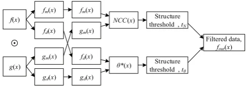
Fig. 1. The procedure of the template-based structure filtering.
2.4 Template-based filtering of vector field inCl2,0
According to the discussion above, we can design the template-based filtering algorithm (Fig. 1). The original vec-tor field data are first split into the modulus field and the unit length direction field. Since the modulus field is scalar field, we use the NCC computation algorithm proposed by Yoo and Han (2009). For the unit length direction field, the optimized angle difference field is first estimated by the SVD method. Then, we can apply a certain threshold on the NCC similar-ity NCC(x)and the angleθ∗(x)(e.g. a amplitude correlation more than 0.6 and the angular difference is less than 45◦) to extract the features according to the relations between the original and template data.
3 Experiments
3.1 Data
Global wind filled and the El Ni˜no Modoki event are studied. The 0.5◦ Grided Global Average QuikSCAT Surface Wind
Velocity Field data during May 2002 to March 2003 are used as the original data, and the Ni˜no 3.4 region of the composite El Ni˜no Modoki spatial pattern (Wang and Xin, 2013), which averages the NCEP-NCAR reanalysis wind velocity vector data during the seven El Ni˜no Modoki events, are used as the template. Since the composed wind field data (2.5◦×2.5◦) have a lower spatial resolution than the QuikSCAT wind ve-locity field data (0.5◦×0.5◦), the composite data are first lin-early interpolated in the 0.5◦×0.5◦grid.
3.2 The directional filtering with parallel template
Clifford convolution with a parallel template can extract the direction information of the vector field. A 11×11 paral-lel templateT (x) is generated with T (x)=sin[θ (x)]e1+
cos[θ (x)]e2by assigning each point of a constant 2-D vector.
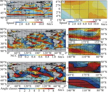
The north direction is set asθ (x)=0◦. Therefore, the tem-plate is directly northward. The directional part of the modi-fied correlation product indicates the direction of the angular difference from the north. We also compute the direction an-gle with the formula ofθ (x)=arctan(y/x)for comparison, wherexandyare the longitudinal and latitudinal projection of the normalized direction vector in each point (Fig. 2).
The overall spatial patterns of the angle value calculated from both the convolution and the original data are very sim-ilar. This proves the correctness of our method. Furthermore, the highlighted area suggest our method will produce less singularities than the direct computation. The zonal distri-bution of the global wind (e.g. Western wind zone, South-east trade wind zone etc.) can be clearly revealed, and from east to central Pacific (10◦S∼10◦N, 120◦E∼180◦), there are clearly boundaries of eastern and western wind. This area is also the birth place of El Ni˜no event and a place that has drastic changes and large influence on global climate. 3.3 The El Ni ˜no global impaction pattern extraction
A time slice (September 2002) of the original wind field, the template data, the NCC coefficient and the directional clas-sified angular coefficients are depicted in Fig. 3. The area with higher NCC coefficient may be strongly affected by this El Ni˜no event. The high impact regions are located in the Equatorial Pacific between 30◦S∼30◦N and the east coastal regions of the main continents (Fig. 3c). The value ofθ∗(x)
reveals the angular relationship between the original data and the El Ni˜no Modoki template, which indicate the directional structure change. For better expression, we classify the angu-lar differences as eight directions. The direction classification of the filtered wind field is expressed in Fig. 3d.
The directional pattern of the wind field in September 2002 and the template clearly show distinct spatial distribu-tion patterns in different areas. There are more eastward re-gions (in cold color) than westward rere-gions (in warm color) in the whole global ocean. However, significant westward re-gions exist in the Pacific and Indian oceans, which suggests the closed linkage with ENSO. The most obvious westward region is located at East Pacific, east coast of South Amer-ican, Africa, Asia, Australia and the west coast of Europe. The September 2002 is the forming stage of the El Ni˜no event and the ENSO influences in these places are much stronger. The boundaries between the eastward and westward regions in central and east Pacific also have very similar structure to that of the weak El Ni˜no composed by SST anomalies (Wang and Fiedler, 2006). Yu et al. (2012) suggests its SST anomaly center located near the coast of South America.
2 3 4 5 6m/s 0°
90°S
60°E 120°E 180° 120°W 60°W 0° 6
60°S 30°S 0 30°N 60°N 90°N
130°E 160°E 170°W5°S 15°N 35°N
170°W 140°W 110°W45°S 25°S 5°S
0 1
Angle (rad)
6m/s 0°
90°S
60°E 120°E 180° 120°W 60°W 0° 60°S
30°S 0 30°N 60°N 90°N
130°E 160°E 170°W5°S 15°N 35°N
170°W 140°W 110°W45°S 25°S 5°S
Angle (rad) (a)
(b)
2 3 4 5 6
0 1
A1
A2
B2 B1
Fig. 2. The direction pattern comparison. (a) is the angle value calculated by optional rotor estimation, and (b) is calculated with the original vector data.
6m/s 0°
90°S
120°E 120°W 0°
45°S 0 45°N 90°N
Speed 170°WSpeed 150°W
4°S 2°S 0 2°N 4°N
0 2.0 4.0 6.0 8.0 10.0 2.0 6.0 8.0 10.0
0
Niño3.4
130°W 6m/s
6m/s
6m/s
(a) (b)
140°W 110°W 80°W
30°S 10°S 10°N
145°E 175°E 155°W
10°N 30°N 50°N
0.2 0.4 0.6 0°
90°S
60°E 120°E 180° 120°W 0°
0.8 60°S
30°S 0 30°N 60°N 90°N
1.0 0.0
NCC
140°W 110°W 80°W
60°W
145°E 175°E 10°N
30°N
10°N 50°N
30°S 10°S 10°N
0° 60°E 120°E 180° 120°W
1 2 3 4 5 6 7 8
Angle classes 60°W
(d)
0° (c)
90°S 60°S 30°S 0 30°N 60°N 90°N
−3 −2 −1 0 1 2 3 −3
−2 −1 0 1 2
3 |F{ux}|2+|F{ux}|2
ky
(cell
-1)
kx(cell-1)
−3 −2 −10 1 2 3
ky
(cell
-1)
−3 −2 −1 0 1 2 3
ky
(cell
-1)
−3 −2 −1 0 1 2 3 kx(cell-1)
−3 −2 −1 0 1 2 3 kx(cell-1)
|F{ux}|2+|F{ux}|2 |F{ux}|2+|F{ux}|2
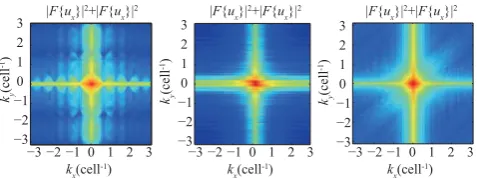
Fig. 4. The 2-D spectrum of original data (left), the template (mid-dle) and the filtered field (right). The spectrum is the squared sum of the 2-D Fourier spectrum of the vectors projected in the two di-rections.
However, the direction distribution is clear and strengthened in the spectrum of the filtered field. These characteristics sug-gest the modified correlation product can be used for pat-tern extraction which integrated both the amplitude and di-rectional part of the two vector fields.
3.4 The evolution of high El Ni ˜no impact area
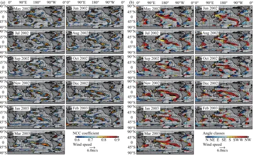
Since both the NCC and the angular filtering can provide clear signals from vector field with template-based filtering, we can explore the tempo-spatial evolution characteristics of the 2002/03 El Ni˜no event. The NCC coefficients changing with time indicate the amplitude similarity structure evolu-tion, which may mainly suggest the strength of the El Ni˜no event. And changing in the directional field classification in-dicates the directional effect evolution. In addition, the NCC threshold of NCC>0.6 is chosen to select the region highly related to or affected by the El Ni˜no event. In the region of high NCC (Fig. 5a), the angular fields are divided within eight directional classes for better visualization (Fig. 5b). The distributions of the directions as well as the NCC coefficients are also expressed with the windrose plot, in which, the fre-quencies of the number of grid in each direction are counted and the associated NCC coefficients are expressed with the colorbar (Fig. 6).
The NCC coefficients suggest the structure change from May 2002 to March 2003. This El Ni˜no event is strongly as-sociated with active phases of the MJO (Madden–Julian Os-cillation), an eastward propagating pattern affecting surface winds over the warm pool (Zhang, 2005). The characteris-tics of the MJO and its effects on surface wind can also be partially revealed in the data of NCC filtering. Several con-vective high NCC regions in the Pacific Ocean follow the eastward propagation of MJO. In May and June 2002, two of the highest NCC centers in the Pacific region appear in (10◦N, 170◦E) and (15◦S, 130◦W). But in July 2002 these two centers moved to (15◦N, 175◦E) and (25◦S, 115◦W). The whole high NCC regions in Pacific also totally show a clearly northeastward trend.
From August to October in 2002, the MJO related convec-tion is growing weak. However, the original isolated peaks
in the south ocean and the north Pacific are becoming con-nected, which suggests a global strengthening impact of the El Ni˜no. Episodic forcing associated with the MJO helped to “kickstart” the 2002/03 El Ni˜no (McPhaden, 2004), but then large-scale ocean–atmosphere feedbacks became the dominant forces that amplified and sustained the El Ni˜no. In the maximum development of this event in October– December 2002, the area of the high NCC region also grows rapidly. In October 2002, in the Pacific region there are al-ready two continuous zones that cross from 150◦E∼90◦W. The slope of the El ni˜no impact zone is even flatter. A strong similarity burst in the Pacific in November–December 2002 witnessed the amplification of the westerly wind bursts as-sociated with the El Ni˜no. And from January 2003, the area of the high NCC region declines. The termination of this El Ni˜no event starts.
3.5 The angular evolution of the El Ni ˜no event
By classifying the direction distributions in the region of high NCC with the angular filtering results (Fig. 6), the highest NCC regions locate in Pacific, and the major direction pat-tern is northwestward. Compared to the shape and structure change of the high NCC region, the northwestward direction propagation is stable over time. In the boreal summer 2002, the MJO was dominated by a strong eastward component, probably driven by the abnormally high SSTs in the central Pacific (McPhaden, 2004). And in July 2002, the directional filtering result suggests the eastward becomes strong, which can be well compared with the observation results.
The center where the El Ni˜no event developed is also a key problem for different patterns of the El Ni˜no events. Existing literatures heavily argue the differences among the east Pa-cific (EP) El Ni˜no and central PaPa-cific (CP) El Ni˜no. In our angular direction classification, the central Pacific is located at the boundaries of the eastward and westward propagation. Other indicators also suggest the El Ni˜no event was charac-terized by very high sea surface temperatures (SSTs) in the central Pacific (Kug et al., 2010). These further support that the central Pacific is the source of this El Ni˜no event evo-lution. From the directional classification evolution we can also find the main propagation direction is almost stable over time (Fig. 7), although the original direction of the wind field changes continuously throughout time. In most time slices, the majority direction is the Northwest. The only exception is the July 2002, and there are opposite El Ni˜no propagation directions on the east coast of China compared with that in North American. The influence of the heat and water trans-portation situation is also opposite (Cook et al., 2007).
4 Conclusions
0° 90°E 180° 90°W 0° 0° 90°E 180° 90°W 0°
(a) (b)
N NE E SE S SWW NW Jun 2002
Jul 2002 May 2002
Aug 2002
Sep 2002 Oct 2002
Nov 2002 Dec 2002
Jan 2003 Feb 2003
Mar 2003
Jun 2002
Jul 2002 May 2002
Aug 2002
Sep 2002 Oct 2002
Nov 2002 Dec 2002
Jan 2003 Feb 2003
Mar 2003 0°
90°S
90°E 180° 90°W 0°
45°S 0 45°N 90°N 90°S 45°S 0 45°N 90°N 90°S 45°S 0 45°N 90°N 90°S 45°S 0 45°N 90°N 90°S 45°S 0 45°N 90°N 90°S 45°S 0 45°N 90°N 90°S 45°S 0 45°N 90°N 90°S 45°S 0 45°N 90°N 90°S 45°S 0 45°N 90°N 90°S 45°S 0 45°N 90°N 90°S 45°S 0 45°N 90°N 90°S 45°S 0 45°N 90°N 0° 90°E 180° 90°W 0°
6.0m/s Angle classes
Wind speed 0.7 0.8 0.9
0.6
6.0m/s NCC coefficient
Wind speed
Fig. 5. The filtered results of modified correlation product with NCC>0.6 during May 2002 to March 2003. (a) is the NCC filtering results, and (b) is the direction classification filtering results.
N NE E SE S SW W NW N NE E SE S SW W NW N NE E SE S SW W NW N NE E SE S SW W NW N NE E SE S SW W NW N NE E SE S SW W NW
0.9 - 0.950.95 - 1.0
0.85 - 0.9 0.8 - 0.85 0.75 - 0.8 0.7 - 0.75 0.65 - 0.7 0.6 - 0.65 N NE E SE S SW W NW N NE E SE S SW W NW N NE E SE S SW W NW N NE E SE S SW W NW N NE E SE S SW W NW
May 2002 Jun 2002 Jul 2002 Aug 2002
Sep 2002 Oct 2002
NCC Nov 2002 Dec 2002
Jan 2003 Feb 2003 Mar 2003 20 10 0 20 10 0 20 10 0 20 10 0 20 10 0 20 10 0 20 10 0 20 10 0 20 10 0 20 10 0 20 10 0
Fig. 6. The direction and NCC distribution of high NCC (>0.6) fil-tering results. The direction of the windrose indicates the evaluated direction calculated by the modified correlation product, and the ve-locity of the windrose suggests the magnitude of NCC.
with the NCC and the SVD-based mean angle difference es-timation method, both the amplitude and directional relations can be analyzed synchronously. The structure filtering algo-rithm can reveal both the modulus similarities as well as the angular distribution. The method can give smooth and con-tinuous result, which may be helpful for vector data segmen-tation or classification. Future improvements, such as intro-ducing more comprehensive correlation indexes as well as more stable and accurate amplitude correlation and angular estimation model, will greatly extend the application area.
Acknowledgements. This work was supported by the NSCF Project
(Grant No. 41201377, 41231173) and NCET program (Grant No. NCET-12-0735).
Edited by: H. J. Fernando
Reviewed by: two anonymous referees
References
Brassington, G. B., Summons, N., and Lumpkin, R.: Observed and simulated Lagrangian and eddy characteristics of the East Aus-tralian Current and the Tasman Sea, Deep-Sea Res. Part II, 58, 559–573, 2011.
Bujack, R., Scheuermann, G., and Hitzer, E.: Detection of to-tal rotations on 2D-vector fields with geometric correlation, in: AIP Conference Proceedings, edited by: Sivasundaram, S., vol. 1493, 190–199, AIP, available at: http://link.aip.org/link/APC/ 1493/190/1, 2012.
Cook, E. R., Seager, R., Cane, M. A., and Stahle, D. W.: North American drought: Reconstructions, causes, and consequences, Earth-Sci. Rev., 81, 93–134, 2007.
De Bie, H., De Schepper, N., and Sommen, F.: The class of Clifford-Fourier transforms, J. Clifford-Fourier Analys. Appl., 17, 1198–1231, 2011.
Dorst, L., Fontijne, D., and Mann, S.: Geometric algebra for com-puter science: An object-oriented approach to geometry, Morgan Kaufmann, 2007.
Ebling, J. and Scheuermann, G.: Clifford Fourier transform on vec-tor fields, IEEE Trans. Vis. Comput. Graphics, 11, 469–479, 2005.
Ebling, J. and Scheuermann, G.: Template matching on vector fields using Clifford algebra, in: Proceedings 17th IKM, edited by: G¨urlebeck, K. and K¨onke, C., 1–25, 2006.
Hestenes, D. and Sobcyk, G.: Clifford algebra to geometric calcu-lus, D. Reidel, Dordrecht, Holland, 1984.
Kug, J.-S., Ahn, M.-S., Sung, M.-K., Yeh, S.-W., Min, H.-S., and Kim, Y.-H.: Statistical relationship between two types of El Ni˜no events and climate variation over the Korean Peninsula, Asia-Pac. J. Atmos. Sci., 46, 467–474, 2010.
Lewis, J.: Fast normalized cross-correlation, in: Proc. Vision Inter-face’95, 120–123, 1995.
Luo, W., Yuan, L. W., Yu, Z. Y., Yi, L., and L¨u, G. N.: Multi-dimensional vector field convergence-divergence structure adap-tive template matching method, Acta Electron. Sin., 40, 1729– 1734, 2012.
McPhaden, M. J.: Evolution of the 2002/03 El Ni˜no, Bull. Am. Me-teorol. Soc., 85, 677–695, 2004.
Mendoza, C., Mancho, A. M., and Rio, M.-H.: The turnstile mech-anism across the Kuroshio current: analysis of dynamics in al-timeter velocity fields, Nonlin. Processes Geophys., 17, 103–111, doi:10.5194/npg-17-103-2010, 2010.
Paulus, C. and Mars, J. I.: New multicomponent filters for geo-physical data processing, IEEE Trans. Geosci. Remote Sens., 44, 2260–2270, 2006.
Tafti, P. D. and Michael, U.: On regularized reconstruction of vector fields, IEEE Trans. Image Process., 20, 3163–3178, 2011. Wang, C. and Fiedler, P.: ENSO variability and the eastern tropical
Pacific: A review, Prog. Oceanogr., 69, 239–266, 2006. Wang, C. and Xin, W.: EL Ni˜no Modoki I and II classifying by
dif-ferent impacts on rainfall in Southern China and typhoon tracks, J. Climate, 26, 1322–1338, 2013.
Yoo, J. C. and Han, T. H.: Fast normalized cross-correlation, Cir-cuits Syst. Signal Process., 28, 819–843, 2009.
Yu, J.-Y., Zou, Y., Kim, S. T., and Lee, T.: The changing impact of El Ni˜no on US winter temperatures, Geophys. Res. Lett., 39, L15702, doi:10.1029/2012GL05248, 2012.
Yu, Z. Y., Yuan, L. W., L¨u, G. N., Luo, W., and Xie, Z. R.: Coupling characteristics of zonal and meridional sea level change revealed by satellite altimetry data and their response to ENSO events, Chinese J. Geophys., 54, 1972–1982, 2011.
Yuan, L., Yu, Z., Luo, W., Yi, L., and Hu, Y.: Pattern forced geo-physical vector field segmentation based on clifford FFT, Com-put. Geosci., 60, 63–69, doi:10.1016/j.cageo.2013.05.007, 2013. Zhang, C.: Madden-Julian oscillation, Rev. Geophys., 43, RG2003,