www.atmos-meas-tech.net/10/1707/2017/ doi:10.5194/amt-10-1707-2017
© Author(s) 2017. CC Attribution 3.0 License.
Assessing the accuracy of microwave radiometers and radio acoustic
sounding systems for wind energy applications
Laura Bianco1,2, Katja Friedrich3, James M. Wilczak2, Duane Hazen1,2, Daniel Wolfe1,2, Ruben Delgado4, Steven P. Oncley5, and Julie K. Lundquist3,6
1Cooperative Institute for Research in Environmental Sciences (CIRES), Boulder, CO, USA 2National Oceanic and Atmospheric Administration, Earth Systems Research Laboratory, Physical Science Division, Boulder, CO, USA
3Department of Atmospheric and Oceanic Sciences, University of Colorado, Boulder, CO, USA 4Atmospheric Physics Department, University of Maryland, Baltimore County, Baltimore, MA, USA 5National Center for Atmospheric Research, Boulder, CO, USA
6National Renewable Energy Laboratory, Golden, CO, USA
Correspondence to:Laura Bianco ([email protected])
Received: 28 September 2016 – Discussion started: 12 October 2016 Revised: 6 April 2017 – Accepted: 12 April 2017 – Published: 9 May 2017
Abstract. To assess current remote-sensing capabilities for wind energy applications, a remote-sensing system evalua-tion study, called XPIA (eXperimental Planetary boundary layer Instrument Assessment), was held in the spring of 2015 at NOAA’s Boulder Atmospheric Observatory (BAO) facil-ity. Several remote-sensing platforms were evaluated to de-termine their suitability for the verification and validation processes used to test the accuracy of numerical weather pre-diction models.
The evaluation of these platforms was performed with re-spect to well-defined reference systems: the BAO’s 300 m tower equipped at six levels (50, 100, 150, 200, 250, and 300 m) with 12 sonic anemometers and six temperature (T) and relative humidity (RH) sensors; and approximately 60 radiosonde launches.
In this study we first employ these reference measurements to validate temperature profiles retrieved by two co-located microwave radiometers (MWRs) as well as virtual temper-ature (Tv) measured by co-located wind profiling radars equipped with radio acoustic sounding systems (RASSs). Results indicate a mean absolute error (MAE) in the temper-ature retrieved by the microwave radiometers below 1.5 K in the lowest 5 km of the atmosphere and a mean absolute er-ror in the virtual temperature measured by the radio acoustic sounding systems below 0.8 K in the layer of the atmosphere covered by these measurements (up to approximately 1.6–
2 km). We also investigated the benefit of the vertical veloc-ity correction applied to the speed of sound before computing the virtual temperature by the radio acoustic sounding sys-tems. We find that using this correction frequently increases the RASS error, and that it should not be routinely applied to all data.
1 Introduction
While the increasing deployment of wind turbines increases society’s reliance on renewably generated electricity, the need for accurate forecasts of that power production is also growing (Marquis et al., 2011). Improving wind forecasts at hub height remains the top priority, but challenges de-rive from the complexity of physical processes occurring at a wide range of spatial and temporal scales. Fundamental to understanding and accurately forecasting these processes is the accurate measurement of the atmospheric parameters such as wind, temperature, and humidity in four-dimensional space. Assessing the capability and accuracy of remote-sensing instruments to capture planetary boundary layer and flow characteristics was one goal of the Department of En-ergy and NOAA-sponsored eXperimental Planetary bound-ary layer Instrumentation Assessment (XPIA; Lundquist et al., 2016) campaign conducted in the spring of 2015 at the Boulder Atmospheric Observatory (BAO), located in Erie, Colorado (∼20 km east of Boulder and ∼30 km north of Denver).
Herein, we address some of the objectives of the XPIA campaign – determining the accuracy of temperature (T), water vapor density (WVD), and relative humidity (RH) pro-files from state-of-the-art remote-sensing instruments such as microwave radiometers (MWRs) and Wind Profiling Radars (WPRs) equipped with a Radio Acoustic Sounding System (RASS), and assessing the capability of these active and pas-sive remote-sensing instruments to provide accurate informa-tion on atmospheric stability condiinforma-tions in the lower atmo-spheric boundary layer. These remote-sensing instruments operated side by side during XPIA and are compared to in situ observations from instruments mounted on a 300 m me-teorological tower and radiosondes.
Several studies have focused on evaluating the accuracy of temperature, water vapor density, and humidity retrieved by MWRs (e.g., Güldner and Spänkuch, 2001; Liljegren et al., 2001; Ware et al., 2003; Crewell and Löhnert, 2007; Ci-mini et al., 2011; Friedrich et al., 2012; Löhnert and Maier, 2012) and virtual temperature (Tv) retrieved by WPRs with RASS (May et al., 1989; Moran and Strauch, 1994; Angevine et al., 1998; Görsdorf and Lehmann, 2000). Studies evaluat-ing the accuracy of MWR measurements usevaluat-ing radiosonde observations show consistent results with differences of 1– 2 K in temperature, < 0.4 g m−3 in water vapor density, and < 20 % in humidity for most weather conditions (Güldner and Spänkuch, 2001; Liljegren et al., 2001; Ware et al., 2003; Crewell and Löhnert, 2007; Cimini et al., 2011; Löhnert and Maier, 2012). Similar results were derived from com-parisons between MWR and in situ tower observations with differences in temperature ranging from 0.7–1.7 K (Crewell and Löhnert, 2007; Friedrich et al., 2012). Studies evaluat-ing the accuracy of RASS measurements usevaluat-ing radiosonde and in situ tower observations show root mean square differ-ences of below 1◦C in virtual temperature (May et al., 1989;
Moran and Strauch, 1994; Angevine et al., 1998). Variations in the results were often a function of various factors such as height above ground, season, topography, abrupt changes in the lapse rate, and regional differences in the surrounding vegetation.
The analysis presented here builds on the results of these previous studies, but also focuses on several unique aspects. First, in our study we provide a comprehensive assessment and comparison of the accuracy of active (two different RASS systems operating side by side in similar modes) and passive (two identical MWRs operating side by side in iden-tical modes) remote-sensing instruments operated over the period of the XPIA campaign under various meteorological conditions, including cold stable air masses, downslope wind conditions, convective conditions, and rain and snow con-ditions. The accuracies of the retrievals for the two MWR systems were compared to each other as well as to several in situ radiosonde soundings and to the tower observations. Virtual temperatures from a 915 MHz WPR with RASS and a 449 MHz WPR with RASS were also analyzed and compared to in situ radiosonde soundings and tower observations. A second important contribution of this study is to specifically investigate and compare the ability of these active and pas-sive remote-sensing instruments to measure lapse rate to be used, among others, for wind energy applications. Knowing the atmospheric stability is indubitably important for wind energy applications such as wind turbine operations, as atmo-spheric turbulence and wind shear are affected by changes in atmospheric stability. Furthermore, as found in Warthon and Lunquist (2012), and Vanderwende and Lundquist (2012), at-mospheric stability impacts both turbine power production and wake characteristics (Hansen et al., 2012).
This paper is organized as follows: Sect. 2 summarizes the experimental design and instrument characteristics; Sect. 3 and 4 assesses the accuracy of temperature and lapse rates derived from MWRs and RASSs, respectively; and in Sect. 5 water vapor density and humidity from the MWRs are com-pared to in situ measurements. Finally, conclusions are pre-sented in Sect. 6.
2 Experimental design, instruments, and methods 2.1 Experimental design
Figure 1.Instruments used in this study. From the left: 300 m equipped meteorological tower (photo credit: Katie McCaffrey), radiosonde, 2 MWRs, 915 MHz and RASS system (photo credit: Katie McCaffrey), 449 MHz and RASS system (photo credit: Katie McCaffrey).
and their integration into the XPIA campaign can be found in Lundquist et al. (2016). The MWRs and WPR–RASSs operated side by side (few meters apart) at the visitor cen-ter, at about 600 m southwest of the 300 m meteorological tower. Radiosondes were launched from the visitor center in March (38 soundings), while the remaining 23 soundings were launched in April and May from the water tank site 1000 m to the southeast of the visitor center (see Fig. 1 in Lundquist et al., 2016 for details).
2.2 In situ observations: radiosonde and 300 m meteorological tower
Radiosondes were launched during fair weather conditions at 08:00 (14:00), 12:00 (18:00), 16:00 (22:00), and 20:00 (02:00) LT (UTC) between 9–19 March (38 soundings), 15 and 20–22 April (10 soundings), and 1–4 May (13 sound-ings) providing, among others, vertical profiles of tempera-ture, dewpoint temperatempera-ture, and relative humidity between the surface and > 10 km above ground level (a.g.l.). Fourteen of these soundings were released during stable atmospheric conditions, while the remaining 47 were launched during un-stable conditions.
Two types of sounding systems were used during the cam-paign: the National Center for Atmospheric Research’s Mo-bile GPS Advanced Upper-Air Sounding System (MGAUS) was used in March (with a 1 s temporal resolution and an ac-curacy of 0.25◦C on temperature and of 1.5 % on relative hu-midity) for launches from the visitor center, while the Vaisala MW31 DigiCORA sounding system was used in April and May (with a 2 s temporal resolution and an accuracy of 0.5◦C on temperature and of 5 % on relative humidity) for launches from the water tank site.
The 300 m meteorological tower was equipped with tem-perature and relative humidity sensors at six levels (50, 100, 150, 200, 250, and 300 m) operating continuously at a tem-poral resolution of 1 s. Temperature was measured with an accuracy better than 0.1 K (Horst et al., 2016).
2.3 Microwave radiometers
Two Radiometrics MWRs, one operated by NOAA (referred to as the NOAA MWR hereafter) and one operated by the University of Colorado (CU MWR), ran side by side with
identical configurations. Prior to the experiment, both MWRs were calibrated using an external liquid nitrogen target and an internal ambient target (Han and Westwater, 2000) and thoroughly serviced (sensor cleaning, radome replacement, etc.). After calibration, we compared the brightness tem-peratures of the two MWRs for each retrieved channel for 1 day, finding almost all channels in good agreement (with differences of ∼2 K for channels 51.248, 51.760, 52.280, 56.020, 57.288, 57.964, and 58.800 GHz; differences of ∼1 K for channels 22.500, 26.234, 30.000, 52.804, 53.848, and 56.660 GHz; while the remaining channels did not show appreciable differences). However, even a small difference might be enough to skew the retrieval algorithms slightly, contributing to the explanation of some of the differences be-tween the two instruments we will find later in the analysis.
the 15◦elevation scans provide higher accuracy during pre-cipitation compared to the zenith observations by minimizing the effect of liquid water and ice on the radiometer radome (Xu et al., 2014).
The nominal vertical levels of the retrieved profiles ranged from 50 m between the surface and 0.5 km a.g.l., 100 m between 0.5 and 2 km a.g.l., and 250 m between 2 and 10 km a.g.l. Note that we will refer to these nominal lev-els as vertical resolution throughout the paper. Both instru-ments were also equipped with a rain sensor and a surface sensor for observations of temperature, pressure, and rela-tive humidity. These surface observations serve as a bound-ary condition for the neural network approach. Since the sur-face sensor from the NOAA MWR was broken between 5 and 27 April, the intercomparison for the NOAA radiometer focuses solely on observations collected between 9 March–4 April and 28 April–7 May 2015, while the intercomparison for the CU radiometer includes all dates between 9 March and 7 May 2015.
2.4 WPR–RASS
Wind profiling radars are primarily used to measure the verti-cal profile of the horizontal wind vector (Strauch et al., 1984; Ecklund et al., 1988). The remote measurement of virtual temperature in the lower atmosphere is achieved with the as-sociated RASS, co-located with the WPR. Usually a WPR– RASS system is set up to operate in wind mode for a large fraction of each hour and in RASS mode for the remaining small fraction. When the system is in RASS mode, the RASS emits a longitudinal acoustic wave upward in the air that gen-erates a local compression and rarefaction of the ambient air. These density variations are tracked by the Doppler radar, and the speed of sound is measured. From the measurement of the speed of sound, the virtual temperature in the boundary layer can be obtained (North et al., 1973).
The 915 MHz WPR RASS settings were selected to sam-ple the boundary layer from 120 to 1618 m in the vertical with a 62 m resolution, while the 449 MHz WPR RASS sam-pled the boundary layer from 217 to 2001 m with 105 m res-olution.
Several factors can undermine the accuracy in Tv mea-surements from RASSs. For example, vertical velocity can influence the accuracy of RASS measurements (May et al., 1989; Moran and Strauch, 1994) because the apparent speed of sound measured by the radar is equal to the sum of the true speed of sound and the vertical air velocity. Previous studies (Moran and Strauch, 1994; Angevine and Ecklund, 1994; Görsdorf and Lehmann, 2000) have found conflict-ing results on the overall accuracy of Tv measurements by RASSs from correcting the speed of sound for the vertical ve-locity. Görsdorf and Lehmann (2000) found that the vertical velocity correction improves the accuracy of RASS temper-ature measurements only in situations when the error of the measured vertical velocities is smaller than the magnitude of
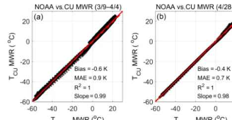
Figure 2.Comparison between temperature observed by CU MWR and NOAA MWR between(a)9 March–4 April and(b)28 April–7 May, 2015. The missing days in April coincide with the failure of the NOAA MWR surface sensor. A 1-to-1 line is indicated in solid red, and the regression is shown by the dashed red line.
the vertical velocity itself. This situation is more likely to oc-cur under unstable conditions in the boundary layer. In some cases, they found that this correction can decrease the ac-curacy of RASS, especially in situations with only light hori-zontal winds and a lower reliability of vertical wind measure-ments. Our systems provided both corrected and uncorrected vertical velocity, enabling us to investigate the accuracy of RASS measurements ofTv, both corrected and uncorrected for vertical air motion.
Since the volumes sampled by the MWRs and RASSs are substantially larger than those sampled by the soundings or the tower-based measurements, vertical averaging and linear interpolation were used to facilitate comparison. Particularly, when comparing measurements from MWRs and RASSs to sounding observations, we averaged the data of the sound-ings over the heights of the MWRs and RASSs. When com-paring measurements from RASSs to the tower observations we linearly interpolated the data of the tower over the heights of the RASSs, while when comparing measurements from the MWRs to the tower observations no spatial interpola-tion or averaging was applied since MWR-derived temper-ature levels (0, 50, 100, 150, 200, 250, 300 m) were the same height levels as the in situ tower observations.
3 Accuracy of the temperature profiles 3.1 MWRs versus sounding observations
Table 1.Statistical values for the NOAA and CU MWRs vs. radiosonde observations ofT for the three periods of radiosonde launches and for the zenith and at 15◦off-zenith angles. Bias and MAE are in (K).
March (38 radiosonde) April (13 radiosonde) May (10 radiosonde)
Bias MAE R2 slope Bias MAE R2 slope Bias MAE R2 slope
CU MWR (zenith) −0.3 1.5 0.98 0.91 0.2 1.1 0.99 0.94 0.2 1.1 0.99 0.93 vs. radiosonde
CU MWR (15◦elevation) −0.8 1.5 0.98 0.93 −0.2 0.9 0.99 0.97 −0.3 1.1 0.98 0.97 vs. radiosonde
NOAA MWR (zenith) −0.5 1.4 0.98 1.03 Missing data −0.1 1 0.99 1.04 vs. radiosonde
NOAA MWR (15◦elevation) 0 1.3 0.98 0.94 0.4 1 0.98 0.97 vs. radiosonde
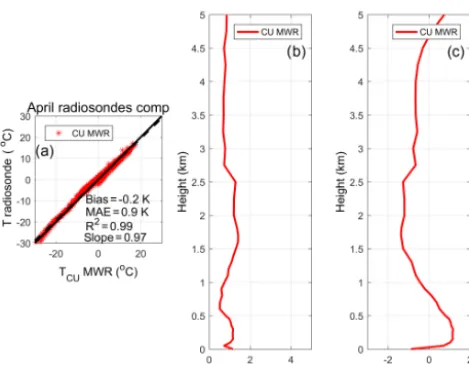
Figure 3.MWRs vs. radiosonde comparison ofT for 9–19 March including 38 radiosonde launches:(a–b)one-to-one comparisons between T observed by the radiosondes and the(a) NOAA and (b)CU MWR between the surface and 5 km a.g.l. One-on-one line is indicated as a solid black line and the regression as a dashed black line.(c–d)Vertical profiles of MAE and bias for the same variable for the NOAA MWR (blue line) and CU MWR (red line).
with exactly the same configurations (Sect. 2.3), mean ab-solute error between the two systems ranged between 0.7 and 0.9 K (Fig. 2). Note that the lack of data in April was due to a malfunctioning surface sensor of the NOAA MWR. In general, the CU MWR observed lower temperatures than did the NOAA MWR with the bias between the two instru-ments, computed as (TCU MWR−TNOAA MWR), ranging be-tween−0.4 and−0.6 K. Since the coefficient of determina-tion,R2, value was 1 during the intercomparison period, we consider the two MWRs in good agreement with each other.
For the comparison between MWRs and sounding obser-vations, the data set was divided into three periods in or-der to account for differences in the sounding systems and their locations as well as differences in the atmospheric
con-ditions. The three periods of comparison consist of March, with cooler temperatures and partially snow-covered terrain; May, with mainly warm, convective weather; and a tran-sition period in April with a mixture of cool, rainy and warm, and sunny weather. Differences in temperatures be-tween the MWRs and soundings are shown for March in Fig. 3, April in Fig. 4, and May in Fig. 5 between the surface and 5 km a.g.l. Scatter plot comparisons between soundings and the radiometer observations show that MAEs in temper-ature were slightly larger in March, ranging between 1.3 and 1.5 K (Fig. 3a–b) compared to April and May, where values ranged between 0.9 and 1.1 K (Figs. 4a, 5a–b). As previously indicated in Fig. 2, the CU MWR underestimated the temper-atures compared to the sounding observations with a bias of −0.2 to−0.8 K in March, April, and May. The NOAA MWR showed no bias (defined asTMWR−TRadiosonde)in March but overestimated temperatures in May with a bias of 0.4 K.
Temperatures derived from the MWR zenith scans were also compared to the sounding observations as presented in Table 1. In the present data set the zenith measurements per-formed better than the averaged 15◦elevation scans in terms of bias for the CU MWR in March, but not for the NOAA MWR. Despite the better coverage through the boundary layer from the 15◦elevation scans, values of MAE and R2
are surprisingly almost identical for the off-zenith and zenith MWR measurements for all three periods. Slopes are closer to 1 for the 15◦elevation scans. We decided to base the rest of the study on off-zenith-averaged observations at a 15◦ eleva-tion angle because 15◦elevation scans provide higher accu-racy compared to the zenith observations during precipitation (Xu et al., 2014).
Figure 4.Same as in Fig. 3, but for 15 and 20–22 April including 10 radiosonde launches. Note that the surface sensor of the NOAA MWR was broken between 5 and 27 April; therefore, the NOAA MWR vs. radiosonde comparison (T )over this period is not pre-sented.
MAEs were below ∼2 K at all levels not showing the in-crease in MAE that was seen in March above 3.5 km.
Bias in temperature between the MWRs and radiosondes as a function of height (Figs. 3d, 4c, 5d) showed mostly neg-ative bias in a shallow layer near the surface, positive values below ∼1 km (∼1.5 km) for the CU (NOAA) MWR, and mostly negative values above. For the March comparison, we notice that biases near the surface are opposite for the NOAA MWR and CU MWR (Fig. 3d). Since surface observations of temperature and pressure are important for the retrieval algo-rithm, we analyzed surface observations of the two MWRs. Differences in surface pressures between the two MWRs of the order of ∼6 mbar were observed for the March period and only∼1 mbar for the May period, while differences in surface temperature between the two MWRs of the order of 1.7 K were observed for the March period and only 0.8 K for the May period. We can expect that the differences of ∼6 mbar and 1.7 K between the NOAA and CU MWRs sur-face sensors might be the cause of the opposite biases found at the lowest levels of Fig. 3d, while those of Fig. 5d, af-ter the surface sensor was replaced and the differences were smaller, are of the same sign. The negative bias below 250 m is related to the surface inversions often observed at night or early morning (an example of which is shown in Fig. 6a). The details of the inversion were often in error, with the MWRs too cold at the surface and too warm above a few hundred meters due to the inversion height being displaced too high. Above 1.5 km, for some of the profiles, radiosonde temper-atures strongly differed from the MWR observations (an ex-ample of which is shown in Fig. 6b), which might be related to the presence of elevated temperature inversions that can-not be detected by the MWR or to strong observed winds
Figure 5.Same as in Fig. 3, but for the May period of 13 radiosonde launches.
Figure 6.Vertical profiles of temperature as observed by MWRs (blue line: NOAA MWR; red line: CU MWR) and radiosonde (black line) at(a)08:00 LT (14:00 UTC) on 15 March,(b)07:00 LT (13:00 UTC) on 16 March,(c)08:00 LT (14:00 UTC) on 10 March 2015, and(d)08:00 LT (14:00 UTC) on 4 May 2015.
aloft (winds larger than 10 m s−1 were observed for these circumstances, not shown) that transported the sounding far-ther away from the MWR encountering different air masses. Despite their coarser resolution, the MWRs were capable of capturing important gradients in the temperature profile – the existence or lack of surface temperature inversions at around a few hundred meters a.g.l. and the overall decrease in temperature with height (examples of which are shown in Fig. 6c–d).
Figure 7.CU MWR vs. radiosonde comparison of temperature over (a)07:00–24:00 LT,(b) 07:00–12:00 LT,(c)13:00–18:00 LT, and (d)19:00–24:00 LT between the surface and 5 km a.g.l. Data were collected on 9–19 March (38 soundings), 15 April and 20–22 April (10 soundings), and 1–4 May (13 soundings). Note that no radioson-des were launched between 01:00 and 06:00 LT. One-on-one line is indicated as a solid black line and the regression as a dashed black line.
might affect the accuracy of the temperature observation, the CU MWR retrieved temperatures were compared to the ra-diosonde temperatures at different times of the day (07:00– 12:00; 13:00–18:00; 19:00–24:00 LT), as presented in Fig. 7. This figure contains only the CU MWR because the CU and NOAA MWR were in good agreement over the two periods presented in Fig. 2 and the CU MWR has a larger data due to continuous operations. No significant differences between these different times of the day were noticed. For this reason, it can be concluded that the MWR was capable of retriev-ing temperatures with a MAE of around 1.2–1.3 K durretriev-ing different atmospheric stability conditions. In summary be-low 3.5 km we find consistent behavior of the MWRs among the different months and similar error statistics for different times of the day using MWR data up to 5 km.
3.2 RASS versus sounding observations
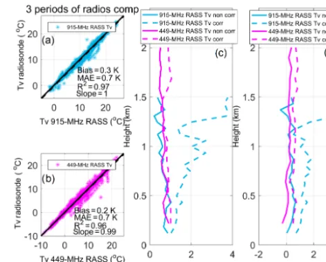
Temperature observations from the RASSs were compared to radiosonde observations in the same manner as for the MWRs. As mentioned in Sect. 2.4, we investigate the ac-curacy ofTvRASS measurements corrected and uncorrected for vertical air motion. Without the vertical velocity correc-tion (uncorrectedTv), no important differences between the three periods of radiosonde launches emerged (figure not shown). Results of the comparison between uncorrectedTv measurements from the 915 MHz and the 449 MHz RASS and all the radiosondes launched in March, April, and May
Figure 8.A 915 MHz RASS (light blue) and 449 MHz RASS (ma-genta) vs. radiosonde comparison of Tv over the three periods (March, April, and May) of radiosonde launches combined together. (a–b)One-to-one comparison between radiosonde and(a)915 MHz between 120 m and∼1.6 km a.g.l. and(b)449 MHz RASS between 217 m and∼2 km a.g.l. The correction for the vertical velocity was not applied. One-on-one line is indicated as a solid black line and the regression as a dashed black line.(c–d)Vertical profiles of MAE and bias forTvwith (dashed lines) and without (solid lines) vertical velocity correction.
are presented in Fig. 8a, b. The MAE for uncorrectedTv ob-servations was 0.7 K, with a bias of 0.2–0.3 K (defined as
TRASS−TRadiosonde).
Figure 9.CU MWR vs. tower comparison of temperature for all dates between 9 March and 7 May. (a)One-to-one comparison. One-on-one line is indicated as a solid black solid line and the re-gression as a dashed black line.(b)Vertical profiles of MAE and bias for the same variable. Temperatures were observed at the tower at 50, 100, 150, 200, 250, and 300 m a.g.l., co-located with MWR levels.
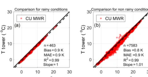
Figure 10.CU MWR vs. tower temperature measurements during (a)rainy conditions and(b)no-rain conditions as measured by the CU MWR. One-on-one line is indicated as black solid line and the regression as a dashed black line.
3.3 MWRs versus in situ tower observations
In the next step of our assessment, hourly averaged temper-atures from the in situ tower observations were compared to temperatures derived by the CU MWR for all dates between 9 March and 7 May (Fig. 9). The data set was not divided in different months since the overall statistics in Sect. 3.1 in-dicated little variation between the months. The CU MWR is in better agreement with the tower observations, with a MAE of 0.8 K (Fig. 9a), than it was with the sounding ob-servations (MAE=1.2 K; Fig. 7a). The MWR temperatures show a positive bias of 0.8 K compared to the in situ tem-perature observations. The vertical profile of MAE calcu-lated between the MWR and in situ temperature
observa-Figure 11.A 915 MHz (light blue) and 449 MHz (magenta) RASS vs. tower comparison ofTvfor all dates between 9 March and 7 May.(a–b)One-to-one comparisons between in situ tower observa-tions and uncorrectedTvobservations. One-on-one line is indicated as a solid black line and the regression as a dashed black line.(c– d)Vertical profiles of MAE and bias forTvwith (dashed lines) and without (solid lines) the vertical velocity correction. Height is a.g.l.
tions (Fig. 9b, solid line) indicates higher values of∼1 K at 150–250 m, which are exactly the heights where the MAE between the MWR and the radiosondes showed a local maxi-mum in MAE (Figs. 3c, 4b, 5c). The vertical profile of bias in temperature between MWR and in situ observations (Fig. 9b, dashed line) shows that the bias is the main contribution to the error, as the value of the bias and of the MAE are very similar to each other.
While radiosondes were only launched during rain- and snow-free conditions, the comparison with tower observa-tions (Fig. 9) contains measurements during both times with precipitation and without precipitation. A comparison be-tween MWR and in situ temperatures observations from the tower (Fig. 10) shows that the MAE was slightly lower dur-ing rainy conditions (0.8 K) than durdur-ing rain-free conditions (0.9 K), but the overall statistics are not particularly compro-mised. Note that we used the rainfall sensor that MWRs are equipped with to divide the data set between times with and without precipitation.
3.4 RASS versus in situ tower observations
Figure 12.Comparison of atmospheric lapse rate for all dates between 9 March and 7 May, 2015 for(a)CU MWR vs. tower (between first and last level of the tower measurements, 50–300 m),(b)915 MHz RASS vs. tower (between first and fourth level of the 915 MHz RASS measurements, 120–307 m), and(c)449 MHz RASS vs. tower (between first and second level of the 915 MHz RASS measurements, 217– 322 m). Negative lapse rate represents stable atmospheric conditions. One-on-one line is indicated as a solid black line and the regression as a dashed black line.
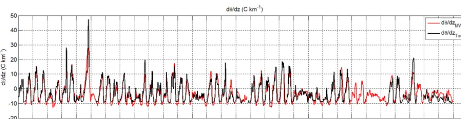
Figure 13.Lapse rate of potential temperature between 50 and 300 m a.g.l. derived from observations conducted by the CU MWR (red line) and from tower observations (black line) for all dates between 9 March and 7 May.
915 MHz RASS’s lowest four altitudes (120, 182, 245, and 307 m) and over the 449 MHz RASS’s lowest two altitudes (217 and 322 m). As for the comparison with the radiosondes presented in Sect. 3.2, the effect of applying the correction for the vertical velocity to theTvcomputation by the RASS systems was again investigated.
For the uncorrectedTv, the MAE for the RASSs were sim-ilar when using the in situ tower observations (Fig. 11a– b) as when using the radiosonde observations (Fig. 8a–b). For bias, both RASSs slightly underestimated virtual tem-peratures compared to the tower observations, with a bias of −0.1 K for the 915 MHz RASS and−0.4 K for the 449 MHz RASS. These numbers are within the expected accuracy of RASS measurements (May et al., 1989).
Vertical profiles of uncorrectedTvMAEs and biases cal-culated between the tower and both the 915 and 449 MHz RASSs (solid blue and magenta lines in Fig. 11c–d) show more accurate results than when using the RASS vertical ve-locity correction (dashed blue and magenta lines). As pre-viously found in Sect. 3.2, the vertical velocity correction
(dashed lines) was not beneficial to either the 915 MHz or the 449 MHz RASS for this data set.
We note that, comparing Figs. 3–5 to 8, and Figs. 9 to 11, the RASS has a lower error statistics than the MWRs, which was also shown in Fig. 15 of Lundquist et al. (2016).
4 Accuracy of the lapse rate
Table 2.Statistical values for the CU MWRs vs. tower observations of lapse rate (γθ= −dθ/dz)for different tower levels. Bias and MAE are in (K km−1).
Lapse rate (γθ= −dθ/dz) Lapse rate (γθ= −dθ/dz) Lapse rate (γθ= −dθ/dz) Lapse rate (γθ= −dθ/dz) between 50 and 150 m between 50 and 200 m between 50 and 250 m between 50 and 300 m
Bias MAE R2 slope Bias MAE R2 slope Bias MAE R2 slope Bias MAE R2 slope
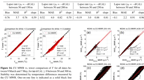
0.76 5.7 0.76 0.59 0.52 4.0 0.82 0.70 −0.19 3.0 0.88 0.81 −0.1 2.2 0.91 0.96
Figure 14.CU MWR vs. tower comparison ofT for all dates be-tween 9 March and 7 May, for(a)dϑ/dz≥0 between 50 and 300 m. Stability was determined by temperature differences measured by the CU MWR. One-on-one line is indicated as a solid black line and the regression as a dashed black line.
the ability of the MWR and the RASS to accurately capture atmospheric stability conditions in the lower boundary layer. To allow this comparison, we first computed the lapse rate of temperature (γT = −dT /dz)between 50 m and 300 m ob-served by the CU MWR and compared it with the in situ tower observations including all dates between 9 March and 7 May (Fig. 12a). Statistics indicate that for the lapse rate of temperature measured by the CU MWR and the in situ tower measurements, the MAE was about 2.1 K km−1with anR2
of 0.91.
The same analysis was performed for the lapse rate of virtual temperature (γTv= −dTv/dz)computed between the
first and fourth level of the 915 MHz RASS measurements (120–307 m) with the in situ tower observations (Fig. 12b) and the first and second level of the 449 MHz RASS mea-surements (217–322 m) with the in situ tower observations (Fig. 12c). To have a compatible comparison between the ability of the MWR at measuring lapse rate and that of the RASSs, we computed the same statistics (MAE, bias, R2, slope) presented in Fig. 12a, but first interpolating the CU MWR observations over the heights covered by the 915 MHz RASS (120–307 m) and later interpolating the CU MWR ob-servations over the heights covered by the 449 MHz RASS (217–322 m). The first gave anR2=0.89 for the CU MWR and R2=0.81 for the 915 MHz RASS, while the second gave an R2=0.79 for the CU MWR and R2=0.6 for the 449 MHz RASS, resulting in the bestR2for the MWR.
Figure 15.Comparison between(a)–(b)WVD and(c)–(d)RH ob-served by CU MWR and NOAA MWR between 9 March–4 April 2015(a, c)and 28 April–7 May 2015(b, d). The missing days in April coincide with the failure of the NOAA MWR surface sensor. One-on-one line is indicated as a solid red line and the regression as a dashed red line.
In addition to the γT and γTv, we calculated the lapse
rate of potential temperature from CU MWR measurements, as γθ= −dθ/dz (differences with the lapse rate of virtual potential temperatures were practically unnoticeable). The statistics (MAE, bias,R2, slope) were calculated forγθ us-ing different tower levels, and the results are presented in Table 2. We note that the agreement between the lapse rate of potential temperature measured by the CU MWR and the in situ tower measurements is best when it is computed be-tween 50 and 300 m (larger dz), with a coefficient of deter-mination of 0.91. A comparison between the time series of
Figure 16. MWR vs. radiosonde comparison of WVD over the March period of 38 radiosonde launches. (a)–(b) are one-to-one comparisons of WVD observed by the radiosondes and the (a)NOAA and(b)CU MWR between the surface and 5 km a.g.l. One-on-one line is indicated as a solid black line and the regression as a dashed black line.(c)Vertical profiles of MAE for the same variable.
To better quantify the differences in temperature between the CU MWR and the in situ observations, the data set was finally divided into times when the atmosphere was stable (dθ/dz≥0)and unstable (dθ/dz <0), based on the observa-tions conducted by the CU MWR presented in Fig. 13. Tem-peratures observed by the CU MWR were compared dur-ing stable and unstable conditions to in situ tower observa-tions at six height levels between 50 and 300 m. Note that stable conditions might generate profiles with an inversion at the surface. Smaller MAEs occurred in unstable condi-tions (MAE=0.8 K; Fig. 14a) compared to stable conditions (MAE=1.2 K; Fig. 14b). Larger MAE values in stable con-ditions might indicate that the MWR has difficulties accu-rately capturing the depth and the slope of the surface inver-sion. Similarly, the bias was smaller, and R2was larger, in unstable conditions compared to stable conditions.
5 Accuracy of the MWR water vapor density and humidity profiles
Differences in water vapor density and relative humidity be-tween the two MWRs were analyzed before comparing to sounding observations. Profiles derived from averaged off-zenith 15◦ elevation MWR scans between the surface and 10 km a.g.l. were compared during the time periods when both instruments were functioning (9 March–4 April 2015 in Fig. 15a–c; 28 April–7 May 2015 in Fig. 15b–d). For the WVD comparison, the MAEs for the two MWR
sys-Figure 17.Same as in Fig. 16, but for the May period of 13 ra-diosonde launches.
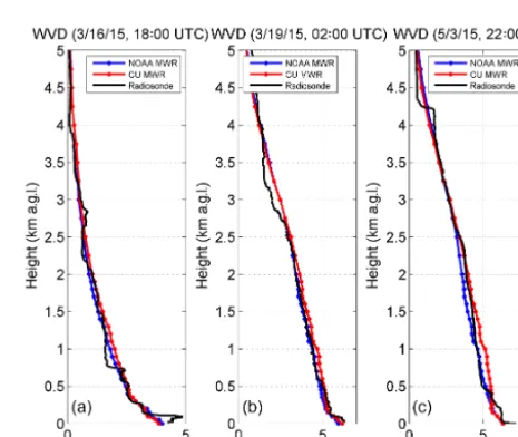
Figure 18.Vertical profiles of WVD as observed by MWRs (blue line: NOAA MWR; red line: CU MWR) and radiosonde (black line) at (a) 18:00 LT (00:00 UTC) on 16 March, (b) 02:00 LT (08:00 UTC) on 19 March, and(c)22:00 LT (04:00 UTC) on 3 May 2015.
tems were 0.1 and 0.2 g m−3, the biases were ∼0.1 g m−3, and bothR2s were close to 1 (Fig. 15a–b). For the RH com-parison, the MAEs were 4.1 and 4.8 %, the biases were 2.1 and 0.9 %, and the coefficients of determination were both 0.96 (Fig. 15c–d). The values of bias,R2, and slope indicated a good agreement between the instruments over the periods during which they were both functioning properly.
Figure 19.MWR vs. radiosonde comparison of RH over the March period of 38 radiosonde launches.(a)–(b)are one-to-one compar-isons of RH observed by the radiosondes and the(a)NOAA and (b)CU MWR between the surface and 5 km a.g.l. One-on-one line is indicated as a solid black line and the regression as a dashed black line.(c)Vertical profiles of MAE for the same variable.
and May (Figs. 16–18 for WVD; Figs. 19–21 for RH). For WVD, in March (Fig. 16) and April (not shown), MAEs for both instruments show values equal to 0.3 g m−3, also reported by Cimini et al. (2011); the biases were close to 0 g m−3, and the coefficients of determination were 0.92 (Fig. 16a–b). Vertical profiles of MAE (Fig. 16c) show val-ues of about 0.3–0.2 g m−3up to 3–3.5 km, with decreasing MAE above 3.5 km. Larger MAEs were observed for WVD in May (Fig. 17) compared to March and April. MAE is equal to 0.5 g m−3 (Fig. 17a–b), with R2 values of about 0.92. Vertical profiles of MAE in May indicate larger val-ues below 2.5 km, where WVD profiles from the sounding showed more variability, decreasing above. Overall MWRs are able to follow the radiosonde vertical profile of WVD as presented in Fig. 18, although some information is missed due to the coarser MWRs resolution compared to the resolu-tion of the sounding observaresolu-tions.
For RH, MAEs for both instruments show values below 10 % in March (Fig. 19a–b). A relatively large scatter (R2
of ∼0.8) is an indication of large variation in relative hu-midity. Some of the variability and associated large scatter might be attributed to the sounding encountering different air masses or even clouds at higher altitudes, as indicated by the vertical profiles of MAE. These profiles show that the MAEs are about 5–8 % below ∼1 km, with the MAEs continuously increasing with increasing height (Fig. 20c). Larger MAEs were observed in April (not shown) and May (Fig. 20) compared to March (Fig. 19). MAEs range between 11 % (in May) and 14 % (in April, not shown), withR2
val-Figure 20.Same as in Fig. 19, but for the May period of 13 ra-diosonde launches.
Figure 21.Vertical profiles of RH as observed by MWRs (blue line: NOAA MWR; red line: CU MWR) and radiosonde (black line) at (a)18:00 LT (00:00 UTC) on 16 March,(b)02:00 LT (08:00 UTC) on 19 March, and(c)22:00 LT (04:00 UTC) on 3 May 2015.
ues of about 0.5. Vertical profiles of MAE in April and May indicate a similar pattern compared to March. Lower val-ues (5–12 %) were observed below∼1 km, while larger val-ues occurred around 1 km and between 3 and 4 km. Since the three-dimensional humidity field is highly variable and strongly depends whether or not the instruments (both MWR and sounding) encountered clouds, the large MAEs between 1 and 4 km are most likely due to changes in air mass or the existence of clouds.
MWR humidity profiles, as seen in Fig. 21. These exam-ples show that while the MWRs are capable of reproducing the general trend compared to sounding observations, differ-ences between the MWR and the sounding can be as high as 20–25 %.
6 Conclusions
Data collected during the XPIA campaign in spring 2015 were used to assess the accuracy of temperature, water va-por density, and relative humidity profiles from two MWRs, one 915 MHz WPR–RASS system, and one 449 MHz WPR– RASS system with respect to in situ reference measurements from 61 radiosonde launches and temperature and relative humidity measurements at six different levels from a 300 m co-located atmospheric tower. Results indicate a mean abso-lute error in the temperature retrieved by the MWRs below 1.5 K for the layer of the atmosphere up to 5 km. However, the details of the inversions were consistently in error, with the MWRs too cold at the surface and too warm above 250 m. Our results revealed that the overall statistics for MWRs tem-perature measurements were slightly better for unstable con-ditions than stable concon-ditions with temperature inversions at the surface, while the overall statistics for MWR tem-perature measurements were not particularly compromised during rainy conditions compared to rain-free conditions. In addition, we find consistent behavior of the MWRs among the different months and similar error statistics for different times of the day.
For the RASSs we found a mean absolute error in the vir-tual temperature below 0.8 K in the layer of the atmosphere covered by these measurements (up to approximately 1.6– 2 km) and that using the values ofTv corrected for the ver-tical velocity can decrease temperature accuracy and should only be used with caution. For this data set, the correction for the vertical velocity applied to calculateTv was not benefi-cial to the accuracy of RASS measurements ofTvunder any weather condition. In general the RASSs have overall lower error statistics than the MWRs for the layer of the atmosphere covered by the RASSs.
We additionally assessed the accuracy of these remote-sensing instruments at measuring atmospheric stability con-ditions in the lower boundary layer, finding a coefficient of determination between the lapse rate measured by the MWR and the tower measurements over the tower levels between 50 and 300 m ranged from 0.76 to 0.91, with the best value (0.91) found when the lapse rate was computed between 50 m and 300 m (larger dz). These positive results demonstrate that profiling microwave radiometers can be useful for un-derstanding conditions that can lead to strong vertical wind shear or turbulence, which can affect the loads on rotors.
We also assessed the accuracy of MWRs at retrieving wa-ter vapor density profiles, finding a mean absolute error be-low 0.5 g m−3for the layer of the atmosphere up to 5 km.
Finally, our study unsurprisingly revealed that relative hu-midity profiles measured by the MWR lack high resolution details compared to radiosonde measurements, with differ-ences between the MWR and the sounding that can be as high as 20–25 % and on average, for the layer of the atmo-sphere up to 5 km, of the order of 8–14 %. For this reason, our future research will utilize the unique data set collected for XPIA to combine the information obtained from WPR potential refractivity profiles and from MWR potential tem-perature profiles to improve the accuracy of atmospheric hu-midity profiles (Bianco et al., 2005).
Data availability. The XPIA dataset is available to the public on-line (https://a2e.energy.gov/projects/xpia; Lundquist et al., 2016).
Competing interests. The authors declare that they have no conflict of interest.
Acknowledgements. The authors wish to acknowledge the two
anonymous Referees for the useful suggestions that improved the paper and Alex St. Pé from the University of Maryland, Baltimore County, as well as the University of Colorado Boul-der students Joseph C.-Y. Lee, Paul Quelet, Clara St. Martin, Brian Vanderwende, and Rochelle Worsnop who launched the radiosondes and Timothy Lim of NCAR for providing them careful training. We are very grateful for the assistance received from Radiometrics Corporation in setting up and comparing the two MWRs calibrations. Thanks go to the University of Colorado Boulder students Joshua Aikins and Evan Kalina who set up the CU radiometer. We express appreciation to the National Science Foundation for supporting the CABL deployments (https://www.eol.ucar.edu/field_projects/cabl) of the MGAUS radiosondes and the tower instrumentation. We thank the Left-hand Water District for providing access to the Water Tank site. We would like to acknowledge operational, technical, and scien-tific support provided by NCAR’s Earth Observing Laboratory, sponsored by the National Science Foundation, as well as by Timothy Coleman and the group of engineers of NOAA/PSD. Partial support for the UMBC deployments was provided by the Maryland Energy Administration. NREL is a national laboratory of the US Department of Energy, Office of Energy Efficiency and Renewable Energy, operated by the Alliance for Sustainable Energy, LLC. Funding for this work was provided by the US Department of Energy, Office of Energy Efficiency and Renewable Energy, Wind and Water Power Technologies Office, and by NOAA’s Earth System Research Laboratory.
Edited by: W. Shaw
References
Angevine, W. M. and W. Ecklund: Errors in radio acoustic sounding of temperature, J. Atmos. Ocean. Technol., 11, 837–842, 1994. Angevine, W. M., Bakwin, P. S., and Davis, K. J.: Wind profiler
and RASS measurements compared with measurements from a 450 m-tall tower, J. Atmos. Ocean. Technol., 15, 818–825, 1998. Bianco, L., Cimini, D., Marzano, F. S., and Ware, R.: Combin-ing microwave radiometer and wind profiler radar measurements for high-resolution atmospheric humidity profiling, J. Atmos. Ocean. Technol., 22, 949–965, 2005.
Cimini, D., Campos, E., Ware, R., Albers, S., Giuliani, G., Ore-amuno, J., Joe, P., Koch, S. E., Cober, S., and Westwater, E.: Thermodynamic atmospheric profiling during the 2010 Win-ter Olympics using ground-based microwave radiometry, IEEE T. Geosci. Remote, 99, 1–11, doi:10.1109/TGRS.2011.2154337, 2011.
Crewell, S. and Löhnert, U.: Accuracy of boundary layer tem-perature profiles retrieved with multifrequency multiangle mi-crowave radiometry, IEEE T. Geosci. Remote, 45, 2195–2201, doi:10.1109/TGRS.2006.888434, 2007.
Ecklund, W. L., Carter, D. A., and Balsley, B. B. A.: UHF wind pro-filer for the boundary layer: brief description and initial results, J. Atmos. Ocean. Technol., 5, 432–41, 1988.
Ecklund, W. L., Carter, D. A., Balsley, B. B., Currier, P. E., Green, J. L., Weber, B. L., Gage, K. S.: Field tests of a lower tropospheric wind profiler, Radio Sci., 25, 899–906, doi:10.1029/RS025i005p00899, 1990.
Friedrich, K., Lundquist, J. K., Aitken, M., Kalina, E. A., and Mar-shall, R. F.: Stability and turbulence in the atmospheric boundary layer: A comparison of remote sensing and tower observations, Geophys. Res. Lett., 39, L03801, doi:10.1029/2011GL050413, 2012.
Görsdorf, U. and Lehmann, V.: Enhanced Accuracy of RASS-Measured Temperatures Due to an Improved Range Correction, J. Atmos. Ocean. Technol., 17, 406–416, 2000.
Güldner, J. and Spänkuch, D.: Remote sensing of the thermody-namic state of the atmospheric boundary layer by ground-based microwave radiometry, J. Atmos. Ocean. Technol., 18, 925–933, 2001.
Hansen, K. S., Barthelmie, R. J., Jensen, L. E., and Sommer, A.: The impact of turbulence intensity and atmospheric stability on power deficits due to wind turbine wakes at Horns Rev wind farm, Wind Energy, 15, 183–196, doi:10.1002/we.512, 2012.
Han, Y. and Westwater, E. R.: Analysis and improvement of tipping calibration for ground-based microwave radiometers, IEEE T. Geosci. Remote, 38, 1260–1276, doi:10.1109/36.843018, 2000. Horst, T. W., Semmer, S. R., and Bogoev, I.: Evaluation of
Mechanically-Aspirated Temperature/Relative Humidity Radia-tion Shields, 18th Symposium on Meteorological ObservaRadia-tion and Instrumentation, AMS Annual Meeting, New Orleans, LA, 10–15 January 2015, available at: https://ams.confex.com/ams/ 96Annual/webprogram/Paper286839.html (last access: 4 May 2017), 2016.
Liljegren, J., Lesht, B. M., Kato, S., and Clothiaux, E.: Initial evaluation of profiles of temperature, water vapor and cloud liquid water from a new microwave profiling radiometer, in: Preprints, 11th Symp. on Meteorological Observations and In-strumentation, Albuquerque, NM, January 2001, Amer. Meteor.
Soc., 8, available at: http://radiometrics.com/data/uploads/2012/ 11/MWRP_ARM01.pdf (last access: 4 May 2017), 2001. Löhnert, U. and Maier, O.: Operational profiling of
tempera-ture using ground-based microwave radiometry at Payerne: prospects and challenges, Atmos. Meas. Tech., 5, 1121–1134, doi:10.5194/amt-5-1121-2012, 2012.
Lundquist, J. K., Wilczak, J. M., Ashton, R., Bianco, L., Brewer, W. A., Choukulkar, A., Clifton, A., Debnath, M., Delgado, R., Friedrich, K., Gunter, S., Hamidi, A., Iungo, G. V., Kaushik, A., Kosovi´c, B., Langan, P., Lass, A., Lavin, E., Lee, J. C.-Y., McCaffrey, K. L., Newsom, R. K., Noone, D. C., Oncley, S. P., Quelet, P. T., Sandberg, S. P., Schroeder, J. L., Shaw, W. J., Sparling, L., St. Martin, C., St. Pe, A., Strobach, E., Tay, K., Vanderwende, B. J., Weickmann, A., Wolfe, D., and Worsnop, R.: Assessing state-of-the-art capabilities for probing the atmo-spheric boundary layer: the XPIA field campaign, B. Am. Meteo-rol. Soc., 98, 289–314, doi:10.1175/BAMS-D-15-00151.1, 2016. Marquis, M., Wilczak, J., Ahlstrom, M., Sharp, J., Stern, A., Smith, J. C., and Calvert, S.: Forecasting the wind to reach significant penetration levels of wind energy, B. Am. Meteorol. Soc., 92, 1159–1171, doi:10.1175/2011BAMS3033.1, 2011.
May P. T., Moran, K. P., and Strauch, R. G.: The Accuracy of RASS Temperature Measurements, J. Appl. Meteorol., 28, 1329–1335, 1989.
Moran, K. P. and Strauch, R. G.: The Accuracy of RASS Tempera-ture Measurements Corrected for Vertical Air Motion, J. Atmos. Ocean. Technol., 11, 406–4016, 1994.
North, E. M., Peterson, A. M., and Parry, H. D.: RASS, a remote sensing system for measuring low-level temperature profiles, B. Am. Meteorol. Soc., 54, 912–919, 1973.
Reehorst, A. L.: Comparison of profiling microwave radiometer, aircraft, and radiosonde measurements from the Alliance Ic-ing Research Study (AIRS), NASA/TM-2001-211101, 12 pp., available at: http://ntrs.nasa.gov/archive/nasa/casi.ntrs.nasa.gov/ 20010098322.pdf, 2001.
Rosenkranz, P. W.: Water vapor microwave continuum absorption: A comparison of measurements and models, Radio Sci., 33, 919– 928, 1998.
Solheim, F., Godwin, J., and Ware, R.: Passive ground-based re-mote sensing of atmospheric temperature, water vapor, and cloud liquid water profiles by a frequency synthesized microwave ra-diometer, Meteorol. Z., 7, 370–376, 1998a.
Solheim, F., Godwin, J., Westwater, E., Han, Y., Keihm, S., Marsh, K., and Ware, R.: Radiometric profiling of temperature, water vapor and cloud liquid water using various inversion methods, Radio Sci., 33, 393–404, 1998b.
Strauch, R. G., Merritt, D. A., Moran, K. P., Earnshaw, K. B., and Van De Kamp, D.: The Colorado wind-profiling network, J. At-mos. Ocean. Technol., 1, 37–49, 1984.
Vanderwende, B. J. and Lundquist, J. K.: The modification of wind turbine performance by statistically distinct atmospheric regimes, Environ. Res. Lett., 7, 034035, doi:10.1088/1748-9326/7/3/034035, 2012.
Wharton, S. and Lundquist, J. K.: Atmospheric stability affects wind turbine power collection, Environ. Res. Lett., 7, 014005, doi:10.1088/1748-9326/7/1/014005, 2012.