https://doi.org/10.5194/npg-25-605-2018 © Author(s) 2018. This work is distributed under the Creative Commons Attribution 4.0 License.
Comparison of stochastic parameterizations in the framework
of a coupled ocean–atmosphere model
Jonathan Demaeyer and Stéphane Vannitsem
Royal Meteorological Institute of Belgium, Avenue Circulaire, 3, 1180 Brussels, Belgium Correspondence:Stéphane Vannitsem ([email protected])
Received: 2 January 2018 – Discussion started: 17 January 2018
Revised: 18 June 2018 – Accepted: 2 July 2018 – Published: 30 August 2018
Abstract. A new framework is proposed for the evaluation of stochastic subgrid-scale parameterizations in the context of the Modular Arbitrary-Order Ocean-Atmosphere Model (MAOOAM), a coupled ocean–atmosphere model of inter-mediate complexity. Two physically based parameterizations are investigated – the first one based on the singular per-turbation of Markov operators, also known as homogeniza-tion. The second one is a recently proposed parameterization based on Ruelle’s response theory. The two parameteriza-tions are implemented in a rigorous way, assuming however that the unresolved-scale relevant statistics are Gaussian. They are extensively tested for a low-order version known to exhibit low-frequency variability (LFV), and some prelimi-nary results are obtained for an intermediate-order version. Several different configurations of the resolved–unresolved-scale separations are then considered. Both parameteriza-tions show remarkable performances in correcting the impact of model errors, being even able to change the modality of the probability distributions. Their respective limitations are also discussed.
1 Introduction
Climate models are not perfect, as they cannot encompass the whole world in their description. Model inaccuracies, also called model errors, are therefore always present (Trevisan and Palatella, 2011). One specific type of model error is asso-ciated with spatial (or spectral) resolution of the model equa-tions. A stochastic parameterization is a method that allows us to represent the effect of unresolved processes into mod-els. It is a modification, or a closure, of the time-evolution equations for the resolved variables that take into account this
effect. A typical way to include the impact of these scales is to run a high-resolution model and to perform a statisti-cal analysis to obtain the information needed to compute a closure of the equations such that the truncated model is sta-tistically close to the high-resolution model. These methods are crucial for climate modeling, since the models need to remain as low resolution as possible, in order to be able to generate runs for very long times. In this case, the stochas-tic parameterization should allow for improving the variabil-ity and other statistical properties of the climate models at a lower computational cost.
The usual way to test the effectiveness of a parameter-ization method is to consider a well-known climate low-resolution model on which other methods have already been tested. For instance, several methods cited above have been tested on the Lorenz 96 model (Lorenz, 1996), see e.g., Crommelin and Vanden-Eijnden (2008); Arnold et al. (2013); Abramov (2015) and Vissio and Lucarini (2018). These approaches have also been tested in more realis-tic models of intermediate complexity that possess a wide range of scales and possibly a lack of timescale separa-tion1, for instance the evaluation of the MTV parameteri-zation on barotropic and baroclinic models (Franzke et al., 2005; Franzke and Majda, 2006). Due to the blooming of pa-rameterization methods developed with different statistical or dynamical hypotheses (i.e., weak coupling hypothesis, scale separation), new comparisons are called for.
In this work, we investigate two parameterizations in the context of the MAOOAM (Modular Arbitrary-Order Ocean-Atmosphere Model) ocean–atmosphere cou-pled model (De Cruz et al., 2016), used as a paradigm for multiscale systems. It is a two-layer baroclinic atmo-spheric model coupled to a shallow-water ocean. It has been shown to exhibit multiple timescales including a low-frequency variability (LFV) which is realistic for the midlat-itude ocean–atmosphere system (Vannitsem et al., 2015). It possesses also a wide range of behaviors depending on the chosen operating resolution (De Cruz et al., 2016). As such, it forms a nice framework for testing parameterization meth-ods on ocean–atmosphere-related problems.
The particular problem of the atmospheric impact on the ocean could be addressed in this context as in Arnold et al. (2003) and Vannitsem (2014). It is an elegant problem, with a nice timescale separation, and which dates back to the work of Hasselmann (1976). However, in the present framework, other arbitrary decompositions of the model are possible, to address other questions. For instance, one may ask the ques-tion of the influence of the fast atmospheric processes on the slower atmospheric modes as well as on the very slow ocean. This problem was already addressed by the authors in Demaeyer and Vannitsem (2017) for a particular decom-position of the atmospheric modes based on the existence of an underlying invariant manifold. The parameterization considered was the one proposed by Wouters and Lucarini (2012), and for this specific invariant manifold configuration, the stochastic parameterization is greatly simplified. Here, we extend this study by considering also the MTV parameter-ization (Franzke et al., 2005) with different arbitrary config-urations. This in particular allows us to study different cases with or without multiplicative noise.
This paper is organized as follows: in Sect. 2, we introduce briefly the MAOOAM model and its time-evolution equa-1Timescale separation, or the existence of a spectral gap, is a
crucial ingredient on which numerous parameterization methods rely.
500 hPa
0≤ y/L
≤ π ψo
0≤ x/L ≤ 2π/n
ψa3 ψa1
Perio dic
boun dary
con ditio
ns
750 hPa 250 hPa
No-flux boundary conditions
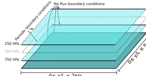
Figure 1.MAOOAM model schematic representation.
tions. In Sect. 3, we review the parameterization methods we have applied to MAOOAM and detail the model decomposi-tions into resolved and unresolved components. The results obtained with these parameterizations, with different config-urations, are presented in Sect. 4. Finally, the conclusions are provided in Sect. 5 and new work avenues are proposed.
2 The MAOOAM model
The Modular Arbitrary-Order Ocean-Atmosphere Model is a coupled ocean–atmosphere model for midlatitudes. It is com-posed of a two-layer atmosphere over a shallow-water ocean layer on aβplane (De Cruz et al., 2016). The ocean is con-sidered as a closed basin with no-flux boundary conditions, while the atmosphere is defined in a channel, periodic in the zonal direction and with free-slip boundary conditions along the meridional boundaries. The model incorporates both a frictional coupling (momentum transfer) and an energy bal-ance scheme which accounts for radiative and heat flux trans-fers between the ocean and the atmosphere. This model is de-veloped as a basic representation of the processes at play be-tween the ocean and the atmosphere, and to emphasize their impact on the midlatitude climate and weather. In particular, it has been shown to display a prominent low-frequency vari-ability in a 36-dimension model version (Vannitsem et al., 2015).
The dynamical fields of the model include the atmospheric barotropic streamfunctionψaand temperature anomalyTa= 2f0
Rθa(withf0the Coriolis parameter at midlatitude andR the Earth radius) at 500 hPa, as well as the oceanic stream-functionψo and temperature anomalyTo. In order to com-pute the time evolution of these fields, they are expanded in Fourier series with a set of functions satisfying the aforemen-tioned boundary conditions:
FPA(x0, y0)= √
2 cos(P y0), (1)
for the atmosphere and φHo,Po(x
0, y0)=2 sin(Hon
2 x
0)sin(P
oy0) (4)
for the ocean, with integer values ofM,H,P,Ho, andPoand wherex0=x/Landy0=y/Lare the non-dimensional coor-dinates on theβplane. These functions are then reordered as specified in De Cruz et al. (2016) and the fields are expanded as follows:
ψa(x0, y0, t )= na
X
i=1
ψa,i(t )Fi(x0, y0), (5)
Ta(x0, y0, t )=2f0 R
na
X
i=1
θa,i(t ) Fi(x0, y0),
ψo(x0, y0, t )= no
X
j=1
ψo,j(t ) (φj(x0, y0)−φj), (6)
To(x0, y0, t )= no
X
j=1
θo,j(t ) φj(x0, y0), (7)
with
φj= n 2π2 π Z 0 2π n Z 0
φj(x0, y0)dx0dy0, (8)
a term that allows for mass conservation in the ocean, but does not play any role in the dynamics.
By recasting these expansions into the par-tial differential equations of the model, one ob-tains a set of ODEs for its coefficients Z= ({ψa,i},{θa,i},{ψo,j},{θo,j})i∈{1,...,na}, j∈{1,...,no}:
˙
Zi=Hi+ N
X
j=1
LijZj+ N
X
j,k=1
Bij kZjZk, (9)
where N=2na+2no is the total number of coefficients. This model includes thus forcings, linear interactions and dissipations, as well as quadratic interactions representing the advection terms. Note that the full model equations of MAOOAM include quartic terms for the temperature fields, but those terms have been linearized around equilibrium tem-peratures (Vannitsem et al., 2015).
3 Model decompositions and parameterizations Now let us consider a more general system of ordinary dif-ferential equations:
˙
Z=T (Z), (10)
where Z∈RN represents the set of variables of a given model. A parameterization of the model supposes first to de-fine a decomposition of this set of variables into two differ-ent subsetsZ=(X,Y), withX∈RNXandY∈RNY. In gen-eral, this decomposition is made such that the subsetsXand
Y have strongly differing response times:τY τX (Arnold et al., 2003). However, we will assume here that this con-straint is not necessarily met, allowing for a more arbitrary split of the system variables. System (10) can then be ex-pressed as
˙
X = F (X,Y) ˙
Y = H (X,Y). (11)
The timescale of theX subsystem is typically (but not al-ways) much longer than the one of theY subsystem, and it is sometimes materialized by a parameterδ=τY/τX1 in front of the time derivativeY˙. TheXand theYvariables rep-resent respectively the resolved and the unresolved compo-nents of the system. A parameterization is a reduction of the system (11) into a closed evolution equation forXalone such that this reduced system approximates the resolved compo-nent (Arnold et al., 2003). The term “accurately” here can have several meanings, depending on the kind of problem to solve. For instance we can ask that the closed system forX has statistics that are very close to the ones of the resolved component of system (11). We can also ask that the trajecto-ries of the closed system remain as close as possible to the trajectories of the full system for long times, but this latter question will not be addressed in the present work.
More precisely a parameterization of the subsystemY is thus a relation4between the two subsystems:
Y=4(X, t ), (12) which allows us to effectively close the equations for the sub-systemX while retaining the effect of the coupling to the Y subsystem. Since the work of Hasselmann (1976), vari-ous stochastic parameterizations have been introduced (De-maeyer and Vannitsem, 2018, and Frederiksen et al., 2017, for reviews). They allow for a better representation of the variability of the processes and consider the relation (12) in a statistical sense. In this case, the aforementioned closed sys-tem forXbecomes a stochastic differential equation (SDE). If the system (11) is rewritten as
˙
X = FX(X)+9X(X,Y) ˙
Y = FY(Y)+9Y(X,Y)
, (13)
these SDEs are usually written as ˙
X=FX(X)+G(X, t )+σ(X)·ξ(t ), (14) where the matrixσ, the deterministic functionGand the vec-tor of random processesξ(t )have to be determined. We now detail in the rest of this section the two parameterizations that we will consider, namely the Wouters–Lucarini (WL) and the MTV approach.
3.1 Stochastic parameterizations
unre-solved components are weakly coupled. This method pro-posed by Wouters and Lucarini (2012) is connected to the Mori–Zwanzig formalism (Wouters and Lucarini, 2013). It has already been applied to stochastic triads (Wouters et al., 2016; Demaeyer and Vannitsem, 2018), to the Lorenz 96 model (Vissio and Lucarini, 2018) and to the MAOOAM model in the 36-variable configuration displaying LFV (De-maeyer and Vannitsem, 2017). It considers the following de-composition:
˙
X=FX(X)+ε 9X(X,Y), (15)
˙
Y =FY(Y)+ε 9Y(X,Y), (16)
whereεis a small parameter accounting for the weak cou-pling and the functionsFXandFY account for all the terms involving onlyXandY respectively.
As said above, the parameterization is based on Ruelle’s response theory, which quantifies the contribution of the per-turbations9Xand9Y to the invariant measureρof the fully coupled system (13) as
ρ=ρ0+ε δ9ρ(1)+ε2δ9,9ρ(2)+O(ε3), (17) whereρ0is the invariant measure of the uncoupled system. The two measures ρ and ρ0 are supposed to be existing, well-defined Sinai–Ruelle–Bower (SRB) measures (Young, 2002). As a result of Eq. (17), the parameterization is based on three different terms having a response similar, up to order two, to the couplings9Xand9Y:
˙
X=FX(X)+ε M1(X)+ε2M2(X, t )+ε2M3(X, t ), (18) where
M1(X)=
D
9X(X,Y)
E
ρ0,Y
(19) is an averaging term.ρ0,Y is the measure of the uncoupled systemY˙ =FY(Y). The termM2(X, t )is a correlation term:
D
M2 X(t ), t⊗M2 X(t+s), t+s
E
=
D
9X0 (X,Y)⊗9X0 φXs(X), φYs(Y)E
ρ0,Y
, (20)
where ⊗ is the outer product; 9X0(X,Y)=9X(X,Y)− M1(X)is the centered perturbation; andφsX,φYs are the flows of the uncoupled systemX˙ =FX(X)andY˙ =FY(Y). The M3term is a memory term:
M3(X, t )=
∞ Z
0
ds h(X(t−s), s), (21)
involving the memory kernel
h(X, s)=D9Y(X,Y)·∂Y9X φsX(X), φ s Y(Y)
E
ρ0,Y
. (22)
All the averages are thus taken withρ0,Y, and the termsM1, M2 andM3are derived (Wouters and Lucarini, 2012) such that their responses up to order two match the response of the perturbations9Xand9Y. Consequently, this ensures that for a weak coupling, the response of the parameterization (18) on the observables will be approximately the same as the re-sponse of the full coupled system.
3.1.2 The Majda–Timofeyev–Vanden-Eijnden (MTV) parameterization
This approach is based on the singular perturbation methods that were developed for the analysis of the linear Boltzmann equation in an asymptotic limit (Grad, 1969; Ellis and Pin-sky, 1975; Papanicolaou, 1976; Majda et al., 2001) and it has been applied to deterministic systems as well (Melbourne and Stuart, 2011; Kelly and Melbourne, 2017). These meth-ods are applicable for parameterization purposes if the prob-lem can be cast into a linear backward Kolmogorov equa-tion (Pavliotis and Stuart, 2008). Addiequa-tionally, the procedure, described in Majda et al. (2001), requires some assumptions on the timescales of the different terms of the system (13). In terms of the timescale separation parameterδ=τY/τX, the fast variability of the unresolved componentY is considered of orderO(δ−2), and the coupling terms are acting on an in-termediary timescale of orderO(δ−1):
˙
X=FX(X)+ 1
δ9X(X,Y), (23) ˙
Y= 1
δ2FY(Y)+ 1
δ9Y(X,Y) . (24) The intrinsic dynamicsFXis thus the climateO(1)timescale which one is trying to improve with the parameterization2. The term FY is defined based on which terms are consid-ered as part of the fast variability. It is then assumed that this fast variability can be modeled as an Ornstein–Uhlenbeck process. The Markovian nature of the process defined by Eqs. (23)–(24) and its singular behavior in the limit of an infi-nite timescale separation (δ→0) then allows the application of the method. More specifically, the parameterδ serves to distinguish terms with different timescales and is then used as a small perturbation parameter. In this setting, the back-ward Kolmogorov equation reads (Majda et al., 2001)
−∂ρ δ
∂s =
1
δ2L1+ 1
δL2+L3
ρδ, (25)
where the probability densityρδ(s,X,Y|t ) is defined with the final value problem f (X): ρδ(t,X,Y|t )=f (X). The density ρδ can be expanded in terms of δ and inserted in Eq. (25). The zeroth order of this equationρ0can be shown
2Note that in homogenization theoryF
to be independent of Y and its evolution given by a closed, averaged backward Kolmogorov equation (Kurtz, 1973): −∂ρ
0 ∂s = ¯Lρ
0. (26)
The precise definition of the operators Li andL¯ acting on the densities is given in Appendix A. This latter equation is obtained in the limitδ→0 and gives the sought limiting, av-eraged processX(t ). The parameterization obtained by this procedure is detailed in Franzke et al. (2005) and takes the form (14). As stated above, the parameterization itself de-pends on which terms of the unresolved component are con-sidered as fast, and some assumptions should here be made. It is the subject of the next section.
3.2 Model decompositions
As MAOOAM is a model whose nonlinearities consist solely of quadratic terms, the decomposition of Eq. (9) into a re-solved and an unrere-solved component can be done based on the constant, linear and quadratic terms of its tendencies, as in Majda et al. (2001) and Franzke et al. (2005):
˙
X=HX+LXX·X+LXY ·Y
+BXXX:X⊗X+BXXY :X⊗Y+BXY Y :Y⊗Y, (27) ˙
Y =HY+LY Y·Y+LY X·X
+BY XX:X⊗X+BY XY:X⊗Y+BY Y Y:Y⊗Y. (28) The vectors H are the constant terms of the tendencies. The matricesLgive the linear dependencies through matrix-vector products:
LXX·X i
= NX
X
j=1
LXXi j Xj . (29)
The symbol⊗is the outer product and is used to define ma-trices and tensors, e.g.,
(X⊗X)ij=XiXj and
(X⊗X⊗X)ij k=XiXjXk, (30) and “:” means an element-wise product with summation over the last and first two indices of its first and second arguments respectively3. For a rank-3 tensor and a matrix, it gives, for example,
BXXX:X⊗X i
= NX
X
j,k=1
Bi j kXXXXjXk . (31)
As we have seen in Sect. 3.1, the two parameterization meth-ods rely on a weak coupling between the components for the 3For two matricesAandB, it is thus the Frobenius inner
prod-uct:A:B=Tr
AT·B.
WL method and on a clear three-stages timescale separation for the MTV method. In some particular cases, it is possi-ble to establish an equivalence between these two assump-tions (Wouters et al., 2016). However, in general, the relation between the two is far from trivial. Timescale separation is easy to assess, by considering the decorrelation times in the output data of the model. On the other hand, weak coupling is difficult to measure in data and appears in general as a small coupling parameter resulting from the proper modeling of the components of a system.
3.2.1 Decomposition of the resolved component tendencies
This decomposition can be chosen arbitrarily since the only requirement is thatFXdepends solely onX. However, in the following (and in the provided code), we will consider that the resolved–unresolved components form a coupled system, with maximal uncoupled dynamics. In this view for both pa-rameterizations, the decomposition of theX component is the same:
FX(X)=HX+LXX·X+BXXX:X⊗X, (32) and
9X(X,Y)=LXY·Y+BXXY :X⊗Y+BXY Y :Y⊗Y . (33) This choice was also considered in Franzke et al. (2005), dealing with the MTV parameterization. It is worth noting that other decompositions may improve or decrease the per-formance of the parameterization.
3.2.2 Decompositions of the unresolved component tendencies
The definition ofFY and9Y is also arbitrary, but it is of par-ticular importance since it is the measure of the system whose tendencies are given byFY(Y)over which the averages are performed (Demaeyer and Vannitsem, 2018). A requirement is thus that the dynamicsY˙ =FY(Y)has an ergodic invariant measure. In the framework of the WL method, it is natural to consider the measure of the intrinsicY dynamics as
FY(Y)=HY +LY Y·Y+BY Y Y :Y⊗Y (34) to perform the averaging.
In the framework of the MTV method, the measure of the O(1/δ2)singular systemY˙ =FY(Y)is used for the averag-ing and it is usually assumed that the quadraticY terms of the unresolved component tendencies represent the fastest timescale of the system (see Majda et al., 2001; Franzke et al., 2005):
FY(Y)=BY Y Y :Y⊗Y, (35)
In both cases, the other terms4belong then to9Y. It is interesting to note that there is no a priori justifica-tion for one or the other assumpjustifica-tion. For both parameteriza-tion methods, the decomposiparameteriza-tion of the unresolved dynamics could be based on Eq. (34) or on Eq. (35). The code provided as a Supplement allows us to select theFY dynamics as either Eqs. (34) or (35).
The MTV and WL parameterizations described above are presented in more detail in the Appendices A and B respec-tively.
3.2.3 Noisy model
To take into account model errors or the impact of smaller scales, the present implementation of MAOOAM allows for the addition of Gaussian white noise in each components, resolved and unresolved, for both the ocean and the atmo-sphere. It also includes the timescale separation parameterδ of the MTV framework (see Eqs. 23 and 24) and the coupling parameterεof the WL framework (see Eqs. 15 and 16). The full Eq. (11) now reads
˙
Xa=FX,a(X)+qX,a·dWX,a+ ε
δ9X,a(X,Y), (36) ˙
Xo=FX,o(X)+qX,o·dWX,o+ ε
δ9X,o(X,Y), (37) ˙
Ya= 1 δ2
FY,a(Y)+δqY,a·dWY,a
+ε
δ9Y,a(X,Y), (38) ˙
Yo= 1 δ2
FY,o(Y)+δqY,o·dWY,o
+ε
δ9Y,o(X,Y), (39) and the noise amplitude can hence be different for each component. The dW’s vectors are standard Gaussian white noise vectors. In the framework of stochastic parameteriza-tion, the presence of noise is sometimes required to smooth the averaging measure (Colangeli and Lucarini, 2014) or to increase the small-scale variability to address the prob-lem of scales that are passively slaved and whose variabil-ity comes uniquely from their interactions with others. The FY(Y)= FY,a(Y), FY,o(Y)
function can be specified by ei-ther Eqs. (35) or (34). This flexible setup allows for testing both parameterizations in the same framework, with or with-out additional noise. We now present the results obtained by applying them to the MAOOAM model.
4 Results
The relative performance and the interesting features of the parameterizations described in the previous section require us to consider multiple versions and resolutions of the model. 4In Franzke et al. (2005), it is also assumed that the constant
termsHXandHY are of orderδ, making it a four-timescale sys-tem. These constant terms can thus be neglected in the parameteri-zation. We do not consider this assumption in the present work and suppose instead thatHXandHY are of order one.
We thus shall consider in the following two different resolu-tions. The first one is the 36-variable model version consid-ered in Vannitsem et al. (2015) for which the maximum value forM,HandP in Eqs. (1)–(3) is 2. It corresponds to a “2x-2y” resolution for the atmosphere as referred to in De Cruz et al. (2016). For the ocean, the maximum values forHoand Poin Eq. (4) are respectively 2 and 4, and the resolution is therefore noted as “2x-4y” in the same notation system. The model version for this first case is thus noted as “atm-2x-2y oc-2x-4y” and we shall abbreviate it as “VDDG” from the name of the authors in Vannitsem et al. (2015). The other resolution that we shall consider is “atm-5x-5y oc-5x-5y”, which can be abbreviated as “5×5” since we include Fourier modes up to the wavenumber 5 in both the ocean and the at-mosphere. In this latter model version, the model possesses 160 variables.
We shall also consider different sets of parameters for the model configuration. To control the results obtained with the code implementation provided as a Supplement, we will compare our results with those obtained in Demaeyer and Vannitsem (2017), with the first set of parameters defined therein. We will refer to this set of parameters as DV2017. A second set of parameters from De Cruz et al. (2016) is also considered and will be denoted DDV2016. For both DV2017 and DDV2016, MAOOAM has been shown to depict cou-pled ocean–atmosphere low-frequency variability. In conse-quence, we will also consider a third parameter set where no LFV is present. The LFV has been removed by reducing by an order of magnitude the wind friction parameterdbetween the ocean and the atmosphere. The coupled-mode dynamics then disappears. This parameter set is referred to as noLFV. In addition, the parametersδandεappearing in Eqs. (36)– (39) will be set to 1, meaning that we consider the natural timescale separations and coupling strengths of the model. Nevertheless, the study of the impact of these parameters is important (Demaeyer and Vannitsem, 2018) and should be carried out in forthcoming works.
Finally, for a given resolution and a given parameter set, multiple different parameterization experiments can be de-signed, by using for example the unresolved dynamics (35) or (34) for the MTV parameterization. However, to simplify the study and to be able to compare both the MTV and the WL parameterizations, we will here consider only the dy-namics of Eq. (34) to perform the averages. Another way of defining different parameterization experiments is by chang-ing the resolved and unresolved components. We shall detail these different experiments and the results obtained in the following subsections. In each case, we have also checked the statistics of the dynamics (34) and have concluded that the distributions are nearly Gaussian.
trajecto-Table 1.The main parameters used in the parameterization experi-ments. For a description of the parameters, see De Cruz et al. (2016) and Demaeyer and Vannitsem (2017).
Parameter DV2017 DDV2016 noLFV
λ 20 15.06 20
r 10−8 10−7 10−8
d 7.5×10⁻⁸ 1.1×10⁻⁷ 10−9
Co 280 310 350
Ca 70 103.3333 100
kd 4.128×10⁻⁶ 2.972×10⁻⁶ 4.128×10⁻⁶
k0d 4.128×10⁻⁶ 2.972×10⁻⁶ 4.128×10⁻⁶
H 500 136.5 500
Go 2.00×10⁸ 5.46×10⁸ 2.00×10⁸
Ga 107 107 107
qa,X, qa,Y 5×10⁻⁴ 5×10⁻⁴ 5×10⁻⁴
qo,X, qo,Y 0 0 0
ries were needed to be able to sample sufficiently the long timescales present in the model ('20–30 years).
4.1 The 36-variable VDDG model version
For this model version, the atmospheric Fourier modes are denoted as
F1(x0, y0)= √
2 cos(y0), F2(x0, y0)=2 cos(nx0)sin(y0), F3(x0, y0)=2 sin(nx0)sin(y0), F4(x0, y0)=
√
2 cos(2y0), F5(x0, y0)=2 cos(nx0)sin(2y0), F6(x0, y0)=2 sin(nx0)sin(2y0), F7(x0, y0)=2 cos(2nx0)sin(y0), F8(x0, y0)=2 sin(2nx0)sin(y0), F9(x0, y0)=2 cos(2nx0)sin(2y0),
F10(x0, y0)=2 sin(2nx0)sin(2y0), (40) and the oceanic ones as
φ1(x0, y0)=2 sin(nx0/2)sin(y0), φ2(x0, y0)=2 sin(nx0/2)sin(2y0), φ3(x0, y0)=2 sin(nx0/2)sin(3y0), φ4(x0, y0)=2 sin(nx0/2)sin(4y0), φ5(x0, y0)=2 sin(nx0)sin(y0), φ6(x0, y0)=2 sin(nx0)sin(2y0), φ7(x0, y0)=2 sin(nx0)sin(3y0),
φ8(x0, y0)=2 sin(nx0)sin(4y0). (41) The associated Fourier coefficients
{
ψa,i},{θa,i},{ψo,j},{θo,j} i∈{1,...,10}, j∈{1,...,8}
form the dynamical system variables. We now propose dif-ferent partitions of these variables into difdif-ferent resolved and unresolved sets. We will detail, for each of these parame-terization experiments, the results obtained for the different aforementioned parameter sets.
4.1.1 Parameterization based on the invariant manifold We first consider a parameterization based on the presence in the VDDG model of a genuine invariant manifold. As stated in Demaeyer and Vannitsem (2017), this manifold is due to the existence of a subset of the Fourier modes that is left in-variant by the Jacobian term of the partial differential equa-tion of the system:
J (ψ, φ)=∂ψ ∂x
∂φ
∂y − ∂ψ
∂y ∂φ
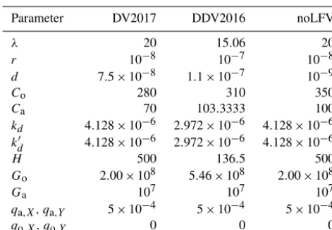
∂x. (42) In the same spirit, we consider the atmospheric variables out-side of this invariant manifold to be unresolved, all the other variables being resolved. The modesF2, F3, F4, F7 andF8 are outside of this invariant set, and therefore the variables ψa,2, ψa,3, ψa,4, ψa,7, ψa,8, θa,2, θa,3, θa,4, θa,7, θa,8 are considered as unresolved. Using the same parameteriza-tions, parameters and methods as in Demaeyer and Vannit-sem (2017), we should recover the same results with our cur-rent implementation5. This would thus provide a first manda-tory check for the correctness of the current implementation. We show the results obtained in Fig. 2 for the DV2017 pa-rameter set, where the probability density functions (PDFs) of three important variables of the dynamics are displayed. These three variables areψa,1,ψo,2andθo,2, and they were shown in Vannitsem and Ghil (2017) to account for respec-tively 18 %, 42 % and 51 % of the variance in some key reanalysis two-dimensional fields over the North Atlantic Ocean. In Vannitsem et al. (2015), it was also shown that these three variables are dominant in the LFV pattern found in the VDDG model version of MAOOAM. In addition to the PDFs of the full coupled system (13) and of the uncoupled systemX˙ =FX(X), the PDFs of the parameterizations are depicted in Fig. 2 with two different settings for the correla-tion and covariance matrices. Indeed, the two methods need the specification of the correlation and covariance matrices of the unresolved dynamics (34). These are the matricesσY; 6 and tensor 62 for the MTV method (see Appendix A); and the matricesσY, Y⊗Ysρ
0,Y and tensors ρ∂Y,ρY ∂Y Y for the WL method (see Appendix B). In the present case, with a parameterization based on the invariant manifold, the dynamics of the unresolved system (34) is a multidimen-sional Ornstein–Uhlenbeck process, for which the measure 5The code used in Demaeyer and Vannitsem (2017) is different
(a) (b)
(c)
Figure 2.Probability density functions (PDFs) of the dominant variables of the system dynamics with the invariant manifold decomposition for the XandY components. The densities of the full coupled system (13) and of the uncoupled system are depicted for the DV2017 parameter set, as well as the ones of the MTV and WL parameterizations and their verifications. The “check” label indicates that the correlations used for the parameterizations were analytical, while for the others they were obtained by numerical analysis.
Table 2.Component averaged Kullback–Leibler divergence with respect to the distributions of the full coupled system, in the case of the wavenumber 2 atmospheric variables parameterization. The abbreviations “atm.” and “oc.” refer to atmospheric and oceanic variables.
Barotropic atm. Baroclinic atm. Barotropic oc. Temperature oc.
Uncoupled MTV Uncoupled MTV Uncoupled MTV Uncoupled MTV
DDV2016 0.3343 0.0075 0.1643 0.0066 0.4592 0.0811 0.8148 0.0346
DV2017 0.0776 0.0022 0.0476 0.0031 0.1477 0.0822 0.1886 0.0379
(a) (b)
(c)
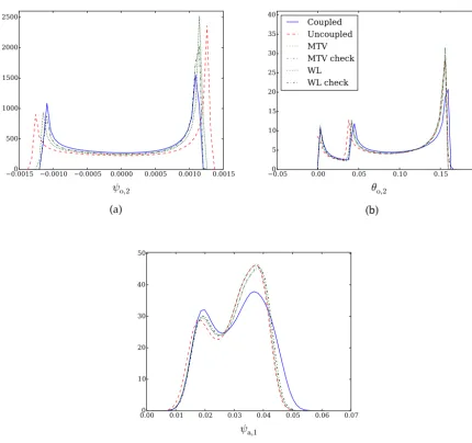
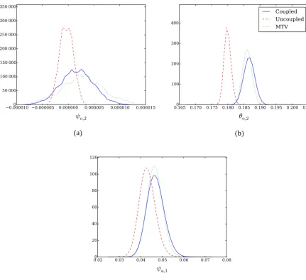
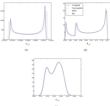
Figure 3.Probability density functions (PDFs) of the dominant variables of the system dynamics as in Fig. 2, but for the wavenumber 2 parameterization and with the parameter set DDV2016. The WL parameterization results are not shown as it is unstable and diverges.
is well known and thus analytical expressions for the corre-lations can be provided to the code. This analytical solution is also used in Demaeyer and Vannitsem (2017) and is one of the settings that we used to compute the parameterization. This setting is also compared with a setting using a numeri-cal least-squares regression method to obtain the correlation of variables of the system (34), assuming that these are of the simplified form
aexp
−t τ
cos(ωt+k), (43)
wheret is the time lag andτ is the decorrelation time. The results obtained for these two different settings of the cor-relation (analytical vs. numerical) are shown in Fig. 2 with “check” indicating the results obtained with the analytical ex-pressions for the correlations. The latter exex-pressions improve the correction of the dynamics for both the WL and the MTV
methods and we recover the same results as in Demaeyer and Vannitsem (2017).6On the other hand, in the case where the correlations are specified by the results of the numerical anal-ysis, the parameterizations perform less well, indicating that these methods can be very sensitive to a correct representa-tion of the correlarepresenta-tion structure of the unresolved dynamics.
Both the MTV and the WL methods correct the oceanic variables better, whereas the atmospheric variables seem to display very different dynamical behaviors between the cou-pled and uncoucou-pled systems which are difficult to correct. As stated in Demaeyer and Vannitsem (2017), it may be due to the huge dimension of the unresolved system, with half of the atmospheric mode being parameterized. However, the
6In fact, for the present parameterization based on the invariant
(a) Correlation function of . (b) Correlation function of .
(c) Correlation function of . (d) Correlation function of .
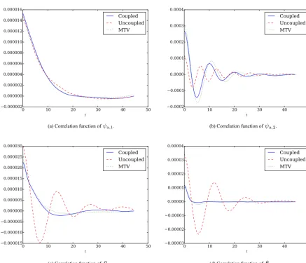
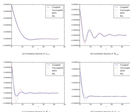
Figure 4. Correlation function of various variables for the wavenumber 2 parameterization and with the parameter set DDV2016. The correlation of the full coupled system (13), the uncoupled system and the MTV parameterizations are depicted as a function of the time lagt
(in days). The WL parameterization results are not shown as it is unstable and diverges.
decomposition based on the invariant manifold is an elegant one, based on deep properties of the advection operator (42). It leads to simplified coupling and is thus computationally advantageous. Within this framework, an adaptation based on the next order of both parameterization methods or the consideration of other parameterizations could lead to a very efficient correction for both the ocean and atmosphere.
As the present implementation allows for an arbitrary se-lection of the resolved–unresolved components, we shall now consider cases of the VDDG model version with dif-ferent unresolved components.
4.1.2 Parameterization of the wavenumber 2 atmospheric variables
We consider now a smaller set of unresolved variablesY, composed of the two higher-resolution modes of the model:
F9(x0, y0) = 2 cos(2nx0)sin(2y0), F10(x0, y0) = 2 sin(2nx0)sin(2y0).
(44) The unresolved variablesY are thus the following ones: ψa,9,ψa,10,θa,9andθa,10.
in-(a) (b)
(c)
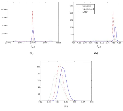
Figure 5.Probability density functions (PDFs) of the dominant variables of the system dynamics as in Fig. 2, but for the wavenumber 2 parameterization and with the parameter set “noLFV”. The WL parameterization results are not shown as it is unstable and diverges.
stabilities were still present, leading us to suspect a genuine instability in the parameterized system. Indeed, we found that it is the cubic termM(s)in the memory termM3 (see Eq. B30) which causes the divergence, in particular the in-teractions with theF4mode. These cubic terms are nonlinear dampings, as shown in Majda et al. (2009) and Peavoy et al. (2015). On the contrary, the MTV parameterization is sta-ble and performs well, despite having a similar cubic term. It indicates that the correlations induced by the memory term are a possible cause of the instability. More research effort to understand this stability issue is needed.
The quality of the solutions obtained with the MTV method alone, applied to the system with the three param-eter sets of Table 1, is evaluated using the Kullback–Leibler divergence
DKL(pkq)=
∞ Z
−∞
dxlogp(x)
q(x) (45)
stream-(a) Correlation function of . (b) Correlation function of .
(c) Correlation function of . (d) Correlation function of .
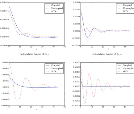
Figure 6.Correlation function of various variables for the wavenumber 2 parameterization and with the parameter set noLFV. The correlation of the full coupled system (13), the uncoupled system and the MTV parameterizations are depicted as a function of the time lagt(in days). The WL parameterization results are not shown as it is unstable and diverges.
Table 3.Component averaged Kullback–Leibler divergence with respect to the distributions of the full coupled system, in the case of the wavenumber 2 atmospheric baroclinic variables’ parameterization.
Barotropic atm. Baroclinic atm. Barotropic oc. Temperature oc.
Uncoupled MTV WL Uncoupled MTV WL Uncoupled MTV WL Uncoupled MTV WL
DDV2016 0.0097 0.0352 0.0104 0.0104 0.0145 0.0032 0.1983 0.0932 0.1120 0.1191 0.0700 0.0930
DV2017 0.0110 0.0036 0.0016 0.0018 0.0013 0.0003 0.1312 0.0781 0.0227 0.1277 0.0152 0.0090
noLFV 0.0208 0.1070 0.0433 0.0233 0.0660 0.0174 0.1891 0.0597 0.0523 0.1041 0.3696 0.0998
function) that gets better corrected, while on the contrary, in the ocean, it is the temperature field which benefits the most from the parameterization effects.
As depicted in Figs. 3 and 5, the PDFs of the three dom-inant variables selected show a neat correction, with a good representation of the LFV when it is present, and a correct shift in the dynamics and the temperature when no LFV oc-curs. In particular, one can notice in Fig. 3 a change in the
(a) (b)
(c)
Figure 7.Probability density functions (PDFs) of the dominant variables of the system dynamics as in Fig. 2, but for the wavenumber 2 parameterization. It is shown for the parameter set noLFV but with the wind stress parameter set tod=0.5×10⁻⁹and for which the MTV parameterization depicts a false LFV.
With this change in parameter, the system now lies near the Hopf bifurcation generating the long periodic orbit which forms the backbone of the LFV. In other words, the system does not exhibit a LFV but a small parameter perturbation could induce it. As seen in Fig. 7, the MTV parameterization then induces a LFV which is not present in both the resolved and the full system. In that case, the parameterization wrong-fully triggers a bifurcation and thus leads to a false reduced dynamics. This interesting issue, also considered by recent works on the effect of the noise on model dynamics, will be further discussed in the conclusion of this paper (see Sect. 5). The impact of the MTV parameterization on the correla-tion is also particularly important, as seen in Figs. 4 and 6, correcting the covariance (the value at the time lagt=0) and inducing or suppressing oscillations. It shows that the
param-eterization not only affects the attractors and the climatolo-gies of the models, but also the temporal dynamics.
Additional marginal PDF and autocorrelation function fig-ures are available for each variable of the system in the Sup-plement. The Kullback–Leibler divergences (45) are avail-able as well.
Since the WL parameterization does not work in the cur-rent case, we cannot properly compare both methods. To do so, we shall consider two other parameterization configura-tions in the following secconfigura-tions.
4.1.3 Parameterization of the wavenumber 2 atmospheric baroclinic variables
(a) (b)
(c)
Figure 8.Probability density functions (PDFs) of the dominant variables of the system dynamics as in Fig. 2, but for the wavenumber 2 baroclinic parameterization and with the parameter set DV2017.
Table 4.Component averaged Kullback–Leibler divergence with respect to the distributions of the full coupled system, in the case of the wavenumber 2 andF4modes atmospheric parameterization.
Barotropic atm. Baroclinic atm. Barotropic oc. Temperature oc.
Uncoupled MTV WL Uncoupled MTV WL Uncoupled MTV WL Uncoupled MTV WL
DV2017 0.1409 0.0376 0.0087 0.1910 0.0252 0.0042 1.1779 0.1254 0.2035 1.4277 0.0613 0.1369
noLFV 0.6905 1.1874 0.3076 0.4360 1.0114 0.1578 0.0214 0.1337 0.2368 1.2016 1.1374 0.8179
the comparison of the WL and the MTV methods. Indeed, in this configuration, the destabilizing cubic interactions with the modeF4are suppressed and the WL parameterization is now stable. The results are summarized in Table 3 where the Kullback–Leibler divergence (45) of the parameterizations’ marginal distributions with respect to the full coupled system ones are indicated. The divergence of the uncoupled system
(a) Correlation function of . (b) Correlation function of .
(c) Correlation function of . (d) Correlation function of .
Figure 9.Correlation function of various variables for the wavenumber 2 parameterization and with the parameter set DV2017. The corre-lation of the full coupled system (13), the uncoupled system, and the MTV and the WL parameterizations are depicted as a function of the time lagt(in days).
– The parameterizations correct quite well the ocean com-ponents, except for the MTV parameterization of the baroclinic component in the noLFV case. The MTV pa-rameterization is better in the DDV2016 case, and the WL one is better in the two other cases.
– The barotropic component of the atmosphere is only well corrected in the DV2017 case. Additionally, the MTV fails to correct also the baroclinic PDFs in the two other cases. In fact, the MTV method seems to only perform well in the DV2017 case. Looking to the divergence for every variable (see the Supplement), we note that those underperformances are due to the incorrect representation of the small-scale wavenum-ber 2 barotropic variables, namely theψa,6–ψa,10(ψa,5– ψa,10) variables for the WL (MTV) method.
Interestingly, the PDFs of the dominant variables ψa,1, ψo,2 andθo,2are well corrected as shown in Fig. 8 for the
DV2017 case and slightly better corrected in Fig. 10 for the DDV2016 case. We remark that in general the WL parame-terization is better at correcting the LFV than the MTV one, but the situation can be more complicated, like in Fig. 10b, where the WL parameterization captures one mode of the distribution well, and the MTV parameterization captures an-other mode well.
(a) (b)
(c)
Figure 10.Probability density functions (PDFs) of the dominant variables of the system dynamics as in Fig. 2, but for the wavenumber 2 baroclinic parameterization and with the parameter set DDV2016.
It also may explain the poor scores of the atmospheric zonal wavenumber 2 modes noted above. It implies that by param-eterizing baroclinic variables at certain scales, one should not expect these methods to perform well for the barotropic vari-ables at the same scale.
4.1.4 The parameterization of the atmospheric wavenumber 2 andF4modes
Another possibility to test the WL parameterization is to re-move the aforementioned cubic interactions by considering that the wavenumber 2 modes and the meridional mode F4(x0, y0)=
√
2 cos(2y0) (46)
are unresolved. In this case the variables ψa,4, θa,4,ψa,9, ψa,10,θa,9andθa,10 are considered as unresolved. The WL
method is then stable and this configuration allows us to com-pare both parameterizations.
(a) (b)
(c)
Figure 11.Probability density functions (PDFs) of the dominant variables of the system dynamics as in Fig. 2, but for the wavenumber 2 andF4modes parameterization and with the parameter set DV2017.
The PDFs of the three main variables (see Fig. 11) show that both parameterizations induce a change in modality for ψa,1 and a good correction of the LFV. We note that the MTV method corrects better the LFV signal in the dominant oceanic modesψo,2andθo,2(as also shown in Table 4). 4.2 The 5×5 model version
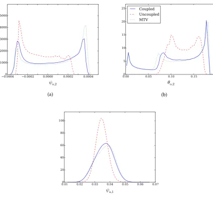
A higher-resolution test with the MTV method has also been performed by considering the 5×5 resolution system dis-cussed at Sect. 4. In this version, the resolution goes up to wavenumber 5 in every spatial direction and in every compo-nent. We do a quite drastic reduction of the dimensionality of the system by considering every mode above the wavenum-ber 2 in the atmosphere as unresolved. Consequently, the uncoupled system is an “atm-2x-2y oc-5x-5y” model
(a) (b)
(c)
Figure 12.Parameterization of the 5×5 model version with the MTV parameterization.(a)Two-dimensional probability density function (PDF) of the fully coupled dynamics with respect to the two dominant oceanic modes.(b)Anomaly of the PDF of the uncoupled dynamics with respect to the fully coupled one.(c)Anomaly of the PDF of the MTV dynamics with respect to the fully coupled one.
then it calls for even-higher-resolution tests for confirmation. Finally, the parameterization may genuinely well correct the ocean while having trouble with improving the atmosphere representation, for instance with the invariant manifold pa-rameterization described in Sect. 4.1.1 (see Fig. 2c).
5 Conclusions
In the present work, we have introduced a new framework to test different stochastic parameterization methods in the context of the ocean–atmosphere coupled model MAOOAM. We have implemented two methods: (i) a homogenization method based on the singular perturbation of Markovian op-erators and known as MTV (Majda et al., 2001; Franzke et al., 2005) (ii) and a method based on Ruelle’s response the-ory (Wouters and Lucarini, 2012), abbreviated as WL. The
code of the program is available in the Supplement, which allows for the future implementation of other parameteriza-tion methods in the context of a simplified ocean–atmosphere coupled model.
variables, even in the cases where a LFV is developing in the model. However, we have also found that the WL method shows instabilities, due to the cubic interactions therein. It indicates that the applicability of this method may crucially depend on the long-term correlations in the underlying sys-tem. The MTV method does not exhibit this kind of problem. Additionally, we have found that these methods are able to change correctly the modality of the distributions in some cases. However, in some other cases, they can also trigger a LFV that is absent from the full system. This leads us to underline the profound impact that a stochastic parameter-ization, and noise in general, can have on models. For in-stance, Kwasniok (2014) has shown that the noise can influ-ence the persistinflu-ence of dynamical regimes and can thus have a nontrivial impact on the PDFs, whose origin is the modifi-cation of the dynamical structures by the noise. In the present study as well, the perturbation of the dynamical structures by the noise is a very plausible explanation for the observed change in modality and for the good performances of the pa-rameterizations in general. However, if these perturbations can lead to a correct representation of the full dynamics, they can also generate regimes that are not originally present. This may happen near a bifurcation, as it is the case with the de-velopment of a wrong LFV regime, which develops around a long-period periodic orbit (Vannitsem et al., 2015) arising through a Hopf bifurcation. If the main parameter (here for instance the wind stress parameter d) is set close to this bi-furcation, the noise may thus trigger it while it is not present in the full system (Horsthemke and Lefever, 1984).
The MTV parameterization has also been tested in an intermediate-order version of the model, showing that this parameterization reduces the anomaly of the PDF of the two dominant oceanic modes. The atmospheric modes are how-ever less well corrected. In this case the number of modes that are removed is large and one can wonder whether reduc-ing this number or increasreduc-ing the resolution will help. More work needs to be done to assess the impact of the parameteri-zations on a higher-order version of the models in the future. The MTV method is simpler, less involved than the WL one, with no memory term estimations needed, and thus no integrals are being computed at every step. The memory term could however be Markovianized as in Wouters et al. (2016). The interest of the WL method is that it requires only a weak coupling between the resolved and the unresolved compo-nents, but no timescale separation between them, which is a desirable feature for a parameterization. Consequently, an improvement of the present framework would be to make the MTV method less dependent on the timescale separa-tion. One way to do that is to consider the next order inδ, the timescale separation parameter. This can be done effec-tively using the so-called Edgeworth expansion formalism, as shown by Wouters and Gottwald (2017). A next step would thus be to compute this expansion for the present coupled ocean–atmosphere system.
Finally, it would be interesting to consider that the unre-solved dynamics used to perform the averaging may have non-Gaussian statistics. In the present work, as stated in Ap-pendix A, the statistics of the neglected variables are as-sumed to come from a Gaussian distribution. However, de-pending on the terms regrouped in this discarded part of the system, the statistics may well be non-Gaussian, and the resulting parameterization developed in this Appendix is then only an approximation. Indeed, unresolved variables with different linear damping terms can lead to such non-Gaussianity (see Sardeshmukh and Penland, 2015). An ex-ample of it is the MTV parameterization of the wavenum-ber 2 in the 36-variable system (see Sect. 4.1.2), where the statistics are weakly non-Gaussian, because the linear damp-ing of the baroclinic unresolved variables is not the same as the barotropic ones. But other configurations are concerned as well. Taking this into account could probably improve fur-ther the results obtained in the present study.
Appendix A: The MTV method
We now consider Eqs. (23)–(24) and assume that the dynam-ics induced by the order 1/δ2term of theYdynamics can be replaced by (or behaves like) a multidimensional Ornstein– Uhlenbeck process:
˙ Y = 1
δ2A·Y+ 1
δBY·dWY, (A1) whereWY is a vector of independent Wiener processes. This dynamics thus generates Gaussian distributions, such that the odd-order moments vanish and that the even-order moments are related to the second-order one. This assumption is de-scribed in Majda et al. (2001) as a working assumption for stochastic modeling. It is related to other underlying assump-tions; i.e., that the dynamics of this singular term
˙ Y = 1
δ2FY(Y) (A2) is ergodic and mixing with an integrable decay of correla-tion (Franzke et al., 2005). In this case, the singular pertur-bation theory mentioned in Sect. 3.1.2 gives the following result (see Papanicolaou, 1976) in the limitδ1 for the pa-rameterization of the resolved component:
˙
X=FX(X)+R(X)+G(X)+ √
2σ(X)·dW, (A3) where
R(X)=1 δ
D
9X(X,Y)
E
e ρY
, (A4)
G(X)= 1 δ2
∞ Z
0
dsD9Y(X,Y)·∂Y9X(X,Ys)
E e ρY + 1 δ2 ∞ Z 0
dsD9X(X,Y)·∂X9X(X,Ys)
E
e ρY
, (A5)
and
σ2(X)=P(X), (A6)
with
P(X)= 1 δ2
∞ Z
0
dsD9¯X(X,Y)⊗ ¯9X(X,Ys)
E
e ρY
, (A7)
¯
9X(X,Y)=9X(X,Y)−
D
9X(X,Y)
E
e ρY
, (A8) and whereW is a vector of independent Wiener processes. Note that the termsG(X)andP(X)are of orderO(1), since the integrals over the lag timesin Eqs. (A5) and (A7) are of order7O(δ2). On the other hand, the termR(X)is of order
7It is due to the fact that we use directly the measure e
ρY of the
O(1/δ2)dynamics (A2) to perform the averaging, and not the mea-sure of the dynamicsY˙ =FY(Y).
O(1/δ)and identifies with the first term of the left-hand side of Eq. (A25) (see below).
The measureeρY is the one of the system (A2) or the mea-sure of the Ornstein–Uhlenbeck process (A1) replacing it. Similarly, Ys=φsY(Y)is the result of the evolution of the flowφYs of the system (A2) or the non-stationary solution of the Ornstein–Uhlenbeck process:
Ys=exp(As/δ2)·Y
+1 δ
s
Z
0
exp[A(s−τ )/δ2] ·BY·dWY(τ ). (A9)
In Sect. A1, we sketch the derivation of Eq. (A3), assum-ing that theY dynamics is an Ornstein–Uhlenbeck process. Furthermore, if the Y dynamics is an Ornstein–Uhlenbeck process like Eq. (A1), the results (A3)–(A7) can also be ex-panded to give a formula in terms of the covariance and cor-relation matrices of this process. Therefore, assuming that the dynamics of system (A2) has Gaussian statistics, its mea-sure can be used aseρYand these formula for the process (A1) can then be applied directly using the covariance and corre-lation matrices of system (A2). It gives a way to practically implement the parameterization as we detail it in Sect. A2. A1 Brief sketch of the parameterization derivation As stated in Sect. 3.1, the MTV parameterization is based on the singular perturbation theory of Markovian opera-tors. We follow the derivation proposed in Majda et al. (2001) and assume that the singular O(1/δ2) term is an Ornstein–Uhlenbeck process like Eq. (A1). The backward Kolmogorov equation for Eqs. (23)–(24) for the probability densityρδ(s,X,Y|t ), wheretis the final time, reads −∂ρ
δ
∂s =
1
δ2L1+ 1
δL2+L3
ρδ, (A10)
with the final condition given by some function ofX: ρδ(t,X,Y|t )=f (X).
The operators appearing in Eq. (A10) are given by L1=YT·AT·∂Y+δ
2BY :∂Y⊗∂Y, (A11)
L2=
YT·LXX T+BXXY :X⊗Y+BXY Y :Y⊗Y·∂X +XT·LY X T+YT ·LY Y T+BY XX:X⊗X
+BY XY :X⊗Y·∂Y, (A12)
L3=
HX+XT·LXX T+BXXX:X⊗X·∂X, (A13) whereT denotes the matrix transpose operation. Sinceδ 1, we can now perform an expansion procedure
and recast it in Eq. (A10), equating term by term at each or-der, to get
L1ρ0=0, (A14)
L1ρ1= −L2ρ0, (A15)
L1ρ2= − ∂ρ0
∂s −L3ρ0−L2ρ1. (A16)
The solvability condition for theses equations is that the right-hand side belongs to the range ofL1and thus that their average with respect to the invariant measure of Eq. (A1) vanishes. The first solvability condition is obviously satisfied but the second one is not necessarily satisfied since
PL2ρ0=
BXY Y :
D
Y⊗YE e ρY
·∂Xρ0=
BXY Y :σY
·∂Xρ0,
wherePis the expectation with respect to the measure of the process (A1) andσY is its covariance matrix. If the matrixA in Eq. (A1) is considered to be diagonal, as in Majda et al. (2001) and in Franzke et al. (2005), then it is satisfied. In-deed, in this caseσY is diagonal andPL2ρ0=0 due to the following property of the quadratic terms in the model:
∂ ∂Yi
BY Y Yi j k YjYk=0 .
However, here we do consider the general case:Ais not diag-onal and thus we can havePL2ρ06=0. It then indicates that 1/δeffects have to be taken into account in the parameteriza-tion. This can be done by following the method to treat “fast-waves” effects described in Majda et al. (2001). From here we thus depart from the standard derivation, to include those 1/δ effects in the parameterization. We need to assume that two timescales are present in the parameterization and con-sider them in the Kolmogorov Eq. (A10). Hence, we modify it explicitly by setting
∂ ∂s → ∂ ∂s+ 1 δ ∂ ∂τ and
ρδ(s, τ,X,Y|t )=ρ0(s, τ,X,Y|t )+δ ρ1(s, τ,X,Y|t ) +δ2ρ2(s, τ,X,Y|t ) .
Again, recasting this expansion in Eq. (A10) and equating term by term at each order, we obtain
L1ρ0=0, (A17)
L1ρ1= −L2ρ0−∂ρ0
∂τ , (A18)
L1ρ2= − ∂ρ0
∂s − ∂ρ1
∂τ −L3ρ0−L2ρ1. (A19) The solvability condition of Eq. (A17) imposes thatPL1ρ0= 0. SincePL1ρ0=PL1Pρ0=0, it means thatPρ0=ρ0and
that ρ0 belongs to the null space ofL1. As a result of the introduction of the 1/δtimescale in the equations, the second solvability conditionPL1ρ1=0 is now tractable and gives ∂ρ0
∂τ = −PL2Pρ0, (A20)
and thus ρ1= −L−11
L2ρ0+∂ρ0 ∂τ
. (A21)
These two equations give together
ρ1= −L−11 L2ρ0−PL2Pρ0. (A22) SincePcommutes withL−11and sincePP=P, we thus have thatPρ1=0 andP∂ρ1/∂τ=0. The solvability condition of Eq. (A19) imposes thatPL1ρ2=0 and thus
−P∂ρ0 ∂s =P
∂ρ1
∂τ +PL3Pρ0+PL2ρ1, (A23) which becomes, with Eq. (A22),
−∂ρ0
∂s =PL3Pρ0−PL2L
−1
1 L2−PL2
Pρ0. (A24) Finally, grouping Eqs. (A20) and (A24) together gives
− ∂ ∂s+ 1 δ ∂ ∂τ
ρ0=
1
δPL2P+PL3P−PL2L
−1
1 L2−PL2
P
ρ0, (A25) which is the result that was obtained in Papanicolaou (1976). From here, the computation proceeds along the standard line described in Majda et al. (2001) and gives the result (A3). A2 Practical implementation
We will now derive explicitly the MTV parameterization for the system (27)–(28). For the time of the derivation, we will again assume that theY dynamics is given by the pro-cess (A1), but we suppose that the final results apply as well with the measure, covariance and correlation matrices of sys-tem (A2).
We consider first the case defined by Eq. (35) where the intrinsic dynamics is considered to be given by the quadratic terms of the tendencies alone. We define the matrix
6=
∞ Z
0
dsDY⊗YsE e ρY
(A26)
and we note that
∞ Z
0
dsD∂Y⊗YsE e ρY
D
Y⊗∂Y⊗YsE e ρY
=0, (A28)
D
∂Y⊗Ys⊗Ys
E
e ρY
=0, (A29)
∞ Z
0
dsDYi∂YjY s kY s l E e ρY = ∞ Z 0 ds NY X
m=1 σj m−1
D
YmYks
E
e ρY
D
YiYls
E
e ρY
+DYmYls
E
e ρY
D
YiYks
E
e ρY
, (A30)
sinceDYsE e ρY
=0 and whereσY is the covariance matrix of the process (A1). These results can be explicitly obtained us-ing the non-stationary solution (A9). We also define
62=
∞ Z
0 ds
D
Y⊗YsE e ρY
⊗DY⊗YsE e ρY
, (A31)
which is thus a rank-4 tensor. Note that both6and62 are O(δ2)objects. With those definitions, it can be shown that the parameterization (A3) becomes
˙
X=FX(X)+R(X)+G(X)+ √
2σ(1)(X)·dW(1) +
√
2σ(2)·dW(2), (A32)
withDdW(1)(t )⊗dW(2)(t0)
E
=0 and
R(X)=1 δH
(3), (A33)
G(X)= 1 δ2
" 2 X
i=0 H(i)+
3
X
i=0 L(i)
!
·X
+B(1)+B(2):X⊗X+M: ·X⊗X⊗Xi, (A34) σ(1)(X)·hσ(1)(X)iT =P1(X)=
1 δ2
h
Q(1)+U·X+V:X⊗Xi, (A35) σ(2)·
h
σ(2)iT =P2= 1 δ2Q
(2). (A36)
The product “: ·” is similar to the definition (31) but with a rank-4 tensor and three variables:
M : ·X⊗X⊗X= NX
X
j,k,l=1
Mij klXjXkXl. (A37)
All the products involved concern the last and the first indices of respectively their first and second arguments. M andV are rank-4 tensors, Uis a rank-3 tensor and the Q(i)’s are matrices. TheH(i)’s are vectors, theL(i)’s are matrices and theB(i)’s are rank-3 tensors. The formula of these quantities are given below:
Hi(0)=LXYi ·σ−Y1·6T ·HY =
NY
X
j,k,l=1
LXYi j 6j kT σY−1 klH
Y
l , (A38)
Hi(1)=BXXYi :
LXY·6
=
NX
X
j=1 NY
X
k,l=1
BXXYi j k LXYj l 6lk, (A39)
Hi(2)=
BXY Yi +BXY Yi T⊗LY Yoσ−Y1·62
=
NY
X
j,k,l,m,n=1
BXY Yi j k +BXY Yi k j
LY Yl m
σY−1
j n(62)nlkm, (A40)
Hi(3)=BXY Yi :σY = NY
X
j,k=1
BXY Yi j k (σY)j k, (A41)
L(ij0)=BXXYi j ·
σ−Y1·6T ·HY = NY
X
k,l,m=1
BXXYi j k 6klTσY−1 lmH
Y
m, (A42)
Lij(1)=LXYi ·σY−1·6T ·LY Xj = NY
X
k,l,m=1
LXYi k 6TklσY−1 lmL
Y X
m j, (A43)
L(ij2)=BXY Yi +BXY Yi T⊗BY XYj oσ−Y1·62
=
NY
X
k,l,m,n,p=1
BXY Yi k l +B XY Y i l k
Bm j nY XY
σY−1
kp(62)pmln, (A44)
L(ij3)=BXXYi :BXXYj ·6= NX
X
k=1 NY
X
l,m=1
BXXYi k l BXXYk j m6ml, (A45)
Bij k(1)=LXYi ·
σ−Y1·6T ·BY XXj k = NY
X
l,m,n=1
LXYi l 6lmT σY−1 mnB
Y XX
n j k , (A46)
Bij k(2)=BXXYi j ·σY−1·6T ·LY Xk = NY
X
l,m,n=1
BXXYi j l 6TlmσY−1 mnL
Y X
n k, (A47)
Mij kl=BXXYi j ·
σ−Y1·6T ·BY XXk l = NY
X
m,n,p=1
BXXYi j m6mnT σY−1 npB
Y XX
p k l, (A48)
Q(ij1)=LXYi ·6·LXYj T = NY
X
k,l=1
LXYi k 6klLXYj l , (A49)
NY
X
k,l,m,n=1
BXY Yi k l BXY Yj m n+Bj n mXY Y(62)kmln, (A50) Uij k=LXYi ·6·BXXYj k +BXXYi j ·6·LXYk =
NY
X
l,m=1
LXYi l 6lmBXXYj k m+ NY
X
l,m=1
BXXYi j l 6lmLXYk m, (A51) Vj ikl=BXXYi k ·6·BXXYj l =
NY
X
m,n=1
BXXYi k m6mnBj l nXXY, (A52)
where·is the product and summation over the last and the first indices of respectively its first and second arguments8. The product :is defined as in Eq. (31). The tensors whose indices are indicated define a lower rank tensor; for instance, the rank-3 tensorBXXY
i hence noted defines a matrix whose noted defines a matrix whose elements areBXXYi j k. The sym-bolothen defines the following permuted product and sum-mation of two given rank-4 tensorsCandD:
CoD=X ij kl
Cij klDikj l. (A53)
With the notable exception ofH(0),H(3)andL(0), one can easily check that the formulation (A39)–(A52) gives back the formulas of the Appendix in Franzke et al. (2005) whenσY is diagonal. It is these particular tensors that are implemented and computed by the code provided with the present article as Supplement. They are computed using the covariance ma-trixσY and the integrated correlation matrices6and62as input. The formulas presented here are valid for an Ornstein– Uhlenbeck process, but as stated above, the covariance and correlations of the dynamics (A2) can be used directly as well, provided that the right assumptions are fulfilled. In the present work, we have always used the statistic of Eq. (A2) to compute the tensors. Once the tensors are available, the resulting tendencies are then computed at each time step and Eq. (A3) can be integrated with one of the available integra-tors.
This solves the case when the singular perturbation O(1/δ2)term is given by Eq. (35). In the case where the O(1/δ2)term is given by Eq. (34), i.e., the intrinsic dynam-ics, it is straightforward to show that the parameterization is exactly the same, except thatH(0)=H(2)=L(0)=0. A3 Technical details
The Eq. (A32) is integrated with a stochastic Heun algorithm described in Greiner et al. (1988) and which converges to-ward the Stratonovich statistic (Hansen and Penland, 2006). In particular, theR(X)andG(X)terms and theP1(X)and P2matrix are computed by performing sparse-matrix prod-ucts. The square root of the matrix P2 is computed once
8Thus, for vectors and matrices it is the standard product.
at initialization with a singular-value decomposition (SVD) method to obtain the matrixσ(2). The square root of the state-dependent matrixP1(X)is computed eachmnutitime9to obtain the matrixσ(1)(X), again with SVD. In general, in the present work, we have setmnutiequal to the Heun al-gorithm time step.
Appendix B: The WL method
The Wouters–Lucarini method is considered with the decom-position (34) and consists of three terms (Wouters and Lu-carini, 2012):
˙
X=FX(X)+ε M1(X)+ε2M2(X, t )+ε2M3(X, t ), (B1) which we detail now in the following.
B1 TheM1term
This is the averaging term, which is defined as M1(X)=D9X(X,Y)
E
ρ0,Y
, (B2)
whereρ0,Y is the measure of the unperturbed intrinsic dy-namics (34). Since
9X(X,Y)=LXY·Y+BXXY :X⊗Y+BXY Y :Y⊗Y, (B3) we get the following result:
M1(X)=LXY·µY +BXXY :X⊗µY+BXY Y :σY, (B4) whereµY =DYE
ρ0,Y
is the mean of the dynamics (34) andσY its covariance matrix. In the following, we shall assume that this dynamics is Gaussian; henceµY =0 and we get M1(X)=BXY Y :σY. (B5) B2 TheM2term
This is the correlation term, which here can be written as follows:
M2(X, t )=9X,0 1(X)T ·aXY·σ(t ) . (B6) Indeed, since9X0 (X,Y)=9X(X,Y)−M1(X),9X0 can be decomposed as a product of the Schauder basis function of XandY (Wouters and Lucarini, 2012):
9X0 (X,Y)= 2
X
i,j=1
9X,0 1,i(X)·ai jXY·9X,0 2,j(Y), (B7)
9The notationmnutiindicates a parameter of the code
with the basis
9X,0 1,1(X)=1, (B8) 9X,0 1,2(X)=XT, (B9) and
9X,0 2,1(Y)=Y−µY, (B10)
9X,0 2,2(Y)=vec(Y⊗Y−σY) . (B11) The notation vec denotes an operation stacking the columns of a matrix into a vector:
(vecA)I (i,j )=Aij with I (i, j )=div(j, n)+i, (B12) where div(a, b)is the integer division ofabybandnis the second dimension ofA. The vector vec(Y⊗Y−σY)is thus aNY2 length vector. The objectaXYij in Eq. (B7) can then be rewritten as a matrix:
aXY =
LXY mat BXY Y
BXXY 0
, (B13)
where we define
9X,0 1,1(X)·a1XYj =1·a1XYj =a1XYj
= LXY mat BXY Y, (B14)
and
XT·BXXY·Y=BXXY :X⊗Y. (B15) The notation mat denotes an operation transforming rank-3 tensors into matrices, e.g.,
matBXY Y iJ (j,k)
=BXY Yi j k with
J (j, k)=div(j, n)+k, (B16) wheren=NY is the second dimension ofBXY Y. With this notation, we have thus for instance
matBXY Y·vec(Y⊗Y)=BXY Y :Y⊗Y. (B17) Here, mat BXY Y
is thus aNX×NY2 matrix. The notations vec and mat introduced here are defined such that the ex-pression (B7) can now be written in the compact form with matrix products:
9X0 (X,Y)=9X,0 1(X)·aXYi j ·9X,0 2(Y). (B18) Now, the processσ(t )appearing in Eq. (B6) then has to be constructed (see Wouters and Lucarini, 2012) such that
D
σ(t )⊗σ(t+s)E=g(s), (B19) with
g(s)=D9X,0 2(Y)⊗9X,0 2(Ys)E ρ0,Y
(B20) =
g11(s) g12(s) g21(s) g22(s)
, (B21)
where g11(s)=
D
(Y−µY)⊗ Ys−µYE
ρ0,Y ,
g12(s)=
D
(Y−µY)⊗vec Ys⊗Ys−σY
E
ρ0,Y ,
g21(s)=Dvec(Y⊗Y−σY)⊗(Ys−µY)
E
ρ0,Y ,
g22(s)=
D
vec(Y⊗Y−σY)⊗vec Ys⊗Ys−σY
E
ρ0,Y ,
and whereYs=φYs(Y)is the result of the time evolution of the flow of the uncoupledY dynamics given by system (34). Now if we assume that this latter dynamics is Gaussian, the non-diagonal entries in the matrix above vanish, and we can write
σ(t )=
σ1(t ) vec(σ2(t ))
, (B22)
with
D
σ1(t )⊗σ1(t+s)
E
=DY⊗YsE ρ0,Y
−µY⊗µY, (B23)
D
σ1(t )⊗vec(σ2(t+s))E=0, (B24)
D
vec(σ2(t ))⊗vec(σ2(t+s))E=
D
vec(Y⊗Y)⊗vec Ys⊗YsE
ρ0,Y −Dvec(σY)⊗vec(σY)
E
ρ0,Y
, (B25)
whereσ2is aNY×NY matrix of processes. TheM2term can thus be written as follows:
M2(X, t )=LXY·σ1(t )+BXXY :X⊗σ1(t )
+BXY Y :σ2(t ). (B26)
B3 TheM3term
This is the memory term which is defined as
M3(X, t )=
∞ Z
0
ds h(X(t−s), s), (B27)
with h(X, s)=
D
9Y(X,Y)T ·∂Y9X(Xs,Ys)
E
ρ0,Y
(B28) =DLY X·X+BY XX:X⊗X+BY XY :X⊗YT
·∂YLXY·Y+BXXY :Xs⊗Y +BXY Y :Y⊗Y E
ρ0,Y
whereXs=φsX(X)is the result of the time evolution of the flow of the uncoupledXdynamics given by the systemX˙ = FX(X). Detailing each term in this expression,M3 can be rewritten as
M3(X, t )=
∞ Z
0
dshL(1)(s)+L(2)(s)·Xe
+B(1)(s):Xe⊗Xe+B(2)(s):eX⊗Xe
s +M(s): ·Xe⊗eX⊗Xe
si
e
X=X(t−s), (B30) witheX
s
=φXs (X(t−s))and L(ij1)(s)=LXYi ·ρ∂Y(s)T ·LY Xj =
X
k,l=1
LXYi k ρ∂Y(s)TklLY Xl j , (B31)
L(ij2)(s)=BY XYj T :ρY ∂Y Y(s):BXY Yi = NY
X
k,l,m,n=1
BY XYl j k ρY ∂Y Y(s)klmnBXY Yi mn, (B32) Bij k(1)(s)=LXYi ·ρ∂Y(s)T ·BY XXj k =
NY
X
l,m=1
LXYi l ρ∂Y(s)mlBm j kY XX, (B33)
Bij k(2)(s)=BXXYi j ·ρ∂Y(s)T ·LY Xk = NY
X
l,m=1
BXXYi j l ρ∂Y(s)mlLY Xmk, (B34) Mij kl(s)=BXXYi j ·ρ∂Y(s)T·BY XXk l =
NY
X
m,n=1
BXXYi j mρ∂Y(s)nmBY XXn k l , (B35)
since
D
Y⊗∂Y⊗Ys
E
ρ0,Y
=0, (B36)
D
∂Y⊗Ys⊗YsE ρ0,Y
=0, (B37)
because the dynamics of Eq. (34) is assumed to be Gaussian and where
ρ∂Y =
D
∂Y⊗YsE ρ0,Y
=σ−Y1·
D
Y⊗YsE ρ0,Y
, (B38)
ρY ∂Y Y=DY⊗∂Y⊗Ys⊗YsE ρ0,Y
, (B39)
and the expression of this last definition can be inferred from Eq. (A30).
B4 Technical details
The tendencies appearing in Eq. (B1) are computed accord-ing to the same Heun algorithm described in Sect. A3. A small difference with the latter here is that the termM3, due to its computational cost, is computed every mutitime10 and remains constant in between. The term M1 is simply obtained by computing sparse-matrix products. The process σ(t )of the termM2is emulated by a multidimensional nth-order autoregressive process (MAR(n)) described in Penny and Harrison (2007). The parameters and the ordernof this process can be assessed for instance by using the variational Bayesian approach described in this article. The integrand of the termM3 is obtained by computing sparse-matrix prod-ucts and integrating for each time step the uncoupledX dy-namics forward, to obtaineX
s
. The integral is then performed with a simple trapezoidal rule with a time stepmutiover a time interval which is set by the parametermeml. This inter-val should be set so that the absolute inter-value of the integrand has sufficiently decreased at the end of it. In practice, it is suf-ficient to setmemlproportional to the longest decorrelation time of the uncoupledY dynamics.
10The notationmutiindicates a parameter of the code