www.earth-syst-dynam.net/7/893/2016/ doi:10.5194/esd-7-893-2016
© Author(s) 2016. CC Attribution 3.0 License.
Assessing uncertainties in global cropland futures using
a conditional probabilistic modelling framework
Kerstin Engström1, Stefan Olin1, Mark D. A. Rounsevell2, Sara Brogaard3, Detlef P. van Vuuren4,5,
Peter Alexander2, Dave Murray-Rust6, and Almut Arneth7
1Department of Physical Geography and Ecosystem Science, Lund University, Sölvegatan 12,
22362 Lund, Sweden
2School of GeoSciences, University of Edinburgh, Geography Building, Drummond Street,
Edinburgh, EH89XP, UK
3Centre for Sustainability Studies, Lund University (LUCSUS), Biskopsgatan 5, 22362 Lund, Sweden 4PBL Netherlands Environmental Assessment Agency, Postbus 303, 3720 AH Bilthoven, the Netherlands
5Copernicus Institute for Sustainable Development, Faculty of Geosciences, Utrecht University,
Heidelberglaan 2, 3584 CS Utrecht, the Netherlands
6School of Informatics, University of Edinburgh Appleton Tower, 11 Crichton Street, Edinburgh, EH8 9LE, UK 7Karlsruhe Institute of Technology, Institute of Meteorology and Climate Research, Atmospheric
Environmental Research (IMK-IFU), Kreuzeckbahnstr. 19, 82467 Garmisch-Partenkirchen, Germany
Correspondence to:Stefan Olin (stefan.olin@nateko.lu.se)
Received: 25 February 2016 – Published in Earth Syst. Dynam. Discuss.: 15 March 2016 Revised: 16 August 2016 – Accepted: 6 September 2016 – Published: 17 November 2016
Abstract. We present a modelling framework to simulate probabilistic futures of global cropland areas that are conditional on the SSP (shared socio-economic pathway) scenarios. Simulations are based on the Parsimonious Land Use Model (PLUM) linked with the global dynamic vegetation model LPJ-GUESS (Lund–Potsdam–Jena General Ecosystem Simulator) using socio-economic data from the SSPs and climate data from the RCPs (rep-resentative concentration pathways). The simulated range of global cropland is 893–2380 Mha in 2100 (±1 standard deviation), with the main uncertainties arising from differences in the socio-economic conditions pre-scribed by the SSP scenarios and the assumptions that underpin the translation of qualitative SSP storylines into quantitative model input parameters. Uncertainties in the assumptions for population growth, technological change and cropland degradation were found to be the most important for global cropland, while uncertainty in food consumption had less influence on the results. The uncertainties arising from climate variability and the differences between climate change scenarios do not strongly affect the range of global cropland futures. Some overlap occurred across all of the conditional probabilistic futures, except for those based on SSP3. We conclude that completely different socio-economic and climate change futures, although sharing low to medium population development, can result in very similar cropland areas on the aggregated global scale.
1 Introduction
Land use and land cover change (LULCC) is a fundamen-tal aspect of global environmenfundamen-tal change, but large uncer-tainties exist in estimating the effect of multiple drivers on LULCC in the future (Brown et al., 2014). A range of dif-ferent models and scenarios have been used to project future
productivity (Schmitz et al., 2014; Smith et al., 2010). The direction of socio-economic drivers is referred to as deep un-certainties, which are addressed through the use of scenarios (van Vuuren et al., 2008). Cropland projections at the high end of the projected uncertainty range for global cropland would have profound consequences for, for example, global carbon and nitrogen fluxes, the global water balance, biodi-versity, and other ecosystem services (Lindeskog et al., 2013; Pereira et al., 2012; Zaehle et al., 2007). Hence, quantifying and understanding the inherent uncertainties in the drivers of LULCC has important consequences for policy responses to support sustainable development. However, the effects of un-certainties in the underlying scenario assumptions have not been systematically quantified for global cropland projec-tions.
Scenarios are characterized by storylines that describe as-sumptions about key drivers and processes from which model input parameters are interpreted (Rounsevell and Metzger, 2010). These parameter interpretations are by definition de-terministic within a scenario context, since they do not con-sider the uncertainties associated with the interpretation pro-cess itself. By contrast, probabilistic approaches examine system uncertainties by assigning probability distributions to input variables (reflecting uncertainties about scenario as-sumptions) to assess the influence of uncertainty on system outputs (van Vuuren et al., 2008). The conditional probabilis-tic approach combines the strength of scenarios in address-ing deep uncertainties with the probabilistic approach that explores the uncertainties in the assumptions about model in-put parameters (O’Neill, 2005; van Vuuren et al., 2008). In this case, the probability distribution of each model input pa-rameter is conditional on the internal logic and assumptions within the contextualizing scenario. Hence, conditional prob-abilistic futures are useful in exploring parameter uncertainty within and across scenarios (Brown et al., 2014; van Vuuren et al., 2008).
In this paper, we present probabilistic futures of global cropland that are conditional on scenario assumptions. In do-ing so, we quantify the uncertainties within these assump-tions, as well as representing the deep uncertainty across dif-ferent scenarios. The assessment is based on the following key questions:
– How will cropland area evolve until 2100 in response to socio-economic drivers and climate change?
– Will future ranges of global cropland for different sce-narios overlap due to differences in socio-economic conditions and/or due to uncertainties in model input parameters?
– How does the influence of the uncertainties in model input parameters change through time?
We use a scenario framework based on the five shared socio-economic pathways (SSPs) and develop a scenario
ma-trix combining the five SSPs and four representative con-centration pathways (RCPs). This scenario matrix is filled with probabilities based on the assumption that a given SSP will correspond to a given RCP. For each SSP, we derive RCP-specific input (yields in this case) applying the sce-nario matrix. The resulting conditional probabilistic futures are named F1–F5, where the numbers 1–5 correspond to SSP1–5. The RCP–SSP scenario framework was used since it is the most recent scenario approach for global environ-mental change research (Ebi et al., 2014; O’Neill et al., 2016; van Vuuren et al., 2011, 2014). We apply these sce-narios to a global-scale, socio-economic model of agricul-tural land use change (the Parsimonious Land Use Model, PLUM; Engström et al., 2016) in combination with crop yield time series derived from the dynamic global vegetation model, LPJ-GUESS (Lund–Potsdam–Jena General Ecosys-tem Simulator; Lindeskog et al., 2013; Smith et al., 2001). PLUM has been benchmarked against different models and scenario studies in a land use model intercomparison exercise (Alexander et al., 2016; Prestele et al., 2016) that has demon-strated its consistency in comparison with other global crop-land simulations. Because of its rapid runtimes, PLUM can explore uncertainties across its input parameter space (En-gström et al., 2016) and hence is appropriate for use in prob-abilistic simulations requiring multiple model iterations.
2 Materials and methods
2.1 Conditional probabilistic futures within the SSP–RCP scenario framework
To construct the conditional probabilistic futures (F1–F5) we used qualitative and quantitative information from the SSPs directly and quantitative information from the RCPs indi-rectly as input to PLUM (Fig. 1).
PLUM SSPs
SSPs SSPs
SSPs SSPs SSPs
SSPs SSPs
RCPs
LPJ‐GUESS Climate pattern RCPs
Yield for each RCP
Socio‐economic parameters: mean and standard deviation
Scenario matrix Yield for each SSP
Land use
futures Land use
futures Land use
futures Land use
futures Cropland
futures F1‐F5 GCMs
GCMs GCMs
GCMs GCMs
Figure 1. The SSP–RCP modelling framework. The RCPs and SSPs, as well as the scenario matrix (author judgement about the distribution of RCPs conditional on SSPs), are input to the model (indicated in blue). Models (indicated in orange; GCMs: general circulation models) use input or results of other models (intermedi-ate results, indic(intermedi-ated in green). The final outputs of the modelling framework are the cropland futures F1–F5 (indicated in red).
presents a great challenge for mitigation, but a small chal-lenge for adaptation. SSP4 presents a small chalchal-lenge for adaptation but a great challenge for mitigation because in-equality is high across and within countries, and various lev-els of economic and technological development benefit the global elite.
In the modelling framework presented here, the ent socio-economic pathways were combined with differ-ent levels of climate change associated with the four RCPs. The RCPs are defined by their forcing targets from 2.6 to 8.5 W m−2at the end of the 21st century and trajectories of emission changes (van Vuuren et al., 2011). The radiative forcing of the RCPs is likely to correspond to global mean temperature increases between 0.3 and 4.8◦C by the end of the 21st century (2081–2100) relative to the 1986–2005 global mean temperature (in the 5 to 95 % range; Collins et al., 2013). The impact of climate change on crop yields was estimated for all RCPs by running LPJ-GUESS with climate inputs derived from five different general circulation models (GCMs; Collins et al., 2011; Dufresne et al., 2013; Dunne et al., 2013; Iversen et al., 2013; Watanabe et al., 2011).
The SSPs and RCPs were combined within a scenario ma-trix to reflect assumptions about the plausibility of an RCP arising from an SSP. Theoretically, all cells within this ma-trix are possible, but not all combinations of SSPs and RCPs are equally plausible and consistent (van Vuuren and Carter, 2014; van Vuuren et al., 2014). For instance, van Vuuren et al. (2012) indicate that emissions are only likely to be as high as assumed under RCP8.5 with large-scale use of fossil fuels, driven either by rapid economic growth (and little substitu-tion towards less carbon-intensive fuels) or very high popula-tion growth. By contrast, for the matrix cells at the lower end
of the RCP range (2.6 and 4.5 W m−2), the SSPs would need to assume strong mitigation efforts, but this would be less plausible for the SSPs with great challenges to mitigation. Here, we use the SSPs as reference scenarios as described in O’Neill et al. (2016) without introducing any specific miti-gation policies (as could be done using the shared policy as-sumptions, SPAs; Kriegler et al., 2014). The SPAs define key attributes of climate policy, e.g. climate goals, policy regimes and measures (Kriegler et al., 2014). However, some SSP– RCP combinations remain unlikely either at the low or high end. Without the introduction of specific mitigation policies, the SSP–RCP combinations are referred to as reference sce-narios (O’Neill et al., 2016).
The conditional probabilistic approach was implemented through the following steps (van Vuuren et al., 2008):
1. identification of uncertain parameters;
2. estimation of the conditional probability ranges associ-ated with these parameters, i.e. their probability density functions (PDFs);
3. use of Monte Carlo sampling across the PDFs to under-take multiple simulations;
4. identification of the uncertainty ranges in model out-comes and the determinants of model uncertainty.
Thus, the uncertainty ranges of the global model output vari-ables arise from
a. uncertainties in the PLUM socio-economic input pa-rameters and
b. uncertainties in climatic variation and sampling from the scenario matrix for the crop yield simulations.
The effect of a. was explored in combination with b. for global output variables. We hypothesize that the effect of b. is smaller than the effect of a. on the range of global cropland change. This hypothesis was tested by undertaking model runs in which only the socio-economic parameter uncertain-ties were explored. This stepwise approach is described in more detail below (Sect. 2.3: steps 1–3 for a.; Sect. 2.4: steps 1–3 for b; Sect. 2.5: step 4).
2.2 PLUM simulations – descriptions of future cropland
PLUM simulates agricultural land use in terms of cropland for 1601 countries (Engström et al., 2016). The model is based on a simple demand and supply strategy, where de-mand of agricultural products is driven by population, eco-nomic development and dietary changes. The supply of agri-cultural products, indicated by cereals, is met by a simple
1The availability of input data determines the number of
trade mechanism, where all countries are assumed to have access to the global market. Changes in cropland are as-sumed to be proportional to changes in cereal land, apply-ing a constant country-specific cropland–cereal-land ratio derived from FAOSTAT data in the baseline year of 2000 (for a detailed description of PLUM, see Engström et al., 2016). Globally, cereal land alone accounted for 60 % of cropland in 2010 (FAOSTAT, 2015). PLUM can reproduce global his-toric agricultural land use change (1990–2010), and results have demonstrated that agricultural land use is highly sen-sitive to uncertainties in crop yield growth rates (Engström et al., 2016). To estimate the temporal trends and changes in spatial patterns of crop yields in response to climate change, country-level cereal yields were derived from the global dynamic vegetation model LPJ-GUESS (Lindeskog et al., 2013; Smith et al., 2001). LPJ-GUESS accounts for the ef-fects of temperature, precipitation and atmospheric CO2
con-centrations on crop yields and the productivity of natural veg-etation. It models the yields of 11 globally important crops, including wheat, maize and rice (Lindeskog et al., 2013), and also accounts for management options such as sowing and harvesting in response to climatic conditions.
To derive LPJ-GUESS country-level projections of actual and potential cereal yield, LPJ-GUESS simulations were per-formed on a 0.5◦ grid from 2000 until 2100 for four cereal crops (wheat, maize, millet/sorghum and rice), both rain fed and irrigated. To calculate the yearly actual yield per grid cell, the per grid cell share of irrigated vs. rain-fed area in the year 2000 was derived from the MIRCA (monthly irri-gated and rainfed crop areas) data set (Portmann et al., 2010) and applied over the entire simulation period. For potential yields, we chose the maximum of either rain-fed or irrigated yields in each grid cell where the crop was present in the MIRCA data set. Naturally in most cases irrigated yields are larger and less fluctuating. The per grid cell actual and poten-tial yields for the year 2000 were then scaled to the grid cell actual and potential yield from Mueller et al. (2012) in order to establish the difference (yield gap) between actual and po-tential yields. This scaling factor was then used for all years in the yield time series. The yield time series were then ag-gregated to the country level based on the area fractions from the MIRCA data set. These aggregated county level time se-ries of actual and potential yield were used to sample yield time series as input to PLUM (Sect. 2.4.3). In PLUM, the yield gap was modelled to change over time depending on three scenario parameters describing technological change (Fig. 2). These three parameters describe the strength of tech-nological change per se and the investment and distribution of yield-improving management practices (see Appendix A). The potential yield is not influenced by the technological change parameters. Thus, further increases in potential yields arising from crop breeding and improved agricultural man-agement practices are not included here (see Fischer et al., 2014, for a review).
Figure 2.Decreasing yield gap for Ukraine. The scenario parame-ters related to technological change determine how rapidly the yield gap decreases over time (the arrow only being symbolic, indicating the drivers of changing yield gap).
The country-level actual yields calculated in the previous step might differ slightly from the country statistics from FAOSTAT on which PLUM is based. Thus, as a final step, the yield calculated in PLUM was scaled to match yields re-ported in the year 2000 (FAOSTAT, 2015). The scaling factor for the year 2000 was applied throughout the simulation pe-riod. An example of the yield calculations is given in Fig. 2, for Ukraine. This example uses the socio-economic assump-tions from SSP5 and the yield projecassump-tions driven by RCP6.0. Carbon fertilization has a strong effect on crop yields; e.g. for Ukraine potential yields are simulated to increase from be-low 6 to above 8 t ha−1from 2000 to 2100 (dark grey dashed line, Fig. 2). Actual yield is simulated to increase by roughly 1 t ha−1 by the end of the 21st century (light grey dashed line, Fig. 2). However, the strong economic and technolog-ical change in SSP5 results in a tripling of yields during the period 2000–2100 (grey line, Fig. 2) and thus a decrease in the yield gap for Ukraine.
2.3 Uncertainties related to the socio-economic input parameters of PLUM
2.3.1 Identifying uncertain parameters in PLUM
Table 2.PLUM input parameter groups and the influence of SSP scenario elements (from O’Neill et al., 2016). In PLUM several of the input parameters were grouped together conceptually, as indicated by the parameter group number (no.). For example, there are four input parameters that describe meat consumption trajectories of different income and cultural groups (meat1–meat4, see Table 1), which all belong to meat consumption, parameter group no. 3.
No. PLUM input parameter groups Influencing scenario elements (O’Neill et al., 2016)
1 Level of food production International trade, globalization, international cooperation,
environmental policy, policy orientation, institutions, agriculture
2 Cereal consumption Consumption and diet
3 Meat consumption Inequality, consumption and diet
4 Milk consumption Inequality, consumption and diet
5 Efficiency of animal production Technology development, agriculture
6 Technological change for yield Technology development and transfer, agriculture
7 Cropland reduction Land use
8 Cropland expansion Institutions, land use
9 Cropland for self-sufficiency International trade, globalization, land use
10 Grassland vs. forest Environmental policy
11 Remaining natural vegetation Environmental policy, policy orientation
12 Land degradation Environmental policy
2.3.2 Assessment of the conditional probability ranges informed by the SSPs
The conditional probability ranges describe the uncertainty (±1 standard deviation) around the mean of each input pa-rameter. The following describes the assessment of the con-ditional probability ranges both for input parameters param-eterized with country-level time series (no. 0; see Table 1: economic development indicated by gross domestic product
gdp and populationpop)2and global socio-economic input parameters (nos. 1–12; see Tables 1 and 2).
For each SSP, the mean of the parameters gdp andpop
was specified using the country-level projections from the SSP Database (SSP Database, 2015). We used the popu-lation projections “IIASA-WiC v9_130115” from 2010 to 2100 (KC and Lutz, 2016; SSP Database, 2015) and com-bined these with population data from the World Bank for the years 2000–2009 (World Bank, 2015). For the economic de-velopment projections, the “OECD Env-Growth v9_130325” projections from 2000 to 2100 were selected (SSP Database, 2015) that have the advantage of providing the country-specific PPP (purchasing power parity)–MER (market ex-change rate) conversion rates required by PLUM.
The applied population and GDP projections are SSP and country specific but retain uncertainty with respect to the in-terpretation of the underlying drivers, model structures and country groupings. These uncertainties were explored with the uncertainty levels of the global parametersgdpandpop
(Table 1). The uncertainty levels ofgdpwere orientated on the coefficients of variation calculated from three different projections for global GDP available in the SSP database (SSP Database, 2015) and set to be 7, 7.5, 3.5, 12.5 and 7 % for SSP1, 2, 3, 4 and 5 respectively. For population
2Throughout the paper, parameter names are given in italics.
projections, differences in input assumptions and models re-sulted in coefficients of variation between 2 and 21 % in 2100 (SSP Database, 2013, 2015; O’Neill, 2005). Population pro-jections are very sensitive to fertility rates (Lutz and KC, 2010), so qualitative uncertainty levels (low, medium, high) were estimated based on the heterogeneity of assumptions for different fertility groupings (high-fertility countries, low-fertility countries and rich OECD countries; KC and Lutz, 2016; O’Neill et al., 2016). The low, medium and high un-certainty levels were set to be±2,±4 and±6 % of total pop-ulation size in 2100 respectively; see Table 1.
For the mean values of the other global model input rameters, we started with the historic mean value of each pa-rameter (Engström et al., 2016) and assessed a baseline trend qualitatively (Table 1). The positive or negative strength of the qualitative baseline trends were characterized with sym-bols (− − −, −−, −, 0, +, ++, + + +). Similarly, the changes in trends were estimated for each SSP based on an interpretation of the SSP storylines. For transparency, we provide a summary of our interpretation of the SSPs based on the existing SSP narratives (O’Neill et al., 2016) (see Ap-pendix B). We also recorded the scenario elements of the existing SSP narratives (O’Neill et al., 2016) that were as-sumed to influence changes in the PLUM input parameters (Table 2).
Ta-ble 2. For example, we assumed that the scenario elements of “technology development and transfer” and “agriculture” (Table 2) influence the input parameters of yield development (for both cereals and animal products:fcrImp,technologyand
investmentin Table 1).
For SSP5, technology development and transfer are de-scribed as being rapid and agriculture is highly managed and resource-intensive with a rapid increase in productivity (O’Neill et al., 2016). We interpreted this as strong improve-ments in feed conversion ratios (5:fcrImp,+ + +; Table 1) and a strong trend in investments and technology for yields (6:technology,+ + +;investment,+ + +; Table 1).
Some PLUM input parameters are not global but based on country groups to reflect variability in local contexts, such as meat consumption (Table 1, no. 3:meat 1–4). For example, in SSP1, the scenario element “consumption and diet” is de-scribed as “low growth in material consumption, low-meat diets, first in HICs (High Income Countries)” (O’Neill et al., 2016), resulting in differentiated estimates for countries parameterised bymeat 1(traditionally high meat consump-tion) compared to countries belonging tomeat 3andmeat 4
(transitioning and low-income countries (see Engström et al., 2016, for details on consumption classes). More detailed ex-amples of the logic in assigning changes in trends and uncer-tainty levels to input parameters conditional on each SSP are provided in Appendix B.
These qualitative estimates of changes in trend and uncer-tainty levels for the PLUM input parameters in Table 1 were translated into quantitative values (mean and standard devi-ation characterizing the PDF; see Sect. 2.3.3) by sampling from an input parameter value matrix (input parameters in rows, symbols− − −to+ + +in columns; see Appendix B, Table B1).
2.3.3 Monte Carlo sampling of socio-economic parameters
To assess the uncertainty in projected model output, Monte Carlo sampling was used to create different sets of PLUM input parameters from PDFs conditional on each SSP. We assumed a normal distribution for most PLUM input pa-rameters since it seems unlikely that extreme values would occur frequently. Moreover, extreme values would be ap-plied to all countries simultaneously due to the nature of the global parameterization (i.e. in one model run all countries have the same value). The choice of normal distributions was also supported by the normal distribution seen in the inter-country variability in historic data for global parame-ters of, e.g., meat and milk consumption. The land conver-sion parameters (nos. 7–9, Table 1) are an exception, as their values only limit the internally calculated land conversion rates. Each maximum value was thought to be equally plau-sible and so we assumed the land conversion rates to be uni-formly distributed. The PDFs were constructed by using the mean and standard deviation (minimum and maximum for
land conversion parameters) derived for each SSP (Table B1, Appendix B). All PDFs were truncated by−3 standard de-viations at the lower end and+3 standard deviations at the higher end of the distributions. In some cases, the PDFs were truncated by 1 standard deviation, e.g. for the lower bound of population in SSP1, as it was assumed unlikely that popula-tion would decrease much more than projected for this sce-nario (see Appendix B). For each iteration, a random number was drawn to calculate an input parameter from the appropri-ate PDF. All countries were assumed to draw the same value from the same distribution of parameter values for each run. This simplified approach could lead, arguably, to an over-estimation of uncertainties, since in reality between-country differences in deviations from the mean would be expected. In the uncertainty analysis we did not investigate the possi-ble effects of correlation between input parameters because the use of scenarios ensures the consistency across param-eter mean values. For example, in SSP1, the relatively high mean values for all three input parameters that influence yield development (distribution, technology, investment; see Ta-ble 1) are all consistent with the storyline of relatively strong technological growth and technology transfer. Two sets of Monte Carlo simulations were performed. For the first set only the socio-economic parameters were sampled and the mean yield of each SSP (derived from the RCP–SSP matrix; see Sect. 2.4.3) was used (3600 runs per SSP). For the second set, in addition to the socio-economic parameters, crop yields were also sampled based on the combined uncertainty from the RCP–SSP matrix and GCM variability; see Sect. 2.4.3. Because of the increased sampling in these simulations, the number of iterations was increased to 7200 per SSP.
2.4 Uncertainties arising from climate change and climate variability
2.4.1 Identifying parameters informed by the RCPs
The RCPs cover a wide range of emission and concentra-tion scenarios: at the low end with the mitigaconcentra-tion pathway RCP2.6 and at the upper end with the high-emission pathway RCP8.5 (van Vuuren et al., 2011). For a given RCP, mod-elled global average temperatures between different GCMs can vary by up to 1◦C in 2100. The global totals and spatial patterns of other climatic variables, e.g. precipitation, also vary strongly between GCMs (Amiro et al., 1999; Knutti and Sedlacek, 2013). The effect on the global terrestrial carbon balance of between-GCM variability can be larger than the difference between concentration pathways (Ahlström et al., 2013). Thus, a potentially important source of uncertainty in the crop yield projections is the climate variability projected by the different GCMs.
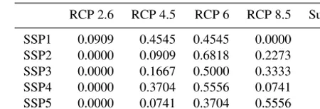
Table 3.Conditional probabilities (ranging from very low to very high) of SSPs resulting in RCPs based on authors’ judgement.
RCP 2.6 RCP 4.5 RCP 6 RCP 8.5
SSP1 very low medium medium 0
SSP2 0 very low high low
SSP3 0 low high medium
SSP4 0 medium high very low
SSP5 0 very low medium high
likelihood of SSP–RCP combinations was estimated (in the absence of mitigation strategies) as described below.
2.4.2 Assessment of the SSP–RCP scenario matrix
The SSP–RCP probability judgements were combined with the interpretation of the SSP storylines (O’Neill et al., 2016) to estimate the conditional probabilities (van Vuuren and Carter, 2014) given in Table 3. The sustainability assump-tions in the SSP1 scenario with respect to environmental and energy policies could curb emissions sufficiently to achieve RCP2.6, but it is more plausible for the SSP1 scenario to arrive at greenhouse gas concentrations consistent with RCP4.5 and RCP6.0 (medium probability).
Many medium reference scenarios result in forcing levels around 6–7 W m−2 based on a continued reliance on fossil fuels and medium population and economic growth (Clarke et al., 2014). We interpreted this as a high likelihood of forc-ing levels similar to RCP6.0 beforc-ing achieved by SSP2, SSP3 and SSP4. High-energy intensity in low-income countries and material-intensive consumption make RCP8.5 plausible in an SSP2 world, although this is assumed to have a low probability of occurrence. Given the relatively low economic growth in SSP3, we assume that forcing levels would lead to RCP6.0 or RCP8.5, with a lower probability for RCP8.5 (Table 3).
The very high-emissions pathway of RCP8.5 can only be achieved with a combination of, for example, high economic growth and reliance on fossil fuels. The divergent develop-ment in SSP4 for the few elite and the many fewer privi-leged people is difficult to estimate. We assumed that SSP4 has a high probability of resulting in forcing around RCP6.0 or possibly lower. The latter is based on the moderate pop-ulation growth and the original positioning of the scenario (small mitigation challenge). The majority of the population in SSP4 cannot afford a material-intensive lifestyle, mak-ing RCP8.5 forcmak-ing unlikely. For SSP5 we assumed that the material-intensive lifestyle combined with very high eco-nomic growth would lead to RCP8.5 with a high probability (comparable to the assumptions for the SRES (Special Re-port on Emissions Scenarios) A1F1 scenario; see van Vuuren and Carter, 2014).
The qualitative probabilities in Table 3 were translated into quantitative values in Table 4. We assumed that the
qualita-Table 4.Scenario matrix translated to quantitative probabilities.
RCP 2.6 RCP 4.5 RCP 6 RCP 8.5 Sum
SSP1 0.0909 0.4545 0.4545 0.0000 1
SSP2 0.0000 0.0909 0.6818 0.2273 1
SSP3 0.0000 0.1667 0.5000 0.3333 1
SSP4 0.0000 0.3704 0.5556 0.0741 1
SSP5 0.0000 0.0741 0.3704 0.5556 1
tive notions of very high, high, medium, low, and very low probability translated into quantitative probabilities of 0.9, 0.75, 0.5, 0.25 and 0.1 respectively. The assigned probabili-ties were normalized so that the sum of probabiliprobabili-ties for each SSP equalled 1 (see Table 4).
2.4.3 Sampling the climate-driven parameters: yields
The probabilities of SSPs resulting in RCPs (Table 4) were combined with the uncertainties arising from the climate variability of the different GCMs. To do so, the aggregated country-level yield time series (described in Sect. 2.2) were calculated for each RCP–GCM combination. Yield time se-ries calculated for different countse-ries vary, depending on the underlying GCM. To account for this spatial variability, the deviations from the yields averaged per RCP (Yˆ) were de-composed using singular value decomposition (SVD, Eq. 1), whereY is the yield projections for each GCM–RCP com-bination,Yˆ is the mean over the GCM projections for each RCP, andU,SandV are factors that can be used to recon-structY− ˆY.
U, S, V=SV D
Y− ˆY
(1)
This allows sampling of per country yield projections while preserving the patterns in spatial variability resulting from the GCM–RCP yield projections. From this we constructed four sets (one for each RCP) of 51 future yield projections, where 50 are random samples calculated using (Eq. 2) where V is replaced with ε N(0,1) and one set with the mean yield across the GCMs (ε=0). 51 samples were chosen to allow enough variability in the effect of the GCMs on the yield projections.
Y= ˆY+U Sε, ε N(0,1) (2)
2.5 Analysis of uncertainty results and sensitivity assessment
Cropland distributions with and without climate variability were analysed for the 7200 and 3600 runs respectively to the year 2100 with respect to convergence and or divergence across the five scenarios. We report the mean development and ranges at 95 % confidence levels (corresponding to 2 standard deviations) for the global-scale, model outputs, i.e. population, GDP, cereal consumption, meat consumption, feed demand, cereal demand, cereal production, cereal yield and cropland. The word “likely”, based on the IPCC’s rec-ommendation for uncertainty communication (Mastrandrea et al., 2010), was used to report results that are probable at 68–100 %. A global sensitivity analysis (GSA; Saltelli et al., 2008) was carried out to quantify the contribution of the input parameters to the uncertainty of the global cropland extent for all socio-economic model input parameters. The GSA was implemented as previously described in Engström et al. (2016), withn=5000 andp=24, requiring 130 000 runs for each scenario (according to (p+2)×n=number of runs; Lilburne and Tarantola, 2009). We used the Sobol–Jansen method (Pujol et al., 2015), which is an R implementation of the Monte Carlo estimation of Sobol sensitivity indices (Jansen, 1999; Saltelli et al., 2010), as a method that is ro-bust for large and small total indices (Saltelli et al., 2010). The total indices (hereafter, total importance) consist of the first-order effect of each input parameter and their interac-tion effects. We excluded the parameters that describe the allocation of cropland changes to forested or grassland ar-eas (grassForest) and the forest degradation rate (forestDeg) for the global sensitivity analysis because they have no direct impact on global cropland. We used the GSA to visualize the total importance, which describes the main effect and inter-action effects of the uncertainty for each input parameter on the model output (cropland).
3 Results
3.1 Ranges of global cropland projections
Global cropland area increases initially for all scenarios but declines in the simulations for F1 after 2015 (Fig. 3a). F1 continues to decline to 963±140 Mha of global cropland by 2100. All other cropland futures increase until 2030; there-after, the rate of increase slows for F2, F4 and F5. Mean global cropland peaks for F5 in 2045, and shortly afterwards for F2, and then decreases to 1400±382 Mha in 2100 for F5 and 1590±332 in 2100 for F2. For F3, global cropland con-tinues to increase over the entire simulation period, reaching 2280±200 Mha in 2100. Mean global cropland changes for F4 are very moderate throughout the simulation period and are within the cropland development of the other scenarios (1540 Mha in 2100). However, the range of cropland futures for F4 for the 95 % confidence interval in 2100 is very wide
Figure 3. (a)Cropland development from 2000 to 2100 for the five cropland futures (solid line: mean; range with dashed lines:
±2 standard deviations).(b)PDFs fitted to all runs for each
sce-nario in 2100, solid lines are runs with sampling yield variations due to GCM patterns and the scenario matrix, and dashed lines are runs where the mean yield was used.
(1126–1954 Mha). The cropland distribution of F4 overlaps with the cropland distributions of all other scenarios, as do the cropland distributions of F2 and F5. F1 by contrast has the smallest cropland range, which is also indicated by its peaked distribution (Fig. 3b).
The cropland distribution for F1 is skewed toward the higher end, which is due to the truncated distribution of un-certainties in the population projections. For the same reason, the distribution of F3 is slightly skewed toward the lower end. The cropland distribution in F3 is also peaked, indicating that the confidence in the model outcomes for F1 and F3 are the highest, despite the fact that these two scenarios show diver-gent global cropland development.
Figure 4.Global population, GDP, cereal consumption, meat consumption, cereal feed, cereal demand, mean cereal yield and cereal
pro-duction for the five scenarios F1–F5. Solid lines indicate the scenario mean; dashed lines indicate the range based on the mean±2 standard
3.2 Socio-economic dynamics influencing cropland futures
The strongly overlapping cropland ranges for the F2, F4 and also F5 scenarios are caused by the assumed uncertainties in the trends of the different input parameters but also by the counteracting effect of different scenario drivers leading to similar cropland futures. Conversely, the distinct develop-ment of cropland for the F1 and F3 scenarios is mainly due to the reinforcing dynamics of drivers as described below.
In contrast to the other population scenarios, the total pop-ulation size in F3 does not peak in the 21st century but grows continuously to 12.1±1.5 billion people by 2100 (at the 95 % confidence interval, Fig. 4a). This steady increase in population influences cereal consumption, cereal demand and (less clearly) cereal production (Fig. 4c, f and h) and thus cropland (Fig. 3). The strong population growth and there-fore high food demand is counteracted by the low economic growth in F3, which results in the relatively lower consump-tion of animal products (Fig. 4d), corresponding to 53 kg of meat per person in 2100. However, in spite of this, slow tech-nological change reinforces the high demand for cereals due to the steady increase in cereal feed (Fig. 4e).
For F5, despite a decline in total population size to 7.4±0.9 billion people by 2100, the consumption of animal products by 2100 is 820±150 Mt meat and 1230±242 Mt milk. The former corresponds to an average meat consump-tion of 110 kg meat per person in 2100, which is comparable to current meat consumption rates of several developed coun-tries, e.g. the US, Australia and Austria (FAOSTAT, 2015). The consumption of animal products is driven by economic growth and a very resource-intensive lifestyle for all con-sumption groups. For scenarios with strong technological growth, i.e. F1 and F5, the efficiency of the production of meat and dairy products increases and thus the demand for total cereal feed decreases.
Likewise, strong economic growth and technological change result in high global average cereal yields in 2100 for F1 and F5, 5.4±0.5 and 5.6±1.0 t ha−1, respectively (Fig. 4g). For F5, the strong technological growth and result-ing high yields and the high consumption levels balance the need for global cropland changes. For F1, the high yields and low consumption levels reinforce the diminishing need for cropland. By contrast, for F3, the increase in yield from 3.1 to 4.1±0.7 t ha−1and the expansion of cropland from 1503 to 2280±200 Mha in the period 2000–2100 is not sufficient to keep up with rising cereal demand (including the demand from overproduction). In 2100 global cereal demand for F3 is 4550±718 Mt, but production is 3960±814 Mt. This in-adequate global production would lead to cereal shortages and in a few cases to countries approaching their maximum available arable land. More importantly, the underproduction is due to incentives for exporting countries to increase their production, as well as cropland degradation, that are insuffi-cient, though conceptually consistent with SSP3.
3.3 Uncertainty in socio-economic model inputs
The uncertainty in input parameters contributes differently to the uncertainty of global cropland futures over time (Fig. 5). For F1, population projections and technological change dominate uncertainty, the latter being especially important during the first quarter of the simulation period. Similarly, for F2, uncertainties in technological change and consump-tion are at first important, but after 2025 cropland degrada-tion contributes largely to the uncertainty of global cropland. By contrast, population projections and technological change are the major contributors to the uncertainty range of global cropland for F3. For F4, uncertainties in the extent of land degradation, but also population projections and consump-tion and technological change, contribute to uncertainties in global cropland. Consumption and technological change be-come less important over the 21st century, compared with land degradation and population. These trends are similar for F5.
4 Discussion
For F2, F4 and F5, the uncertainty distributions of global cropland overlap greatly, with cropland changes over the 21st century within the range of−20 to+17 %. This large overlap can be explained by counteracting drivers but also by larger uncertainties in the assumptions of model input parameters for the SSPs with contrasting directions of change in chal-lenges for mitigation and adaptation (i.e. SSP4 and SSP5). By contrast, the F1 and F3 cropland futures are very distinct from one another, with a higher level of confidence, indicated by their peaked distributions. The simulated discrepancy be-tween total demand and production in F3 indicates that a fo-cus on regional production with limited trade can risk food insecurity for countries with limited potential for domestic production, which agrees with Brown et al. (2014). When considering F1 and F3, the F2, F4 and F5 range of cropland changes by 2100 (−20 to+17 %) increases to a total range of−41 to 58 % by 2100 compared with 2000. These results lead to a slightly larger uncertainty range compared with deterministic scenario projections. For example, the crop-land changes simulated by four different integrated assess-ment models (IAMs) were 1130–2100 Mha cropland by 2100 (RCP4.5-GCAM and RCP2.6-IMAGE; Hurtt et al., 2011). This corresponds to cropland changes from 1990 to 2100 of−25 to +39 % (Hurtt et al., 2011). It is difficult to com-pare these results directly since the IAM scenarios also in-clude land-based mitigation options. For example, the crop-land changes in RCP2.6-IMAGE were the result of a strin-gent mitigation scenario, where the production of biomass for bioenergy increased cropland areas (Hurtt et al., 2011).
F1 F2 F3 F4 F5
Population input data (no. 0, )pop
Level of food production (no. 1)
Consumption lifestyle (nos. 2–4)
Technological change (nos. 5–6)
Land degradation (no. 12)
Figure 5.Total importance of global cropland for the futures F1–F5 to uncertainty of input parameters, aggregated to input parameter groups as in Table 2 (for non-aggregated results, see Fig. C1 in Appendix C).
bioenergy production, could be implemented on abandoned cropland without compromising food security or the provi-sion of other ecosystem services. However, the global sen-sitivity analysis showed that for F1 to consistently achieve strong decreases in cropland areas, it is important to stay within the range of input assumptions. Among others, con-sumption patterns have to reflect the more resource efficient and environmentally friendly lifestyle that underlies this sce-nario. Achieving technological change and thus yield in-crease is important, as is dein-creased environmental degrada-tion and thus decreased cropland degradadegrada-tion rates.
The LPJ-GUESS yield projections are at the higher end of the range of yield projections compared with other mod-els (Rosenzweig et al., 2013) and likely overestimate the ef-fect of CO2fertilization since nitrogen limitations were not
included in earlier versions of the model. However, these effects were counteracted in PLUM by (a) dividing global production by global cropland area to derive global aver-age yield, which does not account for double cropping, and (b) assumptions about cropland degradation that are imple-mented as a production loss, which decreases the simulated global average yield. Future research will consider the man-agement options in LPJ-GUESS coupled to PLUM (e.g. the use of irrigation and fertilization scenarios) and will improve the potential impacts of climate change on yields arising from pests and heat stress. Currently, heat stress implementa-tion in LPJ-GUESS is limited to a shortened growing season, increased respiration and lowered photosynthesis.
The sensitivity analysis showed that assumptions about cropland degradation were important for cropland devel-opment across all scenarios. Cropland degradation was as-sumed to lead to an average global production loss of be-tween 6 % (F1) and 14 % (F5) in 2100. This compares with an estimated global average of 20–40 % loss of potential pro-duction on degraded agricultural areas only (Zika and Erb, 2009). Hence, the PLUM results of total global production (not only on degraded agricultural areas) appear to be of the
right magnitude and the sensitivity analysis highlighted the importance of accounting for these uncertainties.
Global cropland was less sensitive to the uncertainties associated with the consumption input parameters, which, for example, describe the rate of increase or decrease in meat consumption for the four consumption country groups. PLUM represents cultural differences in consumption pat-terns between countries (based on four consumption groups), but this could potentially mask part of the total importance of the consumption input parameters because the correla-tion between the parameters of the four consumpcorrela-tion groups was not considered. Additionally, cropland changes are likely to be underestimated in F5 because meat consumption in-creases strongly in countries currently defined as developing and global average meat consumption approaches 110 kg per person in 2100. This would probably be associated with the intensification of animal production, which currently is not included in PLUM. Since intensive meat production would lead to an increase in the feed share derived from cereals, cropland areas would increase.
transparency in the assumed parameter ranges and distribu-tions. Overall, the conditional probabilistic approach applied in PLUM led to cropland area ranges that are consistent with those reported by other scenarios and model intercomparison studies (Alexander et al., 2016; Hurtt et al., 2011; Prestele et al., 2016; Schmitz et al., 2014), which provides confidence in the modelling framework. PLUM is based on cereal demand and assumes that changes in cereal land are a reliable proxy for food demand and cropland changes with free-trade con-tributing greatly to meeting demands. For example, a change in the demand of cereals compared to other crops driven by climate change (either directly, or by enhanced demand for bioenergy) will require a revision to the constant cereal– cropland ratio. Future model development will take bioen-ergy production into consideration. The global-scale projec-tions with PLUM need to be interpreted under the assump-tion that the future agricultural system will not be fundamen-tally different from how we understand it today; an assump-tion that occurs in most global models. Clearly, in some sce-narios the free-trade simplification might not be valid (e.g. in SSP3), a limitation that is balanced by PLUM having simple and transparent relationships. We argue that the possibility to perform rapid model runs outweigh drawbacks in the cur-rent model version that arise from less than perfect regional model performance.
High-end climate change impacts on yields (i.e. from solely applying RCP8.5) were not tested here, as the goal of this study was to create plausible and consistent crop-land futures that address the uncertainties within each sce-nario rather than assessing the impact of each emission path-way. Excluding high-end climate change impacts on yields explains why the variability in climate change was found to have a relatively small impact on global cropland areas. Small differences in the climate change impacts on agricul-tural areas between RCP4.5 and RCP6.0 were found else-where (Wiebe et al., 2015), as well as the comparatively larger effects of RCP8.5. The approach used here, based on a matrix populated with probabilities, streamlined the total number of scenarios and simultaneously removed the need to compromise with single selections of SSP–RCP combina-tions.
5 Conclusion
Considering the simple supply and demand mechanism in the model (the use of cereals as a proxy for demand and area changes), the likely range of global cropland simulated in this study ranged from 893 to 2380 Mha in 2100. This was consistent with the range reported in the literature of 930–
2670 Mha in 2100, although slightly skewed to the lower end of this range. This shows that uncertainties in input as-sumptions are equally important for output ranges as differ-ences in the model structure and that the entire uncertainty of global cropland development is probably even larger if these sources of uncertainties are combined. Considering the certainties in input assumptions, we found that the deep un-certainties reflected in assumptions for the socio-economic scenarios contributed most to the total magnitude of the pro-jected cropland range. The uncertainties in scenario interpre-tation widened the total projected future cropland range and led to overlap in the simulated cropland areas for three out of five scenarios. Cropland futures where the output PDFs did not overlap with other scenarios were found for the SSP1 sce-nario projections and the SSP3 scesce-narios, whereas the SSP2, SSP4 and SSP5 scenarios were found to have large areas of overlap. This was partly due to the compensating dynamics of drivers, e.g. strong yield development and increase in con-sumption in the SSP5 scenario, but also due to the larger un-certainties in scenarios with contrasting challenges for miti-gation and adaptation (i.e. SSP5 and SSP4 scenarios). Uncer-tainties in population projections, technological change and cropland degradation were found to be the most important for uncertainty in global cropland projections, while uncertain-ties in consumption levels and production levels were found to be less important. When taking account of the uncertainty ranges at the 95 % confidence interval across all scenarios, there were fewer differences between the scenarios, i.e. there is overlap at some level of probability in all global cropland projections, except for projections based on SSP3. This leads us to conclude that very different worlds can result in very similar cropland futures on the aggregated global scale as long as they share low to medium population development.
6 Data availability
Appendix A: Model development
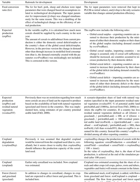
A1 Changes compared to previous PLUM version
In comparison to the version described in Engström et al. (2016), several minor alterations (Table A1) and one larger alteration were made to the model. The larger alteration relates to the representation of the yield development in PLUM, which is explained below. Assumptions are also made within PLUM about the scenario dependency of the availability of potential arable land (residualNV), reflecting different environmental policies in the SSPs.
A2 Yield development in PLUM
The global parameter6_technologydescribes the change in trend of technological development. The parameter 6_invest-mentcharacterizes how much yield increases as a function of GDP per capita. The parameter6_distributiondescribes how agricultural management practices are assumed to be trans-ferred across and within countries. For example, in a scenario with an emphasis on human development, it is assumed that the distribution of technologies would be more efficient and thus the yield gap would decrease more rapidly, compared to a scenario that only emphasizes investment in technology but not its distribution. Here we assumed that6_distribution
is negatively correlated to the percentage of rural population (derived from the urban share projections from 2010 to 2100 NCAR, v9_130115; SSP Database, 2015) on the basis that a larger share of rural population implies more small-scale farming with simple technologies and lower yields. Addi-tionally, the variables in Table A2 were added during the implementation of LPJ-GUESS-driven yield development in PLUM.
Cereal yield cerealYieldC is calculated in the following way:
cerealYieldC=if cerealYield×shareYieldi>
cerealYieldFAOi×boundarySharethen cerealYield×
shareYieldielse cerealYieldFAOi×boundaryShare.
To avoid yields decreasing to 50 % (corresponding to default
boundaryShareof 0.5) or less than the initial (i) FAO value (cerealYieldFAOi) cerealYieldC is kept constant in this case.
The LPJ-GUESS-based calculated yield (cerealYield) is nor-malized with FAOSTAT cereal yield by multiplying with shareYieldi.
shareYieldi=cerealYieldFAOi/yieldAi
cerealYieldtis calculated as follows:
cerealYieldt=yieldPt×(1−yieldGapt).
yieldGapt is calculated as follows:
yieldGapt =1− yieldAt×kt/(yieldPt)
.
The functionkt determines how much of actual yield vs. po-tential yield is produced during time:
If q <0.98, then
kt=kmaxt×(1−(ht×qt)) elsekt =kmaxt(1−(ht×0.98).
The maximum value of kmaxt is
kmaxt=yieldPt/yieldAt.
The functionht:
ht=(1−(1/kmaxt))/qi.
The functionqt describes the impact of investments in tech-nology and distribution of techtech-nology on yields. Investments in technology are here assumed to be dependent on income growth (GDP per capita), and distribution of technology is assumed to be related to the share of urban population in to-tal population.
qt=exp −technolt−investmentt×gdpPct + distributiont×(100−urbanSharet))
The functions technolt, distributiont and investmentt allow the change in the initial factors which were found by regres-sion analysis based on statistical analysis of data for the year 1995–2005:
technolt=0.77+6_technology/100×time()
investmentt =(1.80+6_investment/100×time())×10−5 distributiont =(2.55−6_distribution/100×time())×10−3. The scenario-dependent input parameters 6_technology,
Table A1.PLUM development, affected variable, rationale for development and implemented development.
Variable Rationale for development Development Food conversion
ratio (fcr)
The fcr for beef, pork, sheep and chicken were input parameters that were changed based on assumptions re-lated to technological development. The input param-eter fcr improvement (fcrImp) was changed simultane-ously for the same reason. This was a doubling of the effect of technological change on the efficiency of ani-mal production.
The fcr input parameters were removed (but kept in PLUM as initial values), andfcrImpis the only scenario variable that changes animal production efficiency.
Expected production (expPro)
In the variable expPro, it is calculated how much more cereals should be supplied by each country in the next year.
The amount of cereals to add/subtract from current pro-duction is either the domestic cereal deficit/surplus or the country’s share of the global cereal deficit/surplus. However, in the previous version the change in demand other than through increase in modelled food consump-tion (that is, the demand externally created with the pa-rameteroverProdRate) was misleadingly not included. This is corrected in this version.
The expPro now includes the following rules:
– Global cereal surplus – exporting countries are as-sumed to decrease their production by the mini-mum of either their domestic surplus or their share of the global surplus (including demand created byoverProdRate).
– Global cereal surplus, importing countries – no change is assumed; only if cereal self-sufficiency should be increased, are countries assumed to in-crease production by their domestic deficit.
– Global cereal deficit – exporting countries are as-sumed to increase their production by their share of the global deficit (including demand created by
overProdRate).
– Global cereal deficit – importing countries are as-sumed to increase their production by the maxi-mum of either their domestic deficit or the share of the global deficit (including demand created by
overProdRate).
Expected production (expPro) and residual natural vegetation (residualNV)
Previously there was no restriction regarding how much more cereals an area of land can be expected to produce based on the availability of land with natural vegetation (grassland and forest) in the countries. This was imple-mented here, using estimates of per country potential arable land (FAO, 2000).
A scenario-dependent share of land with natural veg-etation (specified in the input parameter residual natu-ral vegetation (residualNV; % of potential arable land potArableLand (1000 ha, derived from FAO, 2000)) re-stricts the expPro for countries. If a country has less residual natural vegetation (defined as all ((forest +
grassland)/ potArableLand) ×100, or if ((forest +
grassland)/ potArableLand)× 100 < residual poten-tial arable land (resPotAL=((potArableLand− cere-alland−restCropland)/potArableLand)×100), then resPotAL) left thanresiudalNV), then no expPro is as-sumed for this country. Instead this country’s expPro is divided among all other exporting countries.
Cropland degradation (croplandDeg)
Previously it was assumed that degraded cropland would be removed from the cropland used (that is, cere-alland), but it seems closer to reality thatcroplandDeg
should influence the production capacity of the cereal-land used.
croplandDegchanges the production of cereals with the following equation: cerealProduction= cerealland×
cerealYield−cerealland×cerealYield×croplandDeg /100×time().
So the value ofcroplandDeg, that is, the share of lost production, is achieved at the end of the simulation pe-riod (after 100 years).
Cropland (cropland)
Earlier only cerealland was included. Now cropland was estimated.
Cropland was estimated assuming that the share of ce-reals and other crops (oil crops, pulses, roots and tubers, vegetables and fruits) will remain constant in the future. Forest (forest)
and grassland (grassland)
In addition to changes in cerealland, changes in crop-land are expected to affect forest and grasscrop-land. This is included here.
One additional stock, restCropland, is added, with flows from grassland and forest. restCropland is cropland−
Table A2.Yield-related variables in PLUM.
Variable type Variable name Source
Initial value cerealYieldFAOi FAOSTAT, 2015
Initial value yieldAi First year of yieldA_t (currently year 2000)
Initial value qi q_t at time 0, i.e. year 2000 in this version
Time series yieldPt LPJ-GUESS, potential yield
Time series yieldAt LPJ-GUESS, actual yield
Time series gdpPct Income growth, GDP per capita, SSP data
Time series urbanSharet Share of population living in urban areas, SSP data
Model parameter boundaryShare Share of cerealYieldFAOithat yield can decrease
Appendix B: Input to the conditional probabilistic approach
B1 Extended SSP narratives
B1.1 SSP1: sustainability – taking the green road
Key themes: Cooperative countries, environmentally
friendly, functioning markets
Facilitating governance and institutional structures, coop-erative countries, environmentally conscious societies and decreased inequalities contribute in this SSP to the progress towards a sustainable world, including lower population growth. Due to effective international institutions and good information flow between markets, governments and farm-ers and functioning global markets, agricultural areas are de-creased rapidly in case of food overproduction. Countries rely on regional trade, and attempts are made to keep food stocks low in order to be resource efficient. The conver-sion of natural land to new cropland is well regulated in most countries to avoid substantial deforestation and biodi-versity loss. Investments in agriculture and agricultural re-search stay high in high-income countries, and local, context-dependent agricultural best-management practices (includ-ing non-conventional practices, e.g., no tillage) are imple-mented in most countries. The investment in technology con-tinues to result in more efficient animal protein production. An additional important factor for globally increasing yields is the technology transfer between countries and income lev-els. Equity and education are important in this scenario and contribute to yield improvements as well. The awareness for resource efficiency also decreases food waste and the con-sumption of refined products, which leads to a decreasing cereal consumption. The environmental awareness of con-sumers leads to a slowing down and an eventual decrease in the consumption of dairy and meat products. However, low-income countries moderately increase their animal prod-uct consumption until they reach consumption levels that are common among western countries. Environmental degrada-tion slows down and the status of land improves, thanks to increasing implementation of holistic and sustainable man-agement and afforestation programs.
B1.2 SSP2: middle of the road
Key themes:Business as usual
In SSP2 trends observed during recent decades con-tinue, including some reductions in resource intensity, but mostly large inequalities between countries and economies remain. Technological development is moderate and preinary, concentrated in high-income countries. Due to lim-ited technology transfer, low-income countries do not benefit from advances in agricultural management and yields remain rather low. Agricultural markets are partially functioning and globally connected, but trade barriers are only reduced slowly. Some countries with limited access to global markets
focus more strongly on increased domestic production and self-sufficiency. In general food stocks are held at moderate levels and the abandonment of cereal land remains unregu-lated. For new cropland generation, high-income countries follow existing regulations, while in some low-income coun-tries with rich natural resources unregulated deforestation for cropland generation continuous to be a problem. Environ-mental degradation continues at historical rates, as no serious efforts are made to achieve large-scale sustainable land man-agement. Additionally the continuing increasing demand for animal products contributes to expansion and intensification of agriculture with some negative environmental impacts.
B1.3 SSP3: regional rivalry – a rocky road
Key themes:World regions, security of regions, no progress
in technologies
In the fragmented world, regional blocks form, with lit-tle international cooperation and protectionist policies of re-gions as a result. This leads to little reduction of land in-tensity, low technological development and generally slow economic growth but high population growth. However, in some areas wealth moderately increases, and so does tech-nological development. The increasing efforts of regions to be more food self-sufficient reduce agricultural trade and in-crease the food overproduction within regions to ensure suf-ficient food supply in case of regional harvest shortcomings. Consequently, agricultural area is only abandoned at a very slow pace, even if a region is food sufficient. At the same time, weak governance and institutional structures do not provide any strong regulations reducing the conversion of natural land to cropland. Forests and natural grasslands are converted into cropland at faster rates to ensure regional food security. Food consumption, and in particular the consump-tion of animal products, continues to increase in most regions but at a slower pace for low-income countries. The increased demand for food and the non-regulated land use change re-sult in serious environmental degradation.
B1.4 SSP4: inequality – a road divided
Key themes:The few wealthy control, the rest struggles
rates to new cropland without considering environmental and social effects. The absence of sustainability regulations leads to serious environmental degradation, affecting the poor and making them even more vulnerable. The global food trade is dominated by the industrial agricultural businesses with very limited access for small-scale farmers. Small-scale farmers therefore rely more on self-sufficient agricultural systems. While the privileged society increases its consumption of an-imal products, the large group of poor people cannot afford large increases in meat and dairy consumption. The overall demand for food production does therefore not proportion-ally increase with the high population growth, as most of the world’s people cannot afford an expensive diet in times of economic uncertainty.
B1.5 SSP5: fossil-fuelled development – taking the highway
Keywords: Resource intensive, no compromises to gain
ma-terial wealth
In this world economic, resource-intensive development is prioritized, and while this leads to eradication of extreme poverty, it comes at environmental costs. Developing coun-tries are pushed in their development, and soon all councoun-tries share a resource-intensive lifestyle, including high levels of animal product consumption. The high demand for these and other agricultural products is fulfilled by highly engineered agricultural systems. Investment into agricultural technology is very high. Increasing agricultural specialization of coun-tries is common too; however, it is often connected to very resource-intensive production, both in terms of water and fertilizers. Agricultural area also expands into natural areas at faster rates if necessary. Solutions to environmental prob-lems do not tackle the problem’s roots, but only its symp-toms. However, the global food market functions well and keeps the total food stock decrease slow.
B2 Examples of rationales for changes in trend and uncertainty levels for PLUM input parameters conditional on SSPs
An example of the importance of being explicit about base-line trends is the following: in SSP5 the very strong trend of technology improving agricultural management (Table 1; SSP5;technology:+ + +) is, when compared to the gener-ally strong baseline trend of technology (++), not consid-ered extreme. To illustrate this approach further, consider for instance the scenario element “globalization” from Ta-ble 2, which we assumed will influence, jointly with sce-nario elements “international trade” and “agriculture”, the input parameter that guides the level of food production in the model. If we take SSP3, a degree of de-globalization and enhanced regional security is assumed to be taking place in future (O’Neill et al., 2016). Consistent with a world where the trend of globalization is reversed and regional security
is important, we assumed for SSP3 that production levels would be higher (+ + +, Table 1) compared to the current trend in order to ensure the satisfaction of demand internally. The opposite is true for SSP1, where “globalization” leads to “connected markets, regional production” (O’Neill et al., 2016). We assumed that production levels would be lower (−−; Table 1) than present-day levels since food would be distributed more efficiently around the globe. The reduction of production levels would also decrease food waste, which is consistent with SSP1’s “policy orientation” towards sus-tainable development.
B3 Quantitative values for input parameters
For each scenario and each input parameter, quantitative val-ues were derived by sampling from Table B1 based on the scenario and input parameter’s qualitative notions in Table 1. This matrix (Table B1) was populated by first placing the (baseline) mean value (Engström et al., 2016) based on the quantitatively estimated baseline trend within the ma-trix. Secondly, we identified minimum and maximum values for each input parameter, based on statistical analysis of his-toric data or the authors’ judgement as described in Engström et al. (2016). Thirdly, these values informed the extremes (−−−and+++), and the entries between the extremes and the baseline mean values were filled with evenly interpolated values. The quantitative values for the qualitative uncertainty levels low, medium and high were informed by variability in historic data. We assumed the historic standard deviations to be generally high because data were analysed over a time pe-riod (1961–1990) where substantial changes in consumption and production patterns led to high heterogeneity in the data (Alexander et al., 2015). We used the historic standard devia-tion for the high uncertainty value. The medium and the low uncertainty values are two thirds and one thirds of the high uncertainty level respectively (Table B1).
Table B1.Matrix with quantitative values for changes in trend from− − −to+ + +(mean values) and the uncertainty levels low, medium
and high (1 standard deviation, SD). Values are based on analysis of historical data, except that values withawere estimated by the author
(see Engström et al., 2016). Superscript b indicates that values are maximum values rather than standard deviations. Values in bold are baseline values, corresponding to the baseline trend in Table 1.
No. Input parameter (unit) Change in trend, mean values Uncertainty, 1 SD
− − − −− − 0 + ++ + + + Low Medium High
0 gdpVar(%) country-level time series for each SSP calculated based on other
0 popVar(%) projections; see Table 1
1 overProdRate(1/time) −0.004 −0.003 −0.002 −0.001 0.000 0.001 0.002 0.0002 0.0004 0.0006 2 cerealVar(1/time) −0.003 −0.002 −0.001 0.000 0.001 0.002 0.003 0.0002 0.0004 0.0006 3 meat 1(kg meat per capita/log(GDP per capita)) −10.0 −5.0 0.0 5.0 10.0 15.0 20.0 2.0 4.0 6.0 3 meat 2(kg meat per capita/log(GDP per capita)) −6.0 −3.0 1.0 3.0 5.0 10.0 15.0 1.0 2.0 3.0 3 meat 3(kg meat per capita/log(GDP per capita)) −5.0 0.0 5.0 10.0 15.0 20.0 25.0 1.0 2.0 3.0 3 meat 4(kg meat per capita/log(GDP per capita)) −2.5 0.0 2.5 5.0 10.0 15.0 20.0 1.0 2.0 3.0 4 milk 1(kg milk per capita/log(GDP per capita)) −10.0 −5.0 0.0 5.0 10.0 15.0 20.0 2.0 4.0 6.0 4 milk 2(kg milk per capita/log(GDP per capita)) −4.0 −2.0 0.0 2.0 6.0 10.0 14.0 1.0 2.0 3.0 4 milk 3(kg milk per capita/log(GDP per capita)) −5.0 0.0 5.0 10.0 15.0 20.0 25.0 2.0 4.0 6.0 4 milk 4(kg milk per capita/log(GDP per capita)) −2.5 0.0 2.5 5.0 10.0 15.0 20.0 2.0 4.0 6.0 5 fcrImpa(1/time) −0.002 −0.001 0.000 0.001 0.002 0.003 0.004 0.0003 0.0006 0.0009 6 distribution(1/time) −1.00 −0.66 −0.33 0.00 0.33 0.66 1.00 0.15 0.30 0.45 6 technology(1/time) −0.125 −0.080 −0.040 0.000 0.040 0.080 0.125 0.030 0.060 0.090 6 investment(1/GDP per capita×time) −0.65 −0.43 −0.21 0.00 0.21 0.43 0.65 0.10 0.20 0.30 7 abandonCLb(unitless) 0.010 0.015 0.020 0.023 0.040 0.055 0.070 0.003 0.006 0.009 7 abandonCL_Db(unitless) 0.010 0.011 0.013 0.015 0.025 0.035 0.050 0.003 0.006 0.009 8 newCLb(unitless) 0.010 0.011 0.013 0.015 0.250 0.035 0.048 0.003 0.006 0.009 8 newCL_Db(unitless) 0.010 0.018 0.025 0.029 0.035 0.040 0.045 0.003 0.006 0.009 9 newCLsb(unitless) 0.000 0.000 0.000 0.000 0.015 0.030 0.048 0.003 0.006 0.009 9 newCLs_Db(unitless) 0.010 0.018 0.025 0.029 0.035 0.040 0.045 0.003 0.006 0.009
10 grassForesta(unitless) 0.50 0.50 0.50 0.50 0.50 0.50 0.50 0.03 0.06 0.09
11 residualNVa(%) 4.0 6.0 8.0 10.0 12.0 14.0 16.0 1.0 2.0 3.0
12 croplandDega(1/time) 0.04 0.06 0.08 0.10 0.12 0.14 0.16 0.03 0.06 0.09
Appendix C: Additional output
F1 F2 F3 F4 F5