https://doi.org/10.5194/amt-11-2119-2018 © Author(s) 2018. This work is distributed under the Creative Commons Attribution 4.0 License.
Estimation of nocturnal CO
2
and N
2
O soil emissions from
changes in surface boundary layer mass storage
Richard H. Grant and Rex A. Omonode
Department of Agronomy, Purdue University, West Lafayette, Indiana, 47907, USA
Correspondence:Richard H. Grant ([email protected]) Received: 28 July 2017 – Discussion started: 31 August 2017
Revised: 30 January 2018 – Accepted: 18 February 2018 – Published: 12 April 2018
Abstract. Annual budgets of greenhouse and other trace gases require knowledge of the emissions throughout the year. Unfortunately, emissions into the surface boundary layer during stable, calm nocturnal periods are not measur-able using most micrometeorological methods due to non-stationarity and uncoupled flow. However, during nocturnal periods with very light winds, carbon dioxide (CO2) and ni-trous oxide (N2O) frequently accumulate near the surface and this mass accumulation can be used to determine emis-sions. Gas concentrations were measured at four heights (one within and three above canopy) and turbulence was mea-sured at three heights above a mature 2.5 m maize canopy from 23 July to 10 September 2015. Nocturnal CO2 and N2O fluxes from the canopy were determined using the ac-cumulation of mass within a 6.3 m control volume and out the top of the control volume within the nocturnal surface boundary layer. Diffusive fluxes were estimated by flux gra-dient method. The total accumulative and diffusive fluxes during near-calm nights (friction velocities < 0.05 ms−1) av-eraged 1.16 µmol m−2s−1CO2and 0.53 nmol m−2s−1N2O. Fluxes were also measured using chambers. Daily mean CO2 fluxes determined by the accumulation method were 90 to 130 % of those determined using soil chambers. Daily mean N2O fluxes determined by the accumulation method were 60 to 80 % of that determined using soil chambers. The bet-ter signal-to-noise ratios of the chamber method for CO2 over N2O, non-stationary flow, assumed Schmidt numbers, and anemometer tilt were likely contributing reasons for the differences in chambers versus accumulated nocturnal mass flux estimates. Near-surface N2O accumulative flux mea-surements in more homogeneous regions and with greater depth are needed to confirm the conclusion that mass
accu-mulation can be effectively used to estimate soil emissions during nearly calm nights.
1 Introduction
shal-low surface boundary layer that thickens over time through light continuous or intermittent turbulence into a stable noc-turnal boundary layer on the order of 100 m deep (Kaimal and Finnigan, 1994). Xia et al. (2011) noted an accumulation of 222Rn within a 6.5 m deep surface boundary layer over a grass clearing of a forest preserve during nights with clear sky, light winds, and strong radiative cooling. Similar gas ac-cumulations in the surface boundary layer at night have been conducted for CO2, CH4, and N2O over pastures and crops (Pattey et al., 2002; Pendall et al., 2010). As weak turbulence mixes the surface boundary layer air with the cooling stable nocturnal boundary layer, gas mass accumulations become evident throughout much of the stable nocturnal boundary layer. Such mass accumulations are reported for CO2, CH4, and N2O over crops, plantations, and forests (Pattey et al., 2002; Acevedo et al., 2004, 2008).
Using temporal mass accumulation for estimating flux un-der stable conditions assumes that horizontal mass transport is negligible, there are no local sources of N2O or CO2within the control volume, and the exchange of mass between the control volume and the overlying air is minimal. If there is no flow in the surface boundary layer (SBL), then gases emit-ted from the soil surface will diffuse upward at roughly the rate of molecular diffusion (approx. 10−5m2s−1). Such con-ditions are approximated in soil flux chambers but do not oc-cur in the surface boundary layer beyond the laminar layer at the surface. Compared to the typical turbulent diffusion exchange coefficients, the molecular diffusion rate is neg-ligible. Consequently gas diffusion from the surface is ef-fectively stopped at any altitude when the diffusion rate de-creases a few orders of magnitude. This provides the effective “cap” on the mixing of gases in the control volume layer.
Many approaches have been used to define the conditions in which the accumulation of a gas as effectively capped in the surface boundary layer. Since the friction velocity (u∗)
provides an index of turbulent mixing, Pattey et al. (2002) used au∗threshold for validating the quality of the cap.
Pen-dall et al. (2010) defined the top of the accumulation con-trol volume based on significant correlations between CO2 (presumed from soil respiration) and CO, CH4, N2O, and H2. The top of the control volume has been estimated by Acevedo et al. (2004) using the top of an observed fog layer or the height of constant potential temperature and specific moisture in the early morning. Acevedo et al. (2008) used the height of the strongest potential temperature inversion as the control volume top. Pattey et al. (2002) determined the accumulation over the entire 10 m of profile measurements under constrained turbulent flow conditions. Using these cap definitions, the temporal change in mass accumulations have been determined over relatively thin layers of air over crops (10 m thick; Pattey et al., 2002), pastures (5 m thick; Pendall et al., 2010), and plantations (8 m thick; Pendall et al., 2010). Other much thicker layers of at least 20 m have been defined over forests (Acevedo et al., 2004, 2008; Pendall et al., 2010).
Biraud et al. (2002) assumed stationary flow conditions at all times and found that wind speeds (at 10 m) ranging from 1.5 to 8 ms−1over 4 days corresponded to footprints extending 150 to 200 km from the measurement location.
We evaluated the nocturnal flux of CO2 and N2O from maize-cropped land based on the temporal accumulation of mass storage within the surface boundary layer constrained vertically by the flow characteristics at the top of a layer 6.3 m deep.
2 Methods
N2O and CO2 fluxes were measured using three methods during the night between 20:00 and 04:00 local time (LT) over nitrogen-fertilized fields during the summer of 2015. These fields are located in a relatively flat and homogeneous terrain (Fig. 1a) near West Lafayette, Indiana, USA (40.495◦
latitude and −86.994◦ longitude). The terrain rises to the north at a rate of only 2 m km−1 and land use is predomi-nantly agricultural, with cropped land covering 100 % of the land within 1 km2and 97 % of the within 10 km2(Table 1) and 83 % within 25 km2. Crops generally alternate between maize and soybean with 83 %, (1 km2)46 % (10 km2), and 40 % (25 km2)in maize in 2015.
The instrumented towers (described below) were situated in a tilled field (“200Sp”; Fig. 1b) in which 220 kg N ha−1 was applied as anhydrous ammonia (AA) at pre-plant in spring 2015. Three other fertilizer treatments were applied in fields near the towers: a 220 kg N ha−1AA application on a no-till field (“200Fa”; Fig. 1b), a 110 kg N ha−1AA appli-cation during the fall of 2014, followed by a pre-plant spring AA application of 110 kg N ha−1(“100Fa/100Sp”; Fig. 1b) on a tilled (north) and no-till (south) field.
N2O and CO2 concentrations were measured from air sampled out of a 7 L min−1 air flow drawn from 1 µm fil-tered inlets at three heights: 2.8, 5, and 8 m above ground level (a.g.l.). Air was sampled sequentially for 5 min at each inlet. Mean concentrations were based on the last three of each 5 min interval to account for the time lag associated with the air flow and the measuring instruments. The 2.8 m point sample was made from a mast that was 18 m from the 5 and 8 m measurement mast (Fig. 1b). In addition a line sample based on a 50 m line with 10 inlets drew air at 1 m within the canopy (Grant and Boehm, 2015). The 1 m in-canopy line sample measurement was positioned between 50 and 25 m (line sample end to end) from the 5 and 8 m single point mast measurements (Fig. 1b). The 2.8 m single point measure-ment was made between 45 and 65 m from the 1 m line sam-ple (end to end) and 18 m from the 5 and 8 m measurement mast (Fig. 1b). The N2O in the sampled air was measured using an IRIS 4600 difference frequency generation (DFG) laser mid-infrared (IR) analyzer (ThermoFischer Scientific, Franklin, MA) with a measured N2O minimum detection limit (MDL; 3σ) of 0.3 nmol mol−1. The CO2 in the
sam-pled air was measured using a LiCOR 840 non-dispersive IR analyzer (LiCOR, Inc., Lincoln, NE) with a measured CO2 MDL of 5 µmol mol−1. The moisture content of the sampled air was also determined by the LiCOR 840 non-dispersive IR analyzer. All concentrations were corrected to dry air.
Atmospheric pressure, temperature, and relative humidity were measured at 2.5 m at 5 min intervals on a weather sta-tion within 100 m of the gas measurements. Turbulence was measured at three heights (2.5, 5, and 8 m) using a three-dimensional sonic anemometer (RM Young 81000, RM Young, Inc., Traverse City, MI). Turbulence was sampled at 16 Hz and recorded at 10 Hz. The MDL was approximately 0.01 ms−1. Since the tethered towers was tilted but shifted slightly in tilt due to shifts in the wind direction, a double rotation rather than planar rotation was made to correct the flow coordinate system for each 30 min turbulence-averaging interval (Lee et al., 2004). The MDL for the friction veloc-ity (u∗)based on error propagation of the anemometer MDL
through the definition ofu∗, was estimated to be 0.014 ms−1.
In reality, the non-stationary flow conditions in the stable nocturnal boundary layer results in sensitivity ofu∗ on the
specific averaging period and consequently is more uncertain than the calculated MDL. Stability was assessed using the lo-cal Obukhov length (3)based on local measures of heat and momentum transfer within the stable boundary layer (van de Wiel et al., 2008).
The accumulation of constituent C (Qaccum,C) over the maize canopy was based on gas concentration measurements (using the DFG and NDIR instruments) made at three heights (2.8, 5, and 8 m; Fig. 1b) on an 8m tower and one height representing an integrated line concentration in the maize canopy (1 m; Fig. 1b). Accumulation flux was determined into the layer according to
Qaccum,C=
1R6.3
0 Cdz
1t , (1)
using Newtonian integration and assuming the concentration ofC (CO2and N2O) between the ground and 1 m was con-stant and equal to that at 1 m. The mass accumulative flux was calculated as the linear slope of the time-resolved accu-mulation of three measurements over 90 min. Turbulent con-ditions were segregated into those withu∗less than or greater
than or equal to 0.05 ms−1(approximately 4 times the esti-mated sensor MDL of 0.014 ms−1). This threshold was lower than that used by Pattey et al. (2002), who used a threshold of 0.1 ms−1for bothu
∗and standard deviation ofw(σw)to estimate flux by mass accumulation, and lower than that used by Wagner-Riddle et al. (2007), who used au∗threshold of
0.1 ms−1 and a Monin–Obukhov stability of less than 2 to estimate flux by flux gradient during stable boundary condi-tions.
Figure 1.Experimental domain: GoogleEarth®images from August 2015 showing the homogeneous agricultural land use across the region surrounding the experimental field (Montmorenci, Indiana, USA; 40.495◦latitude and−86.994◦longitude: panela) and the configuration of measurements in the experimental field (panelb). Fertilizer treatments (kgN Ha−1season−1) in the north field and south field (200Sp, 200Fa, 100Sp/100Fa, and no N) as well as the locations and heights of the sonic anemometers and inlets (open triangles), integrated line sample (open diamond and orange line), and meteorological station (open circle) are indicated in panel(b). Note scale in lower right corner of panel(b).
Table 1.2015 land use around the research site and literature-reported CO2and N2O fluxes for each land use.
Land use 1 km2 10 km2 CO2respiration Source N2O emissions Source
area (%)∗ area (%)∗ (µmol m−2s−1) (nmol N2O m−2s−1)
Maize 83 47 Soil/root: 0.9–1.8 Omonode et al. (2007) 0–2.1 Eichner (1990)
production Canopy: 11.7–15.8 Pattey et al. (2002) 0.5–2.3 Parkin and Kaspar (2006)
0.2–0.5 Wagner-Riddle et al. (2007)
Soybean 15 46 Soil/root: 2.9 Raich and Tufekcoglu (2000); 0.3–1.2 Bremner et al. (1980)
production Canopy: 3.6, 4.3 DeCosta et al. (1986) 1.7–2.0 Parkin and Kaspar (2006)
Soil/root: 0.41, 0.49 Parkin et al. (2005)
Canopy: 3.8 Pattey et al. (2002)
Canopy: 17.5
Grass 2 2 Canopy: 3.5 Tufekcoglu et al. (2001) 0.2 Eichner (1990)
0.3 Mosier et al. (1991)
Deciduous 0 1 Soil/root: 2.2, 2.5 Raich and Tufekcoglu (2000) < 0.3–0.6, 1.2 Bowden et al. (2000);
Forest Canopy: 5.2 Lee et al. (1996) Goodroad and Keeney (1984)
Bare ground 0 < 1 Soil: 0.06, 0.06, 0.06 DeCosta et al. (1986) 1.4–2.0 (fertilized) Bremner et al. (1981)
Alfalfa 0 < 1 Canopy: 1.7 DeCosta et al. (1986) 1.7–4.3 Duxbury and Bouldin (1982)
Soil/root: 1.1
∗Land use during the 2015 growing season assessed using CropScape Cropland Data Layer (USDA, 2017).
conditions was determined using the flux gradient method:
Qdiff,C=Kc 1C
1z, (2)
where the concentration gradient (1C/1z) was calculated above the canopy between 5 and 8 m (van de Wiel et al., 2008). The1CMDL was estimated at 12.7 µmol mol−1for CO2 and 0.5 nmol mol−1 for N2O based on the MDL for the respective gas concentrations. The eddy exchange co-efficient (Kc)for the top of the control volume was deter-mined using 3-D sonic anemometer measurements at 5m
of a1C of 18 µmol mol−1CO2, the MDL of1CO2/1zat 6.3 m (top of control volume) was estimated at 0.2 µmol m−4. Given the MDL of a1Cof 0.6 µmol mol−1N
2O, the MDL of1N2O/1zat 6.3 m was estimated at 7.0 nmol m−4. Diffu-sive fluxes where the1CorKcwas less than the MDL were invalidated. The MDL of the diffusive flux (Eq. 2), based on theoretical error propagation, of CO2 and N2O was es-timated at 0.7 and 0.02 nmol m−2s−1, respectively. As pre-viously stated, the non-stationary flow conditions in the noc-turnal surface boundary layer result in greater uncertainty in
u∗andKc than calculated by theoretical error propagation. In addition, since the double rotation coordinate tilt induces additional errors inu∗foru∗less than 0.15 ms−1(Foken et
al., 2004), the error inKcwas expected to be much lager for low turbulence conditions. Diffusive fluxes were determined over 30 min averaging time intervals. All sampling periods with invalid (below theoretical MDL) diffusive fluxes were set to zero. Z-less flow (Mahrt, 2011) was assumed to not be present at the stable control volume top: if present, the method of diffusive flux calculation (Eq. 2) would be invalid. Total nocturnal fluxes of CO2and N2O over 90 min inter-vals were determined by adding the 1.5 h mean of the dif-fusive flux (Eq. 2) to the accumulative flux (Eq. 1). Calcu-lated fluxes were further screened for extreme outliers: val-ues greater than 10 times the standard deviation of the flux were excluded from analysis.
The CO2 and N2O emissions were also determined us-ing the vented static chamber method (Mosier et al., 2006). Measurements were made between 10:00 and 14:00 LT in the 200Fa, 100Sp/100Fa, and no-N treatment fields (Fig. 1). Measurements were made generally at 23:00 LT in the 200Sp treatment area where the masts were located, except for a 4-day period (5–8 August 2015) in which the diurnal variation in chamber N2O emissions were assessed when measure-ments made at 00:00, 06:00, 12:00, and 18:00 LT and mea-surements made at 13:00 LT on 24 and 28 July. The chamber consisted of aluminium anchors (∼0.74 by 0.35 by 0.12 m) driven about 0.10 m into the soil; at each sampling time lids covered the anchors to result in a chamber volume of approx-imately 32.4 L. On each sampling date, gas samples were collected from the chamber headspace through a rubber sep-tum at 0, 10, 20, and 30 min after chamber deployment us-ing a gastight syrus-inge and then transferred into pre-evacuated 12 mL Exetainer vials (Labco, High Wycombe, UK). Nitrous oxide and CO2concentrations of the gas samples were deter-mined using a gas chromatograph (Varian 3800 GC, Missis-sauga, Canada) equipped with an automatic Combi-Pal in-jection system (Varian, Mississauga, Canada). Fluxes were calculated from the rate of change of the N2O concentration in the chamber headspace assuming a linear rate of change in concentration within the headspace. The MDL determined based on the 99 % confidence interval of the rate of change was 3.7 nmol m−2s−1for CO2flux and 0.7 nmol m−2s−1for N2O.
Comparisons between the daily mean chamber flux and mass accumulation flux were made over three time intervals: 22 to 31 July, 1 to 22 August, and 23 August to 2 September. All valid flux measurements (chamber or accumulation) for a given day were averaged to estimate the day’s flux. Only chamber measurements made in the field where the accu-mulation measurement were made are included. Statistics of mass accumulation measurements were made regardless of the time of day of measurement. Student’st test was used to determine whether there was a significant difference at
p=0.05 between the chamber and mass accumulation mea-surements.
The potential influence of advection of CO2and N2O from the surrounding landscape on the accumulated masses at the research site was evaluated based on 2015 land use and typi-cal fluxes given the land use. Land use during the 2015 grow-ing season was assessed usgrow-ing CropScape Cropland Data Layer (USDA, 2017). Dominant land use, excluding devel-oped land, was assessed for the surrounding 1 and 10 km2 area of the measurement tower (Table 1). Fluxes associated with each land use were selected from the literature based on similarity of soil type (research site: Drummer silty clay loam), land management (research site and surrounding field tile drained, chisel plow vs. no-till with various fertilization rates and fertilizer type), and crop phenological stage (re-search site: maturity for soybean and maize) (Table 1). In ad-dition, literature-reported fluxes derived using micrometeo-rological approaches were preferred over fluxes derived from soil chambers unless specifically reporting soil+root fluxes.
3 Results and discussion
Measurements were made over the period 23 July to 11 September 2015, resulting in 1685 30 min averaged records. Within this period there were 600 half-hour periods with N2O measurements and 370 30 min periods with CO2 measurements between 19:00 and 03:00 LT. During this pe-riod, the mature maize canopy was 2.5 m tall (H).
3.1 Near-surface layer profiles
A common feature of the nocturnal CO2and N2O concen-tration profiles is an increase in concenconcen-tration near the sur-face over time (Fig. 2b, c). Mass accumulations of CO2and N2O were observed over the mature maize canopy when wind speeds were low at 8 m (3.2H) (Fig. 2a). The increased concentrations were assumed to be a result of gaseous emis-sions largely from the soil surface. Mean wind speed (U) and the ratio of variability in w (σw) to u∗ at both 5 m
and 8 m were significantly lower whenu∗≤0.05 ms−1than
whenu∗> 0.05 ms−1(Table 2; Fig. 3). Over the nocturnal
pe-riod of 19:00 to 07:00 LT, the averaged local stability at 8 m (z/3; van de Wiel et al., 2008) was positive regardless of
Table 2.Wind conditions over the maize canopy. Statistics based on 30 min averaging period of 10 Hz 3-D sonic anemometer measurements at indicated heights over the entire study period.
8 m 5 m 8 m
Time interval Flow condition Statistic Ua z/3b Friction Standard deviation σw/u∗ Friction Standard deviation σw/u∗
(LT) at 8 m (ms−1) velocity – of vertical velocity – velocity – of vertical velocity –
u∗(ms−1) σw(ms−1) u∗(ms−1) σw(ms−1)
19:00–03:00 Low turbulence Mean 1.05 16.05 0.04 0.003 0.066 0.02 0.002 0.080
u∗≤0.05 ms−1 Standard 0.45 0.80 0.02 0.003 0.152 0.01 0.002 0.176
nc=290 deviation
Turbulent Mean 2.17 0.10 0.21 0.089 0.421 0.19 0.083 0.435
u∗> 0.05 ms−1 Standard 0.94 0.04 0.14 0.067 0.488 0.13 0.104 0.800
n=314 deviation
03:00–07:00 Low turbulence Mean 0.98 −3.43 0.04 0.003 0.072 0.03 0.002 0.086
u∗≤0.05 ms−1 Standard 0.44 0.32 0.02 0.004 0.204 0.01 0.004 0.322
n=157 deviation
Turbulent Mean 2.80 −1.33 0.36 0.212 0.593 0.33 0.200 0.605
u∗> 0.05 ms−1 Standard 1.45 0.00 0.17 0.188 1.090 0.17 0.171 1.021
n=923 deviation
aUis wind speed.b3is local Obukhov length.cnis the number of 30 min measurements.
Figure 2.Changes in CO2and N2O concentrations at the bottom and top of the measured control volume relative to wind speed at 8 m. The wind speed at 8 m (a, right ordinate), the CO2 concentra-tions at 1 and 8 m (b, left ordinate), and the N2O concentrations at 1 and 8 m (c, right ordinate) are indicated for a 5-day period. Dates on the abscissa are indicated at the beginning of the indicated day (mid-night). Note the increase in wind speed during the 5 August 2015 night corresponds to a decrease in both the 1 and 8 m concentrations of both CO2and N2O. Date/time is local time.
07:00 LT. The negative stability expressed the influence of dawn occurring around 05:00 LT (Table 2). Stable conditions (positive3)at 8 m occurred during 28 % of the measurement periods (465 30 min measurement intervals).
Table 3.Characteristics of the nocturnal boundary layer at the top of the accumulation control volume with stable conditions (positive local Obukhov length) at 8 m. Statistics based on 30 min averaging periods.
Time interval Flow condition 6.3 m a.g.l.
(LT) at 8 m a.g.l. Statistic 1Tsb/1z 1N2O/ 1z 1CO2/1z KNc2O KCO2 (◦C m−1) (µ mol m−4) (mmol m−4) (m2s−1) (m2s−1)
19:00–03:00 Low turbulence Mean −0.008 0.08 1.11 0.008 0.008
ua∗≤0.05 ms−1 Standard deviation 0.033 0.14 1.23 0.024 0.022
Turbulent Mean 0.148 0.00 0.21 0.233 0.221
u∗> 0.05 ms−1 Standard deviation 0.025 0.09 0.38 0.229 0.216
03:00–07:00 Low turbulence Mean 0.005 0.06 0.82 0.010 0.009
u∗≤0.05 ms−1 Standard deviation 0.053 0.09 0.96 0.111 0.105
Turbulent Mean 0.270 0.00 0.02 0.601 0.568
u∗> 0.05 ms−1 Standard deviation 0.035 0.19 0.18 0.307 0.290
au
∗is friction velocity.bTsis sonic temperature.cKis diffusion coefficientn.
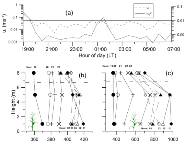
Sonic temperature (Ts) increased with height between 3 and 5 m under low turbulent conditions throughout the night, while increasing turbulence between 20:00 and 07:00 LT shifted theTs gradient from positive to negative with height (Fig. 2). However, at the top of the measured profile, the temperature gradient was nearly zero for u∗< 0.05 ms−1
(Table 3). The mean bulk Richardson number (RB) at the geometric mean height of the top two measurements averaged 2.3 when u∗< 0.05 ms−1. For conditions with u∗>=0.05 ms−1the meanRBwas−1.2. Shifts in wind di-rection above the canopy (5 to 8 m height) were highly vari-able foru∗less than approximately 0.05 ms−1(Fig. 3). These
shifts coincided with vertical wind velocity variance less than 0.01 m2s−2 and the horizontal wind velocity variance less than 0.1 m2s−2(Fig. 3). At these low turbulence conditions, turbulent transport of gases originating at the earth surface is minimal resulting in the accumulation of gases in a layer of air bounded by a cap in the surface boundary layer. The top of the surface-influenced control volume in which mass accumulation was set at 6.3 m (geometric mean of 5 and 8 m; 2.5H) (Fig. 4).
Over the 19:00 to 07:00 LT time frame, the line-averaged concentrations of CO2 at 1 m within the canopy ranged from 354 to 1038 µmol mol−1while point concentrations at 8 m a.g.l. (5.2 m or 2.9Habove the canopy) varied from 358 to 862 µmol mol−1. The difference between the 5 m (1.7H) and 8 m (2.9H) CO2concentrations ranged from−11.4 to 337 µmol mol−1. Eleven percent of the 90 min mean concen-tration gradients at the top of the layer were high enough to calculate a turbulent diffusive flux. The mean CO2 gra-dient (1CO2/1z) was less than or equal to the MDL when u∗> 0.05 ms−1(Table 3).
Over the 19:00 to 07:00h LT time frame, the line-averaged N2O concentrations within the canopy (0.4H) ranged from 0.313 to 0.467 µmol mol−1 while the point sample at 8 m
ranged from 0.295 to 0.448 µmol mol−1. The difference be-tween the 5 m (1.7H) and 8 m (2.9H) N2O concentrations above the canopy ranged from−0.357 to 0.059 µmol mol−1. Twelve percent of the 90 min mean concentration gradients at the top of the layer were high enough to calculate a tur-bulent diffusive flux. The mean N2O gradient (1N2O/ 1z) was less than the MDL whenu∗> 0.05 ms−1(Table 3).
A common feature of the mean concentration profiles of both CO2 and N2O was a lower mean concentration from air sampled at a point 3 m (1.2H) than both the 1 m (0.4H) and 5 m (1.7H) mean concentrations. This may be a result of the close proximity of the 1.2H point measurement to the canopy top representing only local canopy conditions. Conversely, the spatially averaged line concentration in the canopy at 0.4H could better approximate the mean concen-tration at that height within the canopy. Consequently, con-centration measurements at 2.8 m were excluded from all profiles prior to mass integration.
The temporal patterns of mass build-up were similar for N2O and CO2(Fig. 4). The increase in either N2O or CO2 concentrations in the lowest 6.3 m corresponded to a decrease in wind speeds at 8 m (Fig. 2) as well as lowu∗ and
Figure 4.Near-surface atmospheric conditions during the night of 5 August 2015. The friction velocity (u∗, left ordinate) and vertical wind velocity variance (σw2, right ordinate) at 8 m are indicated from 19:00 to 07:00 LT in panel(a). The solid line(a)indicates the upper thresholds for the “low turbulence” classification. Labeled profiles of N2O and CO2concentrations every hour from 19:00 until 03:00 LT are indicated with differing symbols and lines in panels b and c. Note the 01:00–02:00 LT burst of vertical wind variance(a)corresponds to losses in N2O(b)and CO2(c). Sunrise and sunset times were approximately 07:00 and 21:00 LT.
Figure 5.Mean profiles of wind speed, sonic temperature, and concentrations of CO2and N2O under different friction velocity and time domain classes for the entire study period. The mean wind speed (U, panela), sonic temperature (Ts; panelb), and concentration profiles of CO2(c)and N2O(d)when the air at 8 m had low turbulence (u∗≤0.05 ms−1) or turbulent (u∗>0.05 ms−1) between 19:00 and 03:00 LT and 03:00 and 07:00 LT are indicated. Canopy height was 2.8 m. Smaller symbols not connected with lines represent concentration measurements excluded from mass accumulations due to their close proximity to the canopy top.
On average, the mean profiles of CO2 and N2O concen-trations during from 19:00 to 03:00 LT showed nearly iden-tical concentrations at 1 and 5 m with decrease in concen-tration at 8 m (Fig. 5). The corresponding mean concentra-tion profiles for the 03:00 to 07:00 LT time window showed
no change in concentration with height (Fig. 5). Conditions during the 19:00 to 03:00 LT period resulted in nearly iden-tical mean wind speed profiles regardless ofu∗but
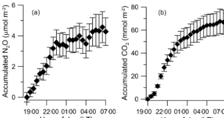
Figure 6.Accumulation of CO2and N2O within the lowest 6.3 m of the boundary layer during the night throughout the study period. The mean accumulations of N2O(a) and CO2 (b) are indicated with vertical error bars, indicating the standard error of the mean of each 30 min mean accumulation. Sunrise was approximately 06:00 to 07:00 LT.
between 19:00 and 03:00 LT regardless ofu∗(Fig. 5). The
temperature inversion was also evident between 03:00 and 07:00 LT when u∗ was less than 0.05 ms−1 (Fig. 5). This
near-surface inversion was not evident at the top of the accu-mulation control volume (between 5 m and 8 m a.g.l.) where the wind shear was high.
3.2 Mass accumulations
Using the previously defined top of the accumulation con-trol volume, the accumulations of N2O and CO2were often evident during the night from 19:00 to 00:00 LT with sunset approximately 21:00 LT (Fig. 6). These mass accumulations corresponded to positivez/3(locally stable conditions) and low u∗ (low turbulence). After quality assurance of the
ac-cumulated flux calculations, there were 97 90 min measure-ments of N2O nocturnal flux and 78 90 min measurements of CO2nocturnal flux withu∗less than 0.05 ms−1. Note that the
mean gradients of both N2O and CO2were less for this set of measurements (Table 4) than for all measurement periods (Table 3).
Accumulated N2O flux during low turbulence and no mea-surable diffusive flux across the control volume top aver-aged 0.22 nmol m−2s−1 with a variability (standard devi-ation) greater than the mean (Table 4). The accumulated fluxes of N2O between 19:00 and 03:00 LT were relatively steady over the measurement period (Fig. 8). Accumulations within the control volume were greater (0.58 nmol m−2s−1)
during the 22 % of the measured flux periods when there was measurable diffusive flux out the top of the control vol-ume (Table 4). When measurable, the diffusive flux of N2O was twice the accumulative flux (Table 4), resulting in a mean total measured N2O flux (accumulative+diffusive) of 0.53 nmol m−2s−1(SD=0.25 nmol m−2s−1). This suggests that the ability to estimate diffusion across the upper bound-ary was limited by the N2O gradient. These fluxes were sim-ilar to median daily flux gradient-derived fluxes for maize
T able 4. Flux of N2 O and CO 2 across the top of the accumulation control v olume during stable (positi v e local Ob ukho v length) nocturnal conditions between 19:00 and 07:00 L T . Accumulation flux based on 90 min mass accumula tions. Dif fusi v e flux based on av erage of 3 half-hour gradients. Flo w condition Statistic Gradient at top of control N2 O accumulation flux N2 O dif fusi v e flux CO 2 accumulation flux CO 2 dif fusi v e flux at 8 m v olume (6.3 m a.g.l.) (nmol m − 2s − 1) (nmol m − 2s − 1) (µmol m − 2s − 1) (µmol m − 2s − 1) N2 O CO 2 without measurable with measurable without measurable with measurable (µmol m − 4) (mmol m − 4) dif fusion dif fusion dif fusion dif fusion Lo w turb ulence Mean 0.04 0.43 0.22 0.58 1.06 0.40 0.37 3.33 u
a≤∗
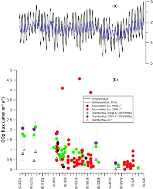
Figure 7.Temperatures and CO2flux based on accumulation and chamber methods. Diurnal variation in air (solid black line) and 10 cm soil at 10 cm depth (dashed blue line) during the period are indicated in panel a. Total fluxes (accumulative within and diffusive out the top of the control volume) under stable, low turbulence conditions and soil+root fluxes calculated using the chamber method are indicated in panel(b) (ordinate axis with differing units to left and right). The standard deviation of the three chamber flux measurements in each field is indicated by the vertical bars.
grown over 2 years in a similar climate (Ontario, Canada) on imperfectly drained silt-loam soils with conventional tillage (0.5 nmol m−2s−1)but lower than that for no-till (Wagner-Riddle et al., 2007, Table 1).
The accumulated CO2fluxes between 19:00 and 03:00 LT generally decreased over time with values ranging from approximately 2.0 to 0.2 µmol m−2s−1 (Fig. 7). The mass accumulative flux during low turbulence averaged 0.40 µmol m−2s−1 with a variability less than the mean (Table 4). Measurable diffusive CO2 flux out of the con-trol volume, occurring 23 % of the low turbulence CO2 flux events, corresponded to only slightly lower accumu-lative fluxes (0.37 µmol m−2s−1; Table 4). This suggested that the limiting factor in estimating diffusion across the control volume was the turbulent exchange process not the
concentration gradient. When measurable, the diffusive flux of was 9 times the accumulative flux (Table 4), result-ing in a mean total measured CO2 flux (accumulative + diffusive) of 1.16 µmol m−2s−1. (SD=0.49 µmol m−2s−1). This flux was substantially lower than eddy-covariance-derived nocturnal mean flux over maize fields (10.8 to 30.0 µmol m−2s−1) in a similar climate (Ontario, Canada) during the same period in the growing season but under more turbulent winds: mean wind speeds of at least 1.5 ms−1and
u∗ between 0.075 and 0.1 ms−1 (Pattey et al., 2002)
com-pared to mean wind speeds of 1.1 ms−1andu
∗of 0.02 ms−1.
Greater turbulence (higheru∗at 8 m) did not affect the
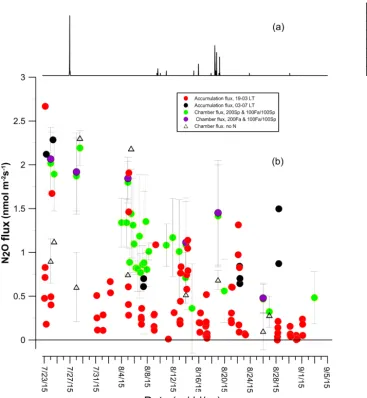
Figure 8.Precipitation and N2O flux based on accumulation and chamber methods. Precipitation is indicated in panel(a). Total fluxes (accumulative within and diffusive out the top of the control volume) under stable, low turbulence conditions and soil+root fluxes calculated using the chamber method are indicated in panel(b)(ordinate axis with differing units to left and right). The standard deviation of the three chamber flux measurements in each field is indicated by the vertical bars.
accumulative CO2flux whether or not there was measurable diffusion (Table 4). The greater turbulence corresponded to a decrease in the mean N2O gradient and an increase in the CO2gradient at the top of the control volume and increased diffusive flux out of the control volume (Table 4). The upper transport cap to the mass accumulation control volume was on average stronger for the low turbulence condition than the higher turbulence condition (based on σw and σw/u∗;
Ta-ble 2) and the eddy diffusivities were lower (TaTa-ble 3). The effectiveness of this cap, separating the developing nocturnal boundary layer above from the surface boundary layer below, had a larger effect on the mass accumulation of CO2 than N2O and a greater effect on the diffusive flux of N2O than CO2(Table 4). This might be expected if the local CO2flux was more similar to the more distant surroundings (more
ho-mogeneous) than the N2O flux. It is important to note, how-ever, that the high variability in CO2and N2O fluxes under low turbulence resulted in mean accumulative fluxes with or without measurable diffusive flux that was not statistically different (Studentttest;p=0.05) (Table 4).
Eddy diffusivities were comparable to and exhibited the same relationship to u∗ and z/3 for positive z/3 as
those reported for N2O and NH3 in Schäfer et al. (2012). The mean eddy diffusivities were more than an order of magnitude higher for conditions with u∗>0.05 ms−1
thanu∗≤0.05 ms−1 (Table 3). Clearly theu∗ threshold of
diffu-sive versus accumulative flux (Table 4) during low turbulence conditions, however, may also be a result of a combination of non-stationarity of the flow and/or anemometer tilt. Assum-ing stationary flow and no anemometer tilt, the approxima-tion of the eddy diffusivities of N2O and CO2by substituting molecular Schmidt numbers for turbulent Schmidt numbers likely contributed to underestimated flux values since these Schmidt numbers were higher than the generalized turbulent Schmidt number of Flesch et al. (2002).
3.3 Soil chamber fluxes
The soil chamber CO2and N2O flux measurements, made at various hours of the day during the measurement period, also showed a decreasing flux over the period (Figs. 7, 8). CO2 flux in the 200Sp treatment, where the profile measurements were made, ranged from 0.1 to 2.1 µmol m−2s−1and aver-aged 0.9 µmol m−2s−1. These chamber measurements had a mean signal-to-noise ratio of 250. These fluxes are similar to soil+root respiration fluxes reported in the literature for maize fields (Table 1). The region of the south field in which no N was applied during the past year (Fig. 1) had a mean CO2 emission of 0.5 µmol m−2s−1, averaging 50 % of the mean field emissions under various N treatments and similar to that reported for soil+root respiration of soybean in the lit-erature (Table 1). Although most measurements were made at 23:00 LT, some of the variability in chamber measurements was a result of the time of measurement. The 4-day study of diurnal variation in mean hourly CO2 emissions ranged from 1.04 to 1.48 µmol m−2s−1 with the highest emissions at 18:00 LT with a ratio of midnight-to-noon LT emissions of 1.2.
Nitrous oxide fluxes in the 200Sp treatment field ranged from 0.3 to 2.2 nmol m−2s−1, averaging 1.1 nmol m−2s−1. These fluxes were lower than commonly reported in the lit-erature for maize but similar to that of soybeans (Table 1). This may be due to the negligible amount of the applied nitrogen available for denitrification and nitrification in the maize field. These chamber N2O measurements thus had a mean signal-to-noise ratio of 1.7. The fields on which no N was applied during the year had a mean emission of 0.59 nmol m−2s−1, 54 % of the mean fertilized field emis-sions and equal to the Chamber method MDL. As with the CO2flux measurements, some of the variability in chamber measurements was a result of the time of measurement. The 4-day study of diurnal variation in mean hourly N2O emis-sions ranged from 0.96 to 1.40 nmol m−2s−1with the high-est emissions at 18:00 LT with a ratio of midnight-to-noon LT emissions of 0.93.
3.4 Comparative fluxes
As with the comparison of CO2 fluxes determined by eddy covariance and boundary layer mass balance (Eugster and Siegrist, 2000), the fluxes determined by chamber and mass
accumulation are local and regional fluxes, respectively. The CO2flux measurements based on mass accumulation within the control volume but not diffusion across the control vol-ume top were generally lower than the chamber measure-ments, with the exception of a few outlying high mass ac-cumulation values (Fig. 7). Inclusion of measurable diffusive flux to the accumulative flux resulted in total flux estimates more similar to soil chamber measurements. Average mean daily CO2 flux estimates for two of the three measurement time periods indicated the total mass accumulation method flux was between 0.9 and 1.3 of that determined by the cham-ber method (Table 5). Higher accumulation flux over the chamber flux was expected because the chamber flux method measured only root and soil respiration while the mass accu-mulation flux method measured the respiration of the soil, roots, stalks, and leaves. This can result in a large difference in flux: Parkin et al. (2005) measured soil and root respiration with chambers and whole canopy respiration by eddy covari-ance and found that the soil respiration was approximately 50 % of the total measured CO2 flux. Given the variability in daily flux estimates within each period, the fluxes deter-mined by chamber and mass accumulation methods were not significantly different (Table 5).
The N2O flux measurements based on mass accumulation under low turbulence and stable conditions were generally much lower than those measured using the chambers on the same day (Fig. 8). Inclusion of measurable diffusive fluxes in the flux estimates over three measurement time periods showed that the accumulation method estimated mean daily fluxes only 60 to 80 % of the soil chambers (Table 5). Again, given the variability in mean daily flux estimates within each time period, the fluxes determined by the chamber and mass accumulation methods were not significantly different (Ta-ble 5).
Differences between the accumulation flux versus cham-ber flux measurements were likely in part due to the advec-tion of gas emitted from surrounding fields. The accumulated mass of CO2 and N2O have contributions from local soils sources as well as mass advection from more distant sources due to the meandering nature of the air flow during the stable nocturnal conditions (Eugister and Siegrist, 2000). Unfortu-nately, the analytical approaches to defining the flux foot-print do not apply to the stable nocturnal conditions in which the accumulations occur (z/3>+1,u∗< 0.05 ms−1; Vesala
et al., 2007), although they are believed to be on the order of 10 km (e.g., Chambers et al., 2011). At scales of kilometers (10 km2area), the land use was crop agriculture, dominated by nearly equal soybean and maize production (46 and 47 %, respectively, with an addition 2 % in grass in the Table 1). Within the nearest square kilometer around the research site, maize production dominated the land use (Table 1).
(Ta-Table 5.Comparative mean daily fluxes of N2O and CO2across three similar flux periods.
Total mass accumulation flux Chamber flux in Sp200 Ratio
(including accumulative and treatment field diffusive flux when measurable)
Measurement period n∗ Mean Standard n∗ Mean Standard Mass accumulation/
(DD/MM/YY) deviation deviation Chamber
CO2 No. µmol m−2s−1 µmol m−2s−1 No. µmol m−2s−1 µmol m−2s−1
22/07/15–31/07/15 – – – 2 1.60 0.37 –
01/08/15–22/08/15 12 0.76 0.60 11 0.83 0.44 0.9
23/08/14–2/09/15 4 0.21 0.08 2 0.16 0.10 1.3
N2O No. nmol m−2s−1 nmol m−2s−1 No. nmol m−2s−1 nmol m−2s−1
23/07/15–31/07/15 5 1.20 0.83 2 1.93 0.34 0.6
01/08/15–22/08/15 14 0.76 0.18 11 1.00 0.35 0.8
23/08/14–10/09/15 7 0.25 0.15 2 0.40 0.22 0.6
∗Number of days with valid measurements.
ble 1). If anything, it is reasonable to assume that the ad-vected, regionally emitted CO2 from surrounding soybean and maize production would have increased the accumula-tion flux estimates. However, the relatively low accumulaaccumula-tion fluxes suggest that advection did not substantially contribute to the measured mass accumulation. The measured cham-ber N2O flux from unfertilized fields of maize was typically lower than fertilized maize fields and closer to the flux mea-sured by the accumulation method (Fig. 8). Since roughly one-half the surrounding area was in soybean production (Ta-ble 1), it is reasona(Ta-ble to assume horizontal advection of air with higher N2O concentration from nearby grass and soy-bean canopies could have potentially affected the N2O pro-file. However, literature values for fluxes from surrounding grassy areas and soybean fields (Table 1) are generally simi-lar to the flux measured by the accumulation method in a fer-tilized maize field (Table 5). Consequently there is little ev-idence to support the supposition that advection contributed significantly to the accumulated mass.
The general underestimate of CO2and N2O fluxes using the mass accumulation method may also be a result of using two small of an accumulation volume. The cap of the volume was arbitrarily set at the geometric mean between the upper two measurement heights. An objective measure of the cap height is needed. Given the significantly greater flux associ-ated with diffusion out the top of the accumulation control volume relative to the computed accumulated flux within the control volume (Table 4), the accumulation control volume was likely too shallow.
4 Conclusions
Nocturnal CO2 and N2O emissions from the soil surface were determined by measuring the accumulation of mass
within a mixing-limited surface boundary layer control vol-ume and the diffusion of mass out the top of the control volume. The magnitude of the accumulations influenced the ability for the accumulation method to be effective at estimat-ing nocturnal flux: CO2fluxes determined by the accumula-tion method were comparable to those measured using the chamber method while those for N2O were below those mea-sured using the chamber method. For the N2O fluxes, there is no known canopy flux of N2O and consequently the chamber method and accumulation method should have been compa-rable. Measurement errors associated with a limited vertical dimension to the control volume, non-stationarity of low tur-bulent flow in the stable nocturnal surface boundary layer, and estimation of the Schmidt number for the diffusive flux component likely contributed to the differences between the accumulation and chamber flux methods. Advection during the stable nocturnal conditions did not appear to contribute to the measured profiles and the subsequent estimate of N2O flux or CO2flux. Additional work is needed to evaluate the use of the accumulation method for N2O fluxes for accumu-lations within a larger vertical domain to the control volume and more homogeneous regional land use in conjunction with using chamber methods with a lower MDL (higher signal-to-noise ratio).
Author contributions. RHG designed, conducted, and analyzed the
mass accumulation experiment while RAO conducted the chamber gas flux measurements. RHG prepared the manuscript with contri-butions from RAO.
Competing interests. The authors declare that they have no conflict
Acknowledgements. The authors appreciate the field technical assistance of Cheng Hsien Lin and Austin Pearson.
Edited by: Christof Ammann
Reviewed by: three anonymous referees
References
Acevedo, O. C., Moraes, O. L., DaSilva, R., Fitzjarrald, D. R., Sakai, R. K., Staebler, R. M., and Czikowsky, M. J.: Inferring nocturnal surface fluxes from vertical profiles of scalers in an Amazon pasture, Glob. Change Biol., 10, 886–894, 2004. Acevedo, O. C., DaSilva, R., Fitzjarrald, D. R., Moraes, O. L.,
Sakai, R. K., and Czikowsky, M. J.: Nocturnal vertical CO2 ac-cumulation in two Amazonian ecosystems, J. Geophy. Res., 113, G00B004, https://doi.org/10.1029/2007JG000612, 2008. Aubinet, M., Feigenwinter, C., Heinesch, B., Laffineur, Q.,
Pa-pale, D., Reichstein, M., Rinne, J., and van Gorsel, E.: Night-ime flux correction, chap. 5, in: Eddy Covariance: A Practical Guide to Measurements and Data Analysis, edited by: Aubinet, M., Vesala, T., and Paple, D., Springer Atmospheric Sciences, 133–172, https://doi.org/10.1007/978-94-007-2351-1_5, 2012. Biraud, S., Ciais, P., Ramonet, M., Simmonds, V. K., Monfrey, P.,
O’Doherty, S., Spain, G., and Jennings, S. G.: Quantification of carbon dioxide, methane, nitrous oxide and chloroform emis-sions over Ireland from atmospheric observations at Mace Head, Tellus, 54B, 41–60, 2002.
Bowden, R. D., Rullo, G., Stevens, G. R., and Steudler, P. A.: Soil fluxes of carbon dioxide, nitrous oxide and methane at a produc-tive temperate deciduous forest, J. Environ. Qual., 29, 268–276, 2000.
Bremner, J. M., Robbins, S. G., and Blackmer, A. M.: Seasonal vari-ability in emissions of nitrous oxide from soil, Geophys. Res. Lett., 7, 641–644, 1980.
Bremner, J. M., Breitenbeck, G. A., and Blackmer, A. M.: Effect of anhydrous ammonia fertilization on emission of nitrous oxide from soils, J. Environ. Qual., 10, 77–80, 1981.
Chamber, S., Williams, A. G., Zahorowski, W., Griffiths, A., and Crawford, J.: Separating remote fetch a local mixing influences on vertical radon measurements in the lower atmosphere, Tellus, 63B, 843–859, 2011.
De Costa, J. M. N., Rosenberg, N. J., and Verma, S. B.: Respiratory release of CO2in alfalfa and soybean under field conditions, Agr. Forest Meteorol., 37, 143–158, 1986.
Draxler, R. R. and Hess, G. D.: An overview of the HYSPLITY-4 modelling system for trajectories, dispersion, and depositio, Aust. Meteorol. Mag., 47, 295–308, 1998.
Duxbury, J. M. and Bouldin, D. R.: Emissions of nitrous oxide from soils, Nature (London), 298, 462–262, 1982.
Eichner, M. J.: Nitrous oxide emissions from fertilized soils: sum-mary of available data, J. Environ. Qual., 19, 272–280, 1990. Eugster, W. and Siegrist, F.: The influence of nocturnal CO2
advec-tion on CO2flux measurements, Basic Appl. Ecol., 1, 177–188, 2000.
Flesch, T. K., Prueger, J. H., and Hatfield, J. L.: Turbulent Schmidt number from a tracer experiment, Agr. Forest Meteorol., 111, 299–307, 2002.
Foken, T., Goeckede, M., Mauder, M., Mahrt, L., Amiro, B., and Munger, W.: Post field data quality control, in: Handbook of Mi-crometeorology, edited by: Lee, X., Massman, W., and Law, B., Kluwer Academic Pub, Dordrecht, the Netherlands, 181–208, 2004.
Goodroad, L. L., Keeney, D. R., and Peterson, L. A.: Nitrous oxide emissions from agricultural soils in Wisconsin, J. Environ. Qual., 13, 557–561, 1984.
Grant, R. H. and Boehm, M. T.: Manure ammonia and hydrogen sulfide emissions from a western dairy storage basin, J. Environ. Qual., 44, 1–10, 2015.
Kaimal, J. C. and Finnigan, J. J.: Atmospheric Boundary Layer Flows: their structure and measurement, Oxford Univ. Press, NY, USA, 289 pp., 1994.
Lee, X., Black, T. A., den Hartog, G, Neumann, H. H., Nesic, Z., and Olejnik, J.: Carbon dioxide exchange and nocturnal pro-cesses over a mixed deciduous forest, Agr. Forest Meteorol., 81, 13–29, 1996.
Lee, X., Finnigan, J., and Paw U, K. T.: Coordinate systems and flux bias error, in: Handbook of Micrometeorology, edited by: Lee, X., Massman, W., and Law, B., Kluwer Academic Pub, Dor-drecht, the Netherlands, 33–66, 2004.
Mahrt, L.: The near-calm stable boundary layer, Bound.-Lay. Mete-orol., 140, 343–360, 2011.
Massman, W. J.: A review of the molecular diffusivities of H2O, CO2, CH4, CO, O3, SO2, NH3, N2O, NO, and NO2in air, O2 and N2near STP, Atmos. Environ., 32, 111–1127, 1998. Mosier, A., Shimel, D., Valentine, D., Bronson, K., and Parton, W.:
Methane and nitrous oxide fluxes in native, fertilized and culti-vated grasslands, Nature, 350, 330–332, 1991.
Mosier, A. R., Halvorson, A. D., Reule, C. A., and Liu, X. J.: Net Global Warming Potential and Greenhouse Gas Intensity in Ir-rigated Cropping Systems in Northeastern Colorado, J. Environ. Qual., 35, 1584–1598, 2006.
Omonode, R. A., Vyn, T. J., Smith, D. R., Hegymegi, P., and Gal, A.: Soil carbon dioxide and methane fluxes from long-term tillage systems in continuous corn and corn-soybean rotations, Soil Till. Res., 92, 182–195, 2007.
Parkin, T. B. and Kaspar, T. C.: Nitrous oxide emissions from corn-soybean systems in the Midwest, J. Environ. Qual., 35, 1496– 1506, 2006.
Parkin, T. B., Kaspar, T. C., Sennwo, Z., Prueger, J. H., and Hatfield, J. L.: Relationship of soil respiration to crop and landscape in the Walnut Creek watershed, J. Hydromet., 6, 812–824, 2005. Pattey, E, Strachan, I. B., Desjardins, R. L., and Massheder, J.:
Mea-suring CO2flux over terrestrial ecosystems using eddy covari-ance and nocturnal boundary layer methods, Agr. Forest Meteo-rol., 113, 145–158, 2002.
Pendall, E., Schwendenmann, L., Rahn, T., Millers, J. B., and Tans, P. P.: Land use and season affect fluxes of CO2, CH4, CO, N2O, H2and isotopic source signatures in Panama: evidence from noc-turnal boundary layer profiles, Glob. Change Biol., 16, 2721– 2736, 2010.
Raich, J. W. and Tufekcioglu, A.: Vegetation and soil respiration: correlations and controls, Biogeochem., 48, 71–90, 2000. Schäfer, K., Grant, R. H., Emeis, S., Raabe, A., von der Heide,
bound-ary layer conditions, Atmos. Meas. Tech., 5, 1571–1583, https://doi.org/10.5194/amt-5-1571-2012, 2012.
Tufekcioglu, A., Raich, J. W., Isenhart, T. M., and Schultz, R. C.: Soil respiration within riparian buffers and adjacent fields, Plant Soil, 229, 117–124, 2001.
USDA: Cropscape – Cropland Data Layer, Center for Spatial In-formation Science and Systems, National Agricultural Statis-tics Service, United States Department of Agriculture, available at: https://nassgeodata.gmu.edu/CropScape/, last access: 15 June 2017.
van de Wiel, B. J. H., Moene, A. F., De Ronde, W. H., and Jonker, H. J. J.: Local similarity in a stable boundary layer and mixing-length approaches: consistency of concepts, Bound.-Lay. Meteo-rol., 128, 103–116, 2008.
Vesala, T., Kljun, N., Rannik, Ü., Rinne, J., Sogachev, A., Markkan, T., Sabelfeld, K., Foken, Th., and Lecelerc, M. Y.: Flux and con-centration footprint modelling: State of the art, Envon. Poll., 152, 653–666, https://doi.org/10.1016/j.envpol.2007.06.070, 2007. Wagner-Riddle, C., Furon, A., McLaughlin, N. L., Lee, I., Barbeau,
J., Jayasundrara, S., Parkin, G., and von Bertold, P.: Intensive measurement of nitrous oxide emissions from a corn-soybean-wheat rotation under two contrasting management systems over 5 years, Glob. Change Biol., 13, 1722–1736, 2007.