and its Applications
I. Elbatal
Department of Mathematics and Statistics, College of Science Al Imam Mohammad Ibn Saud Islamic University, Saudi Arabia iielbatal@imamu.edu.sa
Yehia M. El Gebaly
Department of Statistics, Mathematics and Insurance Benha University, Egypt
yehia1958@hotmail.com
Essam A. Amin
Department of Mathematics and Statistics, College of Science Al Imam Mohammad Ibn Saud Islamic University, Saudi Arabia Institute of Statistical Studies and Research
Department of Mathematical Statistics, Cairo University, Egypt eaabdelsamad@imamu.edu.sa
Abstract
A new six-parameter distribution called the beta generalized inverse Weibull-geometric distribution is proposed. The new distribution is generated from the logit of a beta random variable and includes the generalized inverse Weibull geometric distribution. Various structural properties of the new distribution including explicit expressions for the moments, moment generating function, mean deviation are derived. The estimation of the model parameters is performed by maximum likelihood method.
Keywords: Generalized Inverse Weibull, Geometric distribution, Beta-G, Moments, Reliability Function, Maximum Likelihood.
1. Introduction
The inverse Weibull (IW) distribution has many applications in the reliability engineering discipline and model degradation of mechanical components such as the dynamic components (pistons, crankshafts of diesel engines, etc). It provides a good fit to several data such as the times to breakdown of an insulating fluid, subject to the action of constant tension. Also, it can be used to model a variety of failure characteristics such as infant mortality, useful life and wear-out periods, applications in medicine and ecology, determining the cost effectiveness, maintenance periods of reliability centered maintenance activities. Keller et al. (1985) obtained the IW model by investigating failures of mechanical components subject to degradation. de Gusmão et al. (2011) introduced the three-parameter generalized IW (GIW) distribution with decreasing and unimodal failure rate.
The cumulative distribution function (cdf) and probability density function (pdf) of the GIW distribution are defined (for ) by
Recently, there have been many attempts to define new families of probability distributions that extend well-known families of distributions and at the same time provide great flexibility in modeling data in practice. One such class of distributions generated by compounding the well-known lifetime distributions such as exponential, Weibull (W), generalized exponential and exponentiated W with the geometric (Gc) distribution. For example, Adamidis and Loukas (1998) introduced the exponential-geometric (EGc), Barreto-Souza et al. (2010) pioneered the Weibull-exponential-geometric (WGc) and Adamidis et al. (2005) proposed the extended exponential-geometric (EEGc) distributions.
Let be a geometric random variable with probability mass function given by
(2)
In this paper, we define and study a new lifetime model called the beta generalized inverse Weibull geometric (BGIWGc) distribution. Its main characteristic is that three additional shape parameters are added in Equation (1) to provide more flexibility for the generated distribution. Based on compounding the GIW distribution with the Gc distribution and then using the beta-G (B-G) family pioneered by Eugene et al. (2002), we construct the six-parameter BGIWGc model and give a comprehensive description of some of its mathematical properties. We aim that it will attract wider applications in engineering, medicine and other areas of research.
At first, we will define the GIW-geometric (GIWGc) distribution and then we use the B-G to construct the BB-GIWB-Gc model.
Suppose that a company has systems functioning independently and producing a certain product at a given time, where is a random variable, which is often determined by economy, customers demand, etc. The reason for considering as a random variable comes from a practical viewpoint in which failure (of a device for example) often occurs due to the present of an unknown number of initial defects in the system. Let has the pmf in (geometric).
Now, consider the failure times of the initial defects, denoted by be independent and identically distributed (iid) random variables following the GIW distribution with cdf and pdf (1). Note that the time to failure of the first out of the functioning systems is given by { } Then, the cdf of is given (for ) by
* + (3)
where and
The corresponding pdf of the new model can be written as
, *
Henceforth, we denote a random variable having pdf (4) by GIWGc .
The survival function (sf) and hazard rate function (hrf) of the GIWGc distribution are given by
and
[ ][ ]
For an arbitrary baseline cdf the B-G family due to Eugene et al. (2002) has the cdf and pdf given (for ) by
∫
(5)
where and are two additional parameters whose role is to introduce skewness and to vary tail weight and
is the incomplete beta function with and is the
incomplete beta function ratio. One major benefit of this class of distributions is its ability of fitting skewed data that cannot be properly fitted by existing distributions. If
, and then is usually called the exponentiated distribution (or the Lehmann type-I distribution). Indeed, if is a beta distributed random variable with parameters and , then the cdf of agrees with the cdf given in (5).
The B-G has the following special cases
• If is the cdf of a standard uniform distribution, the cdf (5) yields the cdf of the beta distribution with parameters and .
• If is an integer value and , then the cdf (5) becomes
∫
∑ ( ) [ ][ ]
which is really the cdf of the order statistic of a random sample of size from distribution .
• For , then the cdf (5) reduces to . • The cdf (5) reduces to [ ] , for
For general and , the cdf (5) can be defined in terms of the well-known hypergeometric function by
( )
where
∑
| |
where denotes the ascending factorial of . We
obtain the properties of for any B-G distribution defined from a parent in (5) could, in principle, follow from the properties of the hypergeometric function which are well established in the literature; see, for example, Section 9.1 of Gradshteyn and Ryzhik (2000).
The pdf and hrf of the B-G class are given by
{ } (6)
and
{ }
[ ]
respectively, where [ ] is the survival function of the B-G distribution.
The B-G class has been used to construct various extensions for the well-known distributions. For example, the beta normal (Eugene et al., 2002), beta Fréchet (Nadarajah and Gupta, 2004), beta exponential (Nadarajah and Kotz, 2006), beta W (Lee et al., 2007), beta W-geometric (Cordeiro et al., 2011), beta generalized exponential (Barreto-Souza et al., 2010), beta modified W (da Silva et al., 2010), beta IW (BIW) (Khan, 2010), beta exponential-geometric (Bidram, 2012) and beta exponential Fréchet (Mead et al., 2017) distributions.
2. The BGIWGc distribution
In this section, we difine the six parameter BGIWGc distribution by inserting (3) in equation (5). Then, the cdf of the BGIWGc distribution is given by
∫
(7)
where and are shape parameters. The random variable with the cdf (7) is said to have a BGIWGc distribution and will be denoted by BGIWGc where
.
The corresponding pdf of (7) takes the form
( )
* ( )+ (8)
The hazard (failure) rate function (hrf) of is given by
*
+
{ [ ]}
[ ]
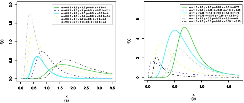
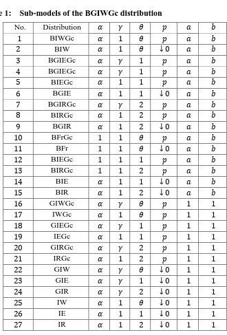
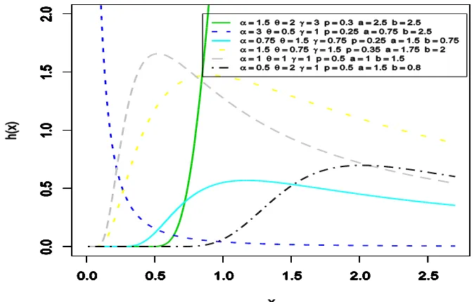
The BGIWGc distribution is a very flexible model that approaches to different distributions when its parameters are changed. Its 27 sub-models are listed in Table 1. Figure 1 displays some plots of the BGIWGc pdf for some values and the plots of its hrf are shown in Figure 2.
3. Linear representation
In this subsection we present a useful linear representation for the BGIWGc pdf. Consider the series expantion given, for | | and is a positive real non-integer, by
∑
(9)
Applying (9) to Equations (8), we can write
∑
∑ (
)
Table 1: Sub-models of the BGIWGc distribution
No. Distribution
BIWGc
BIW
BGIEGc
BGIEGc
BIEGc
BGIE
BGIRGc
BIRGc
BGIR
BFrGc
BFr
BIEGc
BIRGc
BIE
BIR
GIWGc
IWGc
GIEGc
IEGc
GIRGc
IRGc
GIW
GIE
GIR
IW
IE
Figure 2: Hrf plots of the BGIWGc distribution for selected values of the parameters
Using the series representation
∑
| |
(10)
The last pdf can be expressed, after applying (10), as
∑
( )
(11)
where is the pdf of the BGIW distribution with parameters
and . Equation (11) reveals that the BGIWGc dnsity function can be expressed as an infinite linear mixture of BGIW densities. Hence, we can obtain some mathematical properties of the BGIWGc distribution from those properties of the BGIW distribution.
3. Properties
In this section, we study the statistical properties of the BGIWGc distribution including ordinary and incomplete moments and moment generating function.
3.1 Ordinary and incomplete moments
Lemma (3.1): If has BGIWGc where then the moment of
. has the following form:
∑ [ ]
(12)
where
∑
( )
Proof.
Let be a random variable with density function (8). The th ordinary moment of the BGIWGc distribution is given by
∫
∑ ( )
∫
∑ ( )
[ ]
∑
[ ]
which completes the proof.
Lemma (3.2): If has BGIWGc , then the moment generating function has the following form
∑
[ ] (13)
Proof.
We start with the well known definition of the moment generating function given by
∫ Since ∑
converges and each term is integrable for all close to , then we can rewrite the moment generating function as
∑ by replacing . Hence using (12) the MGF of BGIWGc distribution is given by
∑
[ ]
which completes the proof .
Similarly, the characteristic function of the BGIWGc distribution becomes
3.2 Conditional moments
For lifetime models, it is also of interest to find the conditional moments and the mean residual lifetime function. The conditional moments for BGIWGc distribution is given by the following Lemma.
Lemma (3.3): If has BGIWGc , the conditional moments for BGIWGc distribution is given by
| ∑ [
[ ] ]
Proof.
| ∫
∑ ( )
∫
∑ [
[ ] ]
where ∫ is the upper incomplete gamma function.
The mean residual lifetime function of beta additive Weibull distribution is given by
|
∑ [
[ ] ]
The importance of the MRL function is due to its uniquely determination of the lifetime distribution as well as the hrf.
3.3 Residual and reversed residual functions
Given that a component survives up to time , the residual life is the period beyond until the time of failure and defined by the conditional random variable | . In reliability, it is well known that the mean residual life function and ratio of two consecutive moments of residual life determine the distribution uniquely. Therefore, the
th-order moment of the residual lifetime can be obtained via the general formula
| ∫
Applying the binomial expansion of into the above formula, we have
∑ ∑ ( )
∫
∑ ∑ (
On the other hand, we analogously discuss the reversed residual life and some of its properties. The reversed residual life can be defined as the conditional random variable
| which denotes the time elapsed from the failure of a component given that its life is less than or equal to .
The th-order moment of the reversed residual life can be obtained as
|
∫
Using (8) and applying the binomial expansion of , we can write
∑ ∑ ( )
∫
∑ ∑ ( )
[ ]
where ∫ is the lower incomplete gamma function.
3.4 Mean deviations and Bonferroni and Lorenz curves
The mean deviation about the mean and mean deviation about the median measure the amount of scatter in a population. For random variable with pdf , cdf , mean
and Median , the mean deviation about the mean and mean deviation about the median are, respectively, defined by
∫ | | ∫
and
∫ | | ∫
Then, for , we have
∫ ∑ [
[ ] ]
and
∫ ∑ [
[ ] ]
The Bonferroni and Lorenz Curves have applications not only in economics to study income and poverty, but also in other fields like reliability, demography, insurance and medicine. The Bonferroni and Lorenz curves are defined by
∫ ∑ [
[ ] ]
and
∫ ∑ [
[ ] ]
4. Maximum likelihood estimation
In this section, we determine the maximum likelihood estimates (MLEs) of the parameters of the BGIWGc distribution from complete samples only. Let be a random sample of size from the BGIWGc distribution given by (8).
The total log-likelihood function for , where , is given by
∑
∑
∑
(
)
∑
* (
)+
The log-likelihood can be maximized either directly by using the SAS program or R-language or by solving the nonlinear likelihood equations obtained by differentiating the last equation.
The components of the score function ( ) are
∑ ∑
∑
∑ ( ) * ( )+
∑ ∑ ∑
∑
( )
∑
(
∑
∑
( )
∑
[ ( )]
∑
( )
[ ( )]
∑ * (
)+
and
∑ (
)
The maximum likelihood estimation (MLE) of , say ̂ , is obtained by solving the nonlinear system . These equations cannot be solved analytically, and statistical software can be used to solve them numerically via iterative methods. We can use iterative techniques such as a Newton-Raphson type algorithm to obtain the estimate
̂. For interval estimation and hypothesis tests on the model parameters, we require the information matrix.
Applying the usual large sample approximation, MLE of , i.e ̂ can be treated as being approximately , where [ ]. Under conditions that are fulfilled for parameters in the interior of the parameter space but not on the boundary, the asymptotic distribution of √ ̂ is , where = is the unit information matrix. This asymptotic behavior remains valid if is replaced by the average sample information matrix evaluated at ̂, say ̂ . The estimated asymptotic multivariate normal ̂ distribution of ̂ can be used to construct approximate confidence intervals for the parameters and for the hazard rate and survival functions. An asymptotic confidence interval for each parameter is given by
. ̂ √ ̂ ̂ √ ̂/
where is the upper percentile of the standard normal distribution.
5. Data analysis
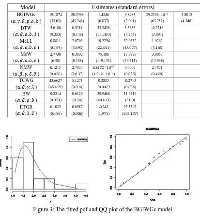
The data set (Gross and Clark, 1975, page 105) on the relief times of twenty patients receiving an analgesic is: 1.1, 1.4, 1.3, 1.7, 1.9, 1.8, 1.6, 2.2, 1.7, 2.7, 4.1, 1.8, 1.5, 1.2, 1.4, 3, 1.7, 2.3, 1.6, 2. For these data, we compare the fits of the BGIWGc distribution with the beta transmuted W (BTW) (Afify et al., 2017), McDonald log-logistic (McLL) (Tahir et al., 2014), McDonald Weibull (McW) (Cordeiro et al., 2014), new modified W (NMW) (Almalki and Yuan, 2013), transmuted complementary W-geometric (TCWG) (Afify et al., 2014), beta W (BW) (Lee et al., 2007) and exponentiated transmuted generalized Rayleigh (ETGR) (Afify et al., 2015) distributions. The pdfs of these distributions are given in Appendix A.
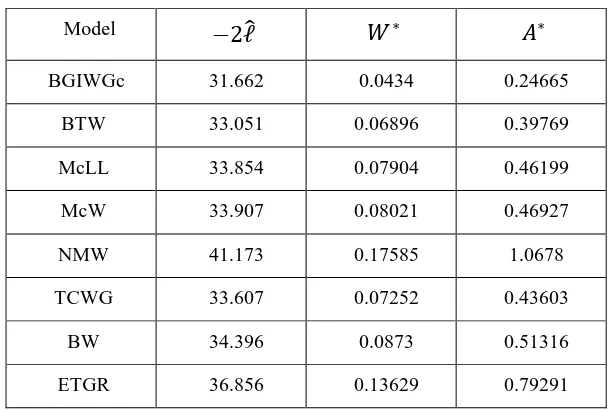
Tables 2 list the values of ̂, and whereas the MLEs of the model parameters and their corresponding standard errors are given in Table 3.
Table 2 compares the fits of the BGIWGc distribution with the BTW, McLL, McW, NMW, TCWG, BW and ETGR distributions. The figures in these tables show that the BGIWGc distribution has the lowest values for ̂, and statistics among all fitted distributions. So, it could be chosen as the best model. The fitted pdf and QQ plot for the BGIWGc distribution are displayed in Figure 3. Figure 4 shows the estimated cdf and sf for the BGIWGc model. It is evident from these plots that the new model provides close fit to the data.
Table 2: Goodness-of-fit statistics for the relief times data
Model ̂
BGIWGc 31.662 0.0434 0.24665
BTW 33.051 0.06896 0.39769
McLL 33.854 0.07904 0.46199
McW 33.907 0.08021 0.46927
NMW 41.173 0.17585 1.0678
TCWG 33.607 0.07252 0.43603
BW 34.396 0.0873 0.51316
Table 3: MLEs and their standard errors for the relief times data
Model Estimates (standard errors)
BGIWGc 19.1874 20.5968 1.4346 9.8485 39.2308 5.8015
( ) (33.03) (43.241) (0.837) (2.001) (63.252) (4.346)
BTW 5.6186 0.5311 53.3438 3.5683 -0.7718
( ) (9.353) (0.148) (111.453) (4.265) (3.894)
McLL 0.8811 2.0703 19.2254 32.0332 1.9263
( ) ( ) ( ) ( ) ( ) ( )
McW 2.7738 0.3802 79.108 17.8976 3.0063
( ) (6.38) (0.188) (119.131) (39.511) (13.968)
NMW 0.1215 2.7837 0.0003 2.7871
( ) ( ) ( ) ( ) ( ) ( )
TCWG 43.6627 5.1271 0.2823 -0.2713
( ) ( ) ( ) ( ) ( )
BW 0.8314 0.6126 29.9468 11.6319
( ) ( ) ( ) ( ) ( )
ETGR 0.1033 0.6917 -0.342 23.5392
( ) ( ) ( ) ( ) ( )
Figure 3: The fitted pdf and QQ plot of the BGIWGc model
6. Conclusions
In this paper, we propose a new six-parameter model called the beta generalized inverse Weibull-geometric (BGIWGc) distribution, which extends the generalized inverse Weibull-geometric (GIWGc) distribution. The BGIWGc density function can be expressed as a linear mixture of GIWGc densities. We derive explicit expressions for some of its mathematical properties. We discuss maximum likelihood estimation. The proposed distribution provides better fits than some other competitive models using a real data set. We hope that the proposed model will attract wider applications in applied areas such as lifetime analysis, hydrology, reliability, engineering.
Appendix A:
The pdfs of the fitted distributions are given (for ) by
BTW: * + ,* + *
, * + * +-
McLL: ( )
* ( ) + . { * ( ) + } /
McW:
* + , * + -
NMW: [ ] ( )
TCWG: * +
* +
ETGR: , [ ] -
[ ] , [ ]
BW: * +
The parameters of the above pdfs are all positive real numbers except for the TCWG and ETGR distributions for which | | .
References
1. Adamidis, K., Dimitrakopoulou, T. and Loukas, S. (2005). On an extension of the exponential-geometric distribution. Statistics & probability letters, 73, 259-269.
2. Adamidis, K. and Loukas, S. (1998). A lifetime distribution with decreasing failure rate. Statistics and Probability Letters, 39, 35-42.
4. Afify, A. Z., Nofal, Z. M. and Ebraheim, A. N. (2015). Exponentiated transmuted generalized Rayleigh distribution: A new four parameter Rayleigh distribution. Pakistan Journal of Statistics and Operations Research, 11, 115-134.
5. Afify A. Z., Yousof, H. M. and Nadarajah, S. (2017). The beta transmuted-H family for lifetime data. Statistics and Its Interface, 10, 505-520.
6. Almalki, S. J. and Yuan, J. (2013). A new modified Weibull distribution. Reliability Engineering and System Safety, 111, 164-170.
7. Barreto-Souza, W., Santos A. H. S., Cordeiro, G. M. (2010). The beta generalized exponential distribution, Journal of Statistical Computation and Simulation, 80, 159-172.
8. Bidram. H (2012). The Beta Exponential-Geometric Distribution. Communications in Statistics- Simulation and Computation, 41, 1606-1622.
9. Cordeiro, G. M., Hashimoto, E. M. and Ortega, E. (2014). The McDonald Weibull model. Statistics, 48, 256-278.
10. Eugene, N., Lee, C., Famoye, F. (2002). Beta-normal distribution and its applications. Communications in Statistics-Theory and Methods, 31, 497-512.
11. de Gusmão, F. R., Ortega, E. M. M. and Cordeiro, G. M. (2011). The generalized inverse Weibull distribution. Statistical Papers, 52, 591-619.
12. Gradshteyn, I. S. and Ryzhik, I. M. (2000). Table of Integrals, Series and Products (sixth edition).San Diego: Academic Press.
13. Gross, A. J. and Clark, V. A. (1975). Survival distributions: Reliability Applications in the Biomedical Sciences. John Wiley and Sons, New York.
14. Khan, M. S. (2010). The beta inverse Weibull distribution. International Transactions in Mathematical Sciences and Computer, 3, 113-119.
15. Keller, A. Z., Goblin, M. T. and Farnworth, N. R. (1985). Reliability analysis of commercial vehicle engines. Reliability Engineering, 10, 15-25.
16. Lee, C., Famoye, F. and Olumolade, O. (2007). Beta-Weibull distribution: Some properties and applications to censored data. Journal of Modern Applied Statistical Methods, 6, 173-186.
17. Mead, M. E., Afify, A. Z., Hamedani, G. G. and Ghosh, I. (2017). The beta exponential Fréchet distribution with applications. Austrian Journal of Statistics, 46, 41-63.
18. Nadarajah, S. and Gupta, A.K. (2004). The beta Fréchet distribution. Far East Journal of Theoretical Statistics,14, 15-24.
19. Nadarajah, S., Kotz, S. (2006). The beta exponential distribution. Reliability Engineering and System Safety, 91, 689-697.