Correspondence:Haruo Sato ([email protected]) Received: 10 October 2018 – Discussion started: 25 October 2018
Revised: 14 December 2018 – Accepted: 10 January 2019 – Published: 5 February 2019
Abstract.Recent seismological observations focusing on the collapse of an impulsive wavelet revealed the existence of small-scale random heterogeneities in the earth medium. The radiative transfer theory (RTT) is often used for the study of the propagation and scattering of wavelet intensities, the mean square amplitude envelopes through random media. For the statistical characterization of the power spectral den-sity function (PSDF) of the random fractional fluctuation of velocity inhomogeneities in a 3-D space, we use an isotropic von Kármán-type function characterized by three parame-ters: the root mean square (RMS) fractional velocity fluctu-ation, the characteristic length, and the order of the modi-fied Bessel function of the second kind, which leads to the power-law decay of the PSDF at wavenumbers higher than the corner. We compile reported statistical parameters of the lithosphere and the mantle based on various types of mea-surements for a wide range of wavenumbers: photo-scan data of rock samples; acoustic well-log data; and envelope analy-ses of cross-hole experiment seismograms, regional seismo-grams, and teleseismic waves based on the RTT. Reported ex-ponents of wavenumber are distributed between−3 and−4, where many of them are close to −3. Reported RMS frac-tional fluctuations are on the order of 0.01–0.1 in the crust and the upper mantle. Reported characteristic lengths dis-tribute very widely; however, each one seems to be restricted by the dimension of the measurement system or the sample length. In order to grasp the spectral characteristics, elimi-nating strong heterogeneity data and the lower mantle data, we have plotted all the reported PSDFs of the crust and the upper mantle against wavenumber for a wide range (10−3– 108km−1). We find that the spectral envelope of those PSDFs
is well approximated by the inverse cube of wavenumber. It suggests that the earth-medium randomness has a broad spec-trum. In theory, we need to re-examine the applicable range
of the Born approximation in the RTT when the wavenumber of a wavelet is much higher than the corner. In observation, we will have to carefully measure the PSDF on both sides of the corner. We may consider the obtained power-law decay spectral envelope as a reference for studying the regional dif-ferences. It is interesting to study what kinds of geophysical processes created the observed power-law spectral envelope at different scales and in different geological environments in the solid earth medium.
1 Introduction
The first image of the solid earth is composed of spheri-cal shells, for example, PREM (preliminary reference Earth model) (Dziewonski and Anderson, 1981). As seismic net-works were deployed on the regional scale and worldwide, the velocity tomography based on the ray tracing method re-vealed 3-D heterogeneous structures at various scales; how-ever, spatial variations in the resultant velocity structure are essentially smooth compared with seismic wavelengths. Aki and Chouet (1975) first put a focus on long-lasting coda waves of small earthquakes and interpreted them as scat-tered waves by small-scale random heterogeneities. They proposed to measure the scattering coefficient g, the scat-tering power per unit volume as a measure of medium het-erogeneity. They analyzed the mean square (MS) amplitude time trace of coda waves as an incoherent sum of scattered wave power by using the Born approximation (e.g., Chernov, 1960), which is a simplified version of the radiative transfer theory (RTT). There have been many measurements of the total scattering coefficientgisosupposing isotropic scattering
on the order of 10−2km−1for 1–20 Hz in the lithosphere, and it marks a higher value beneath active volcanoes (e.g., Sato et al., 2012; Yoshimoto and Jin, 2008). There were pre-cise measurements of regional variations in giso as Carcolé
and Sato (2010) in Japan and Eulenfeld and Wegler (2017) in the US. Hock et al. (2004) analyzed medium heterogeneity in Europe from the analyses of teleseismic waves using the modified energy flux model (Korn, 1993). There were also measurements of the anisotropic scattering coefficient from the analysis ofScoda envelopes (e.g., Jing et al., 2014; Zeng, 2017).
Aki and Chouet (1975) derived the angular dependence of the scattering coefficient of scalar waves from the power spectral density function (PSDF) of the fractional velocity fluctuation using the Born approximation. Sato (1984) ex-tended the envelope synthesis of scalar waves to the whole envelope synthesis of three-component seismograms from theP onset toScoda on the bases of the single scattering ap-proximation of the RTT. His syntheses explain how seismo-gram envelopes in different back azimuths vary depending on the source fault mechanism. Extension to the multiple scat-tering case was developed by using Stokes parameters (e.g., Margerin et al., 2000; Margerin, 2005; Przybilla et al., 2009; Sanborn et al., 2017). We also note that Monte Carlo sim-ulation was developed to stochastically solve the RTT (e.g., Hoshiba et al., 1991; Gusev and Abubakirov, 1987; Yoshi-moto, 2000). For the data processing, it is more appropriate to stack MS envelopes of observed seismograms for com-parison with the averaged intensity time traces stochastically synthesized by the RTT (e.g., Shearer and Earle, 2004; Rost et al., 2006; da Silva et al., 2018).
When the central wavenumber of a wavelet increases much larger than the corner wavenumber of the PSDF, the wavelet around the peak value is mostly composed of narrow-angle scattering around the forward direction. In such a case, the Born approximation becomes inappropriate; how-ever, the phase shift modulation based on the parabolic proximation is useful, which is called the phase screen ap-proximation. As an extension of the RTT with the phase screen approximation, the Markov approximation was also used for the analysis of envelope broadening and peak de-lay with increasing travel distance (e.g., Sato, 1989; Saito et al., 2002; Takahashi et al., 2009). Kubanza et al. (2007) measured regional differences in the lithospheric heterogene-ity from the partitioning of seismic energy of teleseismicP waves into the vertical and transverse components based on the Markov approximation.
There have been various kinds of measurements of the PSDF of the random velocity fluctuation, where the PSDF is often supposed to be a von Kármán type. In the following section, the main objective is to compile reported PSDF mea-surements in various scales in different geological environ-ments of the solid earth: photo scanning of small rock sam-ples, acoustic well logs, array analyses of teleseismic waves, waveform analyses using finite difference (FD) simulations,
and analyses of seismogram envelopes on the basis of the RTT. We enumerate their statistical parameters and plot their PSDFs against wavenumber. We will show that the envelope of all the PSDFs is well approximated by a power-law decay curve. Then, we will discuss the results obtained and a few problems in the envelope synthesis theory for such random media and the geophysical origin of such power spectra.
2 Statistical characterization of random media
We consider the propagation of scalar waves as a sim-ple model, where the inhomogeneous velocity is given by V (x)=V0(1+ξ(x)). The fractional fluctuationξ(x)is
sup-posed to be a random function of space. We imagine an en-semble of random media{ξ(x)}, wherehξ(x)i =0. Angular brackets mean the ensemble average. We suppose that ran-dom media are homogeneous and isotropic, then we statisti-cally characterize them by using the autocorrelation function (ACF):
R(x)=R(r)= hξ(y)ξ(y+x)i, (1a)
wherer= |x|. The MS fractional fluctuation as a measure of the strength of randomness is supposed to be small, andε2≡ R(0)1. The Fourier transform of ACF gives the PSDF:
P (m)=P (m)= ∞ Z Z Z
−∞
R(x)e−imxdx, (1b)
where wavenumberm= |m|. In some literature,(2π )−3 is used as a prefactor in the right-hand side of Eq. (1b). 2.1 Several types of random media
There are several types of PSDF and ACF characterized by a few parameters.
2.1.1 von Kármán type
The ACF is written by using a modified Bessel function of the second kind of orderκand characteristic lengtha:
R(r)=2
1−κ
0(κ)ε
2r
a κ
Kκ r
a
forκ >0, (2a)
which is an exponential typeR(r)=ε2e−r/awhenκ=1/2. In the case of space dimensiond, the PSDF is
P (m)= 2
dπd20(κ+d
2)ε
2ad
0(κ) 1+a2m2κ+d2
forκ >0
∝m−2κ−dforma−1. (2b)
Figure 1. (a)Log–log plot of PSDF vs. wavenumbermin 3-D space (von Kármán type,κ=0.1, 0.5, and 1; Henyey–Greenstein type, HG,
κ=0; Gaussian type, G).(b)Linear plot of ACF vs. lag distancer.
the 1-D case, where κ corresponds to the Hurst number. In the following, we will basically use a von Kármán-type func-tion for characterizing the earth-medium heterogeneity.
Especially for an anisotropic case, we define the von Kármán-type PSDF in 3-D (e.g., Wu et al., 1994; Nakata and Beroza, 2015):
P (m)= 2
3π320(κ+3
2)ε2axayaz 0(κ)
1+a2
xm2x+ay2m2y+az2m2z
κ+32
forκ >0. (3)
2.1.2 Henyey–Greenstein type
For a case formally corresponding to κ=0 of the von Kármán-type PSDF, we define the Henyey–Greenstein type ACF and PSDF in 3-D (Henyey and Greenstein, 1941): R(r)=ε2K0
r a
, (4a)
P (m)= 2π
2ε2a3
(1+a2m2)3/2 ≈2π
2ε2m−3forma−1. (4b)
Note that parameterε2characterizesP butε26=R(0)since R(r)diverges asr→0.
2.1.3 Gaussian type
Gaussian-type ACF and PSDF are also used because they are mathematically tractable.
R(r)=ε2e− r2
a2, (5a)
P (m)=pπ3ε2a3e−m2a2
4 . (5b)
We plot those PSDFs against wavenumber and ACFs against lag distance in Fig. 1.
3 Measurements of random heterogeneities
plot-ting PSDFs in the figures. Measurement with a label with an asterisk∗is insufficient for plotting the PSDF in the figures.
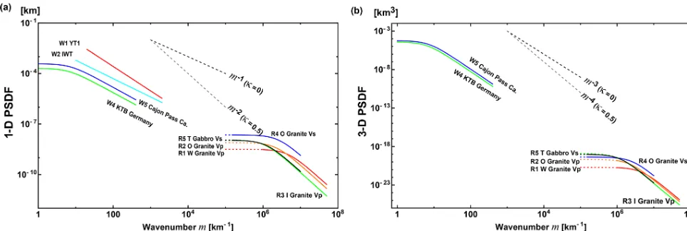
3.1 Photo scan of the rock surface
The photo-scan method uses a scanner to take a picture of the polished flat surface of a small rock sample (e.g., Sivaji et al., 2002; Spetzler et al., 2002; Fukushima et al., 2003). For the case of a granite sample, those papers classified color images on a straight line into three types of mineral grains: quartz, plagioclase, and biotite. Assigning a typical velocity VP orVS to each mineral grain, they constructed a velocity
profile along the line. Then, they estimated the 1-D PSDF of the velocity fractional fluctuation. They measured 1-D PS-DFs of granite and gabbro samples fixingκ=0.5 as R1–R5. Figure 2a shows estimated 1-D PSDFs, where the wavenum-ber range is on the order of 1 mm−1. We note that raw 1-D
PSDFs in Figs. 4 and 5 of Fukushima et al. (2003) decay a little slower than those of R4 and R5 in Fig. 2a, especially at large wavenumbers.
3.1.1 Conversion from 1-D PSDF into 3-D PSDF In the case of isotropic randomness, we evaluate the 1-D PSDF from the 3-D ACF along the zaxis at x=y=0 as follows:
P1−D(mz)≡ ∞ Z
−∞
R3-D(0,0, z) e−imzzdz
= ∞ Z −∞ 1
(2π )3
∞
Z Z Z
−∞
P3-D
m0x, m0y, m0z
eim0zzdm0
e−imzzdz
= 1
(2π )2 ∞ Z Z
−∞ P3-D
m0x, m0y, mz
dm0xdm0y. (6a)
Substituting Eq. (2b) into the above equation, we have P1−D(mz)
= 1
(2π )2 ∞ Z Z
−∞
8π3/2ε2a30 (κ+3/2) 0 (κ)
h
1+a2m0
x2+m0y2+m2z
iκ+3/2dm 0 xdm
0 y
= 2π
1/20 (κ+1/2) ε2a
0 (κ) 1+a2m2 z
κ+1/2. (6b)
Thus, we can evaluate the 3-D PSDF from the 1-D PSDF using parametersε,κ, andaof 1-D PSDF.
Supposing the randomness is isotropic, we evaluate corre-sponding 3-D PSDFs of R1–R5 and plot them in Fig. 2b. 3.2 Acoustic well logs in boreholes
An acoustic well log is obtained from the measurement of the travel time of an ultrasonic pulse along the wall of a
Figure 2. (a)1-D PSDF vs. wavenumber for rock samples and acoustic well logs.(b)Converted 3-D PSDF vs. wavenumber, where the randomness is supposed to be isotropic. See labels in Table 1.
borehole. Measurements W1 (volcanic tuff) and W2 (tertiary to pre-tertiary) in Japan clearly show power-law decay with κ=0.225 and 0.045, respectively; however, a corner is not clearly seen in each PSDF. Measurement W4 at the deep well KTB in Germany shows κ=0.10. Measurement W3 in the same well shows that the exponent of wavenumber is −0.97, which formally corresponds to a negative κ. Mea-surement W5 at Cajon Pass in California shows κ=0.11. All these measurements show very smallκ values close to 0. Shiomi et al. (1997) made a list of reported exponents of wavenumber, which shows that most κ values are smaller than 0.25. Measurement of a seems to be restricted by the sample length. We enumerate those measurements in Table 1 and plot their 1-D PSDFs against wavenumber in Fig. 2a. Figure 2b plots the corresponding 3-D PSDFs of W4 and W5. We note that Wu et al. (1994) measured anisotropy of ran-domness from the analysis of well logs obtained from two parallel wells at KTB: the ratio of characteristic scales in horizontal to vertical directions ah/az=1.8 (see Eq. 3) as
shown in W3.
3.3 Velocity tomography
There have been measurements of velocity tomography at various scales, from which we can calculate the PSDF and then estimate von Kármán-type parameters. This method de-pends on the spatial resolution of the tomography result. Measurement L1 in Table 2 is calculated from the preciseVP
tomography result of the shallow crust, Los Angeles, Cal-ifornia: the exponent of wavenumber is −3.08 (κ=0.04). Anisotropic randomness is also reported:az=0.1 andah=
0.5 km (see Eq. 3), we show those in Fig. 3a. Measurement M2 in Table 3 is evaluated from the 2-D PSDF of theVS
to-mography result of the upper mantle in a low wavenumber range. Although there is a resolution limit of the tomography method, the exponent of wavenumber is between−2 and−3,
which means 0< κ <0.5. We note that Fig. 8 of Mancinelli et al. (2016a) shows that the 1-D PSDF estimated from the VP tomography result in the upper mantle (Meschede and
Romanowicz, 2015) covers that of MU2 (κ=0.05,ε=0.1, a=2000 km) for the wavenumber range from 2×10⁻⁴to 10−2km−1.
3.4 Array analysis of teleseismicP waves
Teleseismic P waves registered by a large aperture array were used for the evaluation of the 3-D PSDF of the litho-sphere beneath the array: LA1 and LA2 of Table 2 in Mon-tana and LA3 in southern California used amplitude and phase coherence analyses, where a Gaussian-type PSDF (Eq. 5b) was assumed because of mathematical simplicity. As shown in Fig. 3b, they drop very fast as wavenumber in-creases. Later Flatté and Wu (1988) developed the angular coherence analysis in addition to the above methods. Ana-lyzing teleseismicP waves registered at NORSAR, they pro-posed an overlapping two-layer model LA4, which is com-posed of a band-limited flat spectrum from the surface to 200 km of depth andm−4spectrum (κ=0.5,ε=0.01–0.04) for depths from 15 to 250 km. It meansκ <0.5 and the decay of their PSDF is much smaller than that of Gaussian types (not shown in Fig. 3b).
3.5 Finite difference (FD) simulations
Figure 3.3-D PSDF vs. wavenumber for(a)the lithosphere (the crust and uppermost mantle),(b)strong heterogeneities and array data analyses in the lithosphere. See labels in Table 2.
Figure 4.3-D PSDF vs. wavenumber for the upper and lower mantle. See labels in Table 3.
subducting oceanic plate is an efficient waveguide for high-frequency seismic waves: estimated anisotropic parameters are κ=0.5 and ε=0.02 withap=10 km and at=0.5 km
in the parallel and transverse directions, respectively. Note that ML2 supposes a Gaussian-type function.
3.6 Analyses of seismogram intensities (MS amplitude envelopes)
The RTT is essentially stochastic to directly synthesize the intensity (the average MS amplitude envelope) of a wavelet propagating through random media. There are two conven-tional methods on the basis of the RTT: one uses the Born
approximation and the other uses the phase screen approx-imation based on the parabolic approxapprox-imation when the wavenumber is larger than the corner. The former neglects the phase shift, but the latter correctly considers the phase shift.
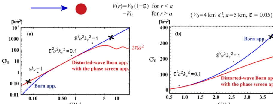
3.6.1 Scalar wave scattering by a single obstacle We here study the deterministic scattering of scalar waves by a single spherical obstacle (radiusa=5 km and velocity anomalyε= +0.05) embedded in a homogeneous medium (V0=4 km s−1) as a mathematical model. The Born
Figure 5.3-D PSDF vs. wavenumber for all the data.
putting the incident plane wave of wavenumberkcin the
in-teraction term of the first-order perturbation equation. From the scattering amplitude we evaluate the total scattering cross section σ0 as a measure of scattering power of the
obsta-cle. The resultantσ0monotonously increases with frequency
as shown by a blue line in Fig. 6. As the wavenumber increases (akc1), the phase shift increases as the
inci-dence plane wave penetrates into the obstacle. Putting the phase modulated wave according to the parabolic approxi-mation (the phase screen approxiapproxi-mation) into the interaction term of the first-order perturbation equation, we calculate the scattering amplitude and then the total scattering cross sec-tion. This is the distorted-wave Born approximation with the phase screen approximation, which is also referred to as the eikonal approximation. This approximation predicts thatσ0
(a red line in Fig. 6) saturates at high frequencies and con-verges to 2π a2, which is twice the geometrical section area of the obstacle as predicted by shadow scattering (e.g., Lan-dau and Lifshitz, 2003, p. 519 and 543). We recognize that the conventional Born approximation is still accurate even forakc>1; however, it works well only forε2a2kc2.O(0.1).
We should use the distorted-wave Born approximation with the phase screen approximation forε2a2kc2&O(1). The two approximations predict nearly the same σ0 value in the
in-termediate range. We note that 2εakc is the phase shift on
the center line after passing the obstacle. Note that the phase screen approximation is not applicable forakc<1 since it is
based on the parabolic approximation.
Interpreting ε and a as the RMS fractional fluctuation and the characteristic length of uniformly distributed ran-dom media, we may use the inequality ε2a2k2cO(1)or
ε2a2k2c.O(0.1) as a criterion of the Born approximation used in the RTT.
3.6.2 RTT with the Born approximation
For uniformly distributed random media characterized by P (m), the Born approximation leads to the scattering coeffi-cient at wavenumberkcinto scattering angleψ:
g(kc, ψ )=
kc4
πP (2kcsin ψ
2), (7a)
which is axially symmetric. The total scattering coefficient is
g0(kc)≡
1 4π
I
g(kc, ψ )d=
1 2
π Z
0
g(kc, ψ )sinψdψ
=
2kc
Z
0
gker(kc, m)dm, (7b)
wherem=2kcsinψ2. The integral kernel in the wavenumber
space is given by
gker(kc, m)=
k2c
2πmP (m). (7c)
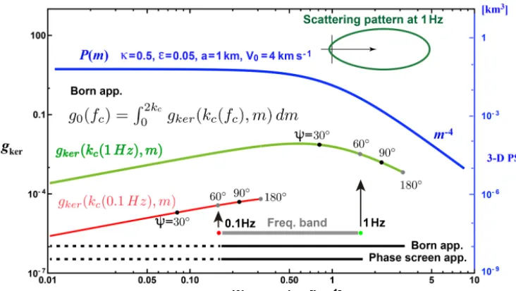
The upper bound of the integral is twice the wavenumber. As an example, Fig. 7 shows plots of P (m) (blue) vs. m, andgker(m)vs.mat 0.1 Hz (red) and 1 Hz (green) for the
case ofκ=0.5,ε=0.05,a=1 km, andV0=4 km s−1. As
Figure 6.Deterministic scattering of scalar waves by a high-velocity sphere.(a)Log–log plot of the total scattering cross section against frequency.(b)Semi-log plot for zoomed in graph. The Born approximation and the distorted-wave Born approximation with the phase screen approximation are drawn by blue and red lines, respectively.
(green) has a large lobe into the forward direction; however, it becomes isotropic as the frequency decreases. Dots on each gkercurve show corresponding scattering angles.
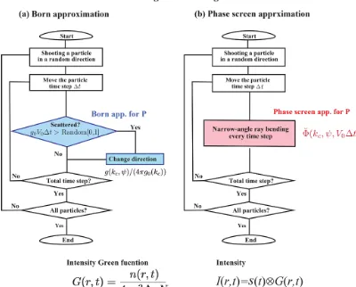
In the framework of the RTT, the Monte Carlo simulation is a simple method to stochastically synthesize the wavelet intensity time trace. A particle carrying unit intensity is shot randomly from a point source, and its trajectory is traced with the increment of time steps. The occurrence of scatter-ing is stochastically tested by the inequalityg0V01t >
Ran-dom[0,1] at every time step of1t, andg(kc, ψ )/(4π g0(kc))
is used as the probability of scattering into angle ψ. Note that Random[0,1] is a uniform random variable between 0 and 1. Sinceg0V01tis chosen to be small enough, scattering
does not occur every time step but intermittently. As a sim-ple examsim-ple, Fig. 8a schematically illustrates the flowchart of the Monte Carlo simulation for the isotropic radiation from a point source in uniform random media. At lapse timet, divid-ing the number of particlesnregistered in a spherical shell of radiusrand a thickness1rby the total number of particles N and the shell volume 4π r21r, we calculate the intensity Green functionG(r, t ). The intensity time traceI (r, t )is cal-culated by the convolution ofG(r, t )and the source intensity time functionS(t )in the time domain. It is easy to introduce a layered structure of background velocity and intrinsic ab-sorption into the simulation code.
The RTT for the scalar wave case can be extended to the elastic vector wave case by using Stokes parameters. There are four scattering modes: PP, PS, SS, and SP scatterings, and theS-wave scattering coefficients are not axially symmetric (see Sato et al., 2012, Fig. 4.7). Many papers (e.g., Shearer and Earle, 2004; Przybilla et al., 2009) suppose proportional relationsδVp/VP0=δVS/VS0=ξ andδρ/ρ0=ν ξbased on
the empirical Birch’s law, which reduce three fractional fluc-tuations into one (e.g., Sato et al., 2012, Eqs. 4.58 and 4.59). The RTT with the Born approximation has been often used not only for the analyses ofScoda envelopes but also for the whole seismogram envelope from theP onset via P coda throughS wave until S coda (see Tables 2 and 3). This method has been often used not only for the analyses of regional seismograms propagating through the lithosphere but also for the analyses of teleseismic waves propagating through the mantle. This method is not only applied to direct P phase waves but also PcP and PKPprec phase waves and
so on. In this review, we neglect intrinsic attenuation param-eters a priori assumed or measured in each paper. For a given wavenumber range(kl, ku)(gray) in Fig. 7, each PSDF curve
using this method in Figs. 3–5 and 9 is drawn by a dotted line for(0, kl)and a solid line for(kl,2ku)as the line next to the
bottom of Fig. 7. As indicated by dots on thegker curves,
the wavenumber interval of the solid line reflects wide-angle scattering and that of dotted line reflects narrow-angle scat-tering around the forward direction.
Figure 7.Plot ofP (m)(blue, right scale) and the spectral kernel of the scattering coefficientgker(kc(fc), m)atfc=0.1 Hz (red, left scale)
and 1 Hz (green, left scale) according to the Born approximation. Scattering angles are marked by dots on each trace. For the case of the frequency band between 0.1 and 1 Hz, the phase screen approximation based on the parabolic approximation covers the wavenumber range from 0 to the upper bound (line at the bottom); however, the Born approximation covers the range from 0 to twice the upper bound (line next to the bottom). We also use these line styles in Figs. 3–5 and 9.
proposed an alternative model of 3-D PSDF∝m−2.6in ad-dition to ML3 (not shown in Fig. 4).
3.6.3 RTT with the phase screen approximation
Whenakc1, scattering mostly occurs within a narrow
an-gle around the forward direction. At a large travel distance, the wavelet just after the onset is mostly composed of those waves. The phase screen approximation correctly calculates the phase shift modulation. For the incidence of a plane wave into thezdirection, the mutual coherence function (MCF) of the phase shift modulated waves for an increment1zis given by
8(kc, r⊥, 1z)=e−k 2
c(A(0)−A(r⊥))1z. (8a)
The longitudinal integral of the ACF is
A(r⊥)= ∞ Z
−∞
R(x⊥, z)dz
= 1
(2π )2 ∞ Z Z
−∞
P (m⊥, mz=0)eim⊥x⊥dm⊥, (8b)
wherex⊥is the transverse coordinate vector andr⊥= |x⊥|
(Sato et al., 2012, Eq. 9.60). Taking the Fourier transform of
MCF8with respect to transverse coordinates, we have
˘
8(kc, k⊥, 1z)=
1 (2π )2
∞ Z Z
−∞
8(kc, r⊥, 1z)eik⊥x⊥dx⊥
−→
1z→0δ(k⊥). (8c)
Since RR∞−∞8(k˘ c, k⊥, 1z)dk⊥=1, interpreting ˘
8(kc, k⊥, 1z) as the probability of ray-bending angle ψ=tan−1k⊥
Figure 8.Flowchart of the Monte Carlo simulation code according to the RTT for the scalar wavelet intensity in uniform random media.
(a)RTT with the Born approximation.(b)RTT with the phase screen approximation.
When this approximation is used,kca−1is a priori
sup-posed. Most of this type of measurement reads the peak de-lay and the envelope width of each seismogram envelope. There is some merit to the fact that the peak delay mea-surement is rather insensitive to intrinsic absorption. In NE Japan, aκvalue beneath a volcano LS2 is smaller than those in the fore-arc side L12 and L13. Note that narrow-angle scattering around the forward direction dominates in teleseis-mic wavelets even if the Born approximation is used for the analysis. Narrow-angle scattering is mostly produced by the PSDF in low wavenumbers compared with kc. For a given
wavenumber range(kl, ku)(gray) in Fig. 7, each PSDF curve
using this method in Fig. 3 is drawn by a dotted line for(0, kl)
and a solid line for(kl, ku)as the bottom line of Fig. 7.
3.7 Characteristics of reported PSDFs 3.7.1 All the data
Some measurements a priori assumed κ=0.5; however, most of measurements reportκ <0.5. In the mantle,κis very small and close to zero, and a HG-type function is also
pro-posed. The RMS fractional fluctuationε is on the order of 0.1 for rock samples and well-log data, and in the range from 0.01 to 0.1 in the lithosphere and the upper mantle. Large val-ues are reported for the shallow crust L16 and beneath a vol-cano LS3; however, smaller values are reported for the lower mantle. The characteristic scalea varies a lot depending on measurements. The corner wavenumbera−1 is not clearly seen in PSDFs of acoustic well logs. Some measurements re-port anisotropy: W3 of well-logs, L1 of velocity tomography in the shallow crust, and LS5 in the subducting oceanic slab. The characteristic length in the vertical direction is smaller than the horizontal direction in the shallow crust, and that in the transverse direction is smaller than that in the direction parallel to the subducting slab.
val-Figure 9.3-D PSDF vs. wavenumber for the crust and the upper mantle. Data of Gaussian-type, anisotropy type, strong heterogeneity, the lower mantle, and the whole mantle are excluded. The light-gray straight line visually fits to most spectral envelopes.
ues, and those for volcanoes and for the shallow crust take larger values than others.
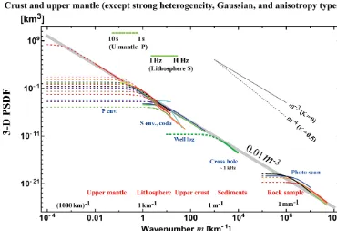
3.7.2 Lithosphere and the upper mantle except strong heterogeneity, Gaussian, and anisotropy types Eliminating data supposing a Gaussian-type data LA1–LA3, strong heterogeneity data LS1–LS4, anisotropy-type data L1 and LS5, and the lower mantle and the whole mantle data ML1–ML4 and MW1–MW2 from Fig. 5, we plot the rest of the data for the crust and the upper mantle in Fig. 9. Most εvalues are in the range of 0.01–0.1, mostκ values are less than or equal to 0.5 and many of them are close to 0, and the high wavenumber end of the power-law decay branch of each PSDF is not far from each corner wavenumber.
We draw a power-law decay line PSDF(m)= 0.01m−3km3(gray) visually fitting to most PSDF envelopes for a very wide range of wavenumbers (10−3–108km−1). This line is not the average of PSDFs. This line looks like an extension of MU2 in the upper mantle into higher wavenumbers of the shallow crust.
4 Discussions 4.1 Measurements
It will be necessary for us to measure the small-scale ran-domness of sedimentary rock samples. More measurements
are necessary in the wavenumber range 103–105km−1since there are few measurements.
In most PSDF measurements, each power-law decay branch is short since the Born approximation senses the spectrum up to twice the wavenumber. It will be necessary to measure how each power-law decay branch varies with wavenumber increasing. It will be necessary to estimate the cornera−1 in each measurement with a wide wavenumber range covering, sufficiently large enough, both sides of the corner. The flat part, the low-wavenumber side of each PSDF drawn by a dotted line in figures is also important as the cause of narrow-angle scattering.
Although most measurements used in this review analyzed intrinsic attenuation, we did not enumerate them in this re-view since different assumptions were used in different surements. It will be necessary for us to systematically mea-sure the PSDF of random heterogeneity in conjunction with intrinsic attenuation.
We should note that there are large variations in δlnVS/δlnVPandν≡δlnρ/δlnVSin the earth. Koper et al.
(1999) estimatedδlnVS/δlnVPto be in the range 1.1–1.5 in
the Tonga Slab. Romanowicz (2001) estimatedδlnVS/δlnVP
T able 3. Reported v on Ka ´rmán parameters of the upper mantle and the lo wer mantle. A v alue in parentheses ( ) is a priori assumed in gi v en by a range, a v alue in square brack ets [ ] is used for plotting the PSDF . A label with an asterisk ∗is insuf ficient for plotting the PSDF Label Re gion Data & method 3-D PSDF (km 3) κ ε a (km) f range (Hz) Upper mantle MU1 ∗ U. mantle Vs T omograph y, 2-D ∝ m − 2 to − 3km 2 0–0.5 – > 500 – MU2 U. mantle T ele. P en v., SEM, Born – 0.05 0.1 2000 0.017–0.2 MU3 U. mantle T ele. P en v., Born – (0.5) 0.03–0.04 [0.035] 4 0.5–2 Lo wer mantle ML1 L. mantle T ele. P en v., Born – (0.5) 0.005 8 0.5–2 ML2 M. L. mantle PKIKP prec., FD – (Gaussian) 0.01 20 0.02–2 ML3 M. L. mantle PKP prec., Born 2 . 5 × 10 − 5m − 3 0, HG 0.002 15 [30] 0.5–4 ML4 M. L. mantle PcP en v., Born, FD – (0.5) 0.002–0.01[0.005] 8 0.8–1.5 Whole mantle MW1 Whole mantle PKP prec., Born 1 . 4 × 10 − 5m − 3 0, HG 0.001–0.002 [0.0015] 8 [30] 0.4–2.5 MW2 Whole mantle PP prec., Born – (0.5) 0.008–0.01 [0.009] 8 0.5–2.5
In Sect. 3.6.1, we mentioned that the conventional Born ap-proximation is inapplicable and the phase screen approxi-mation is useful when the phase shift becomes large as the wavenumber increases. In order to avoid the difficulty, taking the center wavenumber of a wavelet as a reference, Sato and Emoto (2018) proposed to divided the PSDF into two com-ponents (see also Sato, 2016; Sato and Emoto, 2017). They use the Born and phase-screen approximations to the short-scale (high wavenumber) and long-short-scale (low wavenumber) components,PS andPL, respectively, in the RTT in order
to simultaneously explain the envelope broadening just after the onset and the excitation of late coda waves. Figure 10 illustrates the flowchart of their Monte Carlo simulation. Their spectrum division method looks like an implementa-tion of the distorted-wave Born approximaimplementa-tion in the RTT since it describes wide-angle scattering for the incidence of the phase-shift modulated wave. They successfully synthe-sized intensity time traces that explain FD simulation results for the case ofakc=23.6 andε2a2k2c=1.39. It would be
interesting to see how this method may be extended to polar-ized elastic waves.
We note that some papers numerically show that the RTT with the Born approximation works well in some cases over the above limitation. Przybilla et al. (2006) synthesizes vector-wave intensity that fits to that of the FD simulation in 2-D, even forSwaves ofakc=58 andε2a2k2c=8.4 (see
their Table 1) if the wandering effect is convolved as a re-sult of the travel time fluctuation. Emoto and Sato (2018) show that the synthesized scalar intensity by the RTT with the Born approximation fits to that of the FD simulation in 3-D, even for the case ofakc=23.6 andε2a2k2c=1.39 when
the wandering effect is convolved. If the earth heterogene-ity is represented by a power-law decay power spectrum for such a wide wavenumber range, which means that the corner wavenumber is very low, we should carefully examine the applicability of the Born approximation in the RTT.
seis-Figure 10.Spectrum division method.(a)Division ofP into two components,PSandPL, with respect to the center wavenumber of a wavelet
kcas a reference, whereζis a tuning parameter.(b)Flowchart of the Monte Carlo simulation according to the RTT with the spectrum division
method. Modified from Sato and Emoto (2018).
mograms do not only reflect those but also the scattering contribution of pores and cracks distributed over the earth medium. It will be necessary for us to study their contribu-tion in the intensity synthesis.
4.3 Power-law decay spectral envelope
In observation, we may take the power-law spectral envelope as a reference curve for studying the regional differences, especially in the power-law decay part of the PSDF. The characteristic length a seems to increase as the wavenum-ber of a wavelet decreases or as the dimension of measure-ment system becomes large. It reminds us that the character-istic scale of the slip distribution increases with increasing source dimension as Mai and Beroza (2002) analyzed finite-fault source inversion results (see their Fig. 12).
The power-law decay spectral envelope reminds us of the observed fractal nature of various kinds of surface topogra-phies: Sayles and Thomas (1978a, b) show a 1-D PSDF ∝m−2 for wavelengths 10−6–103km although the power exponent varies from −1.07 to −3.03 for small segments; Brown and Scholz (1985) show a 1-D PSDF∝m−1.64 to−3.36 for the wavenumber range 10−6to 0.1 µm−1, especially for the topography of natural rock surfaces and faults. We also
note that the PSDF of the refractive index fluctuation of air obeys the Kolmogorov spectrum: 3-D PSDF∝m−11/3, whereκ=1/3. This spectrum is physically produced by the cascade in the turbulent flow of low viscosity air: the large eddies breaks up originating smaller eddies dissipating en-ergy by viscosity. However, it may be difficult to apply this cascade model to the mantle since the viscosity of mantle fluid is thought to be high.
es-and the multiple lapse-time window analysis (Fehler et al., 1992; Hoshiba, 1993) has often been used for practical anal-yses. This method essentially estimatesgisofrom the ratio of
late coda excitation to the radiated energy irrespective of the envelope broadening. Recent measurements show that giso
decreases with depth (e.g., Rachman and Chung, 2016; Badi et al., 2009). It will be interesting to plot the frequency de-pendence of reportedgisofor a wide range of frequencies and
to study the relation with the obtained power spectral enve-lope shown in Fig. 9.
5 Conclusions
Recent seismological observations focusing on the collapse of an impulsive wavelet revealed the existence of small-scale random heterogeneities in the earth medium. The RTT has often been used for the study of the propagation of wavelet intensities, the MS amplitude envelopes. For the statistical characterization of the PSDF of random velocity inhomo-geneities in a 3-D space, we have used von Kármán type functions with three parameters: the RMS fractional veloc-ity fluctuation ε, the characteristic length a, and the order κ of the modified Bessel function of the second kind. This model leads to the power-law decay of PSDF ∝m−2κ−3at wavenumbermhigher than the corner ata−1. We have com-piled reported statistical parameters of the lithosphere and the mantle based on various types of measurements for a wide range of wavenumbers: photo-scan data of rock samples, acoustic well-log data, and envelope analyses of cross-hole experiment seismograms, regional seismograms, and tele-seismic waves based on the RTT. Reportedκvalues are dis-tributed between 0 and 0.5 (PSDF∝m−3 to−4), where many of them are close to 0 (PSDF∝m−3). Reportedεvalues are on the order of 0.01–0.1 in the crust and the upper mantle, where smaller values in the lower mantle and higher values beneath volcanoes. Reportedavalues distribute very widely; however, each one seems to be restricted by the dimension of the measurement system or the sample length. In order to grasp the spectral characteristics, eliminating strong hetero-geneity data and the lower mantle data, we have plotted all
esting to study what kinds of geophysical processes created the power-law spectral envelope at different scales and in dif-ferent geological environments of the solid earth medium.
Data availability. All the data for this review work are listed in Ta-bles 1–3, where all the references are given.
Author contributions. The author HS reviewed reported measure-ment of statistical parameters characterizing the random hetero-geneities in the earth.
Competing interests. The author declares that they have no conflict of interest.
Acknowledgements. This paper is a part of the Beno Gutenberg medal lecture at the 2018 EGU assembly held in Vienna. The author is grateful to the seismology section of EGU for giving him an opportunity for reviewing measurements of random heterogeneities in the solid earth and various theoretical approaches. The author expresses sincere thanks to his colleagues and ex-graduate students who enthusiastically collaborated with him in studying seismic wave scattering in random media. The author acknowledges reviewers, Vernon Cormier, Michael Korn, and Ludovic Margerin and editor Tarje Nissen-Meyer for their helpful comments and suggestions.
Edited by: Tarje Nissen-Meyer
Reviewed by: Ludovic Margerin, Michael Korn, and Vernon Cormier
References
Aki, K.: Scattering of P waves under the Mon-tana LASA, J. Geophys. Res., 78, 1334–1346, https://doi.org/10.1029/JB078i008p01334, 1973.
Allègre, C. J. and Turcotte, D. L.: Implications of a two-component marble-cake mantle, Nature, 323, 123–127, 1986.
Badi, G., Pezzo, E. D., Ibanez, J. M., Bianco, F., Sabbione, N., and Araujo, M.: Depth dependent seismic scattering attenuation in the Nuevo Cuyo region (southern central Andes), Geophys. Res. Lett., 36, L24307, https://doi.org/10.1029/2009GL041081, 2009. Bentham, H., Rost, S., and Thorne, M.: Fine-scale structure of the mid-mantle characterised by global stacks of PP precursors, Earth Planet. Sci. Lett., 472, 164–173, 2017.
Brown, S. R. and Scholz, C. H.: Broad bandwidth study of the to-pography of natural rock surfaces, J. Geophys. Res.-Sol. Ea., 90, 12575–12582, 1985.
Calvet, M. and Margerin, L.: Lapse-Time Dependence of Coda Q: Anisotropic Multiple-Scattering Models and Application to the Pyrenees, B. Seismol. Soc. Am., 103, 1993–2010, 2013. Capon, J.: Characterization of crust and upper mantle structure
un-der LASA as a random medium, B. Seismol. Soc. Am., 64, 235– 266, 1974.
Carcolé, E. and Sato, H.: Spatial distribution of scattering loss and intrinsic absorption of short-period S waves in the litho-sphere of Japan on the basis of the Multiple Lapse Time Win-dow Analysis of Hi-net data, Geophys. J. Int., 180, 268–290, https://doi.org/10.1111/j.1365-246X.2009.04394.x, 2010. Chernov, L. A.: Wave Propagation in a Random Medium (Engl.
trans. by R. A. Silverman), McGraw-Hill, New York, 1960. Chevrot, S., Montagner, J., and Snieder, R.: The spectrum of
tomo-graphic earth models, Geophys. J. Int., 133, 783–788, 1998. Cormier, V. F.: Anisotropy of heterogeneity scale lengths in the
lower mantle from PKIKP precursors, Geophys. J. Int., 136, 373– 384, 1999.
da Silva, J. J. A., Poliannikov, O. V., Fehler, M., and Turpening, R.: Modeling scattering and intrinsic attenuation of cross-well seis-mic data in the Michigan Basin, Geophysics, 83, WC15–WC27, 2018.
Dziewonski, A. and Anderson, D.: Preliminary Reference Earth Model (PREM), Phys. Earth Planet In., 25, 297–356, 1981. Emoto, K. and Sato, H.: Statistical characteristics of scattered waves
in 3-D random media: Comparison of the finite difference sim-ulation and statistical methods, Preprint, Geophys. J. Int., 215, 585–599, https://doi.org/10.1093/gji/ggy298, 2018.
Emoto, K., Saito, T., and Shiomi, K.: Statistical parameters of ran-dom heterogeneity estimated by analysing coda waves based on finite difference method, Geophys. J. Int., 211, 1575–1584, 2017. Eulenfeld, T. and Wegler, U.: Crustal intrinsic and scattering atten-uation of high-frequency shear waves in the contiguous United States, J. Geophys. Res.-Sol. Ea., 122, 4676–4690, 2017. Fehler, M., Hoshiba, M., Sato, H., and Obara, K.:
Separa-tion of scattering and intrinsic attenuaSepara-tion for the Kanto-Tokai region, Japan, using measurements of S-wave energy versus hypocentral distance, Geophys. J. Int., 108, 787–800, https://doi.org/10.1111/j.1365-246X.1992.tb03470.x, 1992. Flatté, S. M. and Wu, R. S.: Small-scale structure in the
litho-sphere and asthenolitho-sphere deduced from arrival time and ampli-tude fluctuations at NORSAR, J. Geophys. Res., 93, 6601–6614, https://doi.org/10.1029/JB093iB06p06601, 1988.
Fukushima, Y., Nishizawa, H., Sato, H., and Ohtake, M.: Lab-oratory study on scattering characteristics of shear waves in rock samples, B. Seismol. Soc. Am., 93, 253–263, https://doi.org/10.1785/0120020074, 2003.
Furumura, T. and Kennett, B. L. N.: Subduction zone guided waves and the heterogeneity structure of the subducted plate: Intensity anomalies in northern Japan, J. Geophys. Res., 110, B10302, https://doi.org/10.1029/2004JB003486, 2005.
Gaebler, P. J., Sens-Schönfelder, C., and Korn, M.: The influence of crustal scattering on translational and rotational motions in regional and teleseismic coda waves, Geophys. J. Int., 201, 355– 371, 2015.
Gusev, A. A. and Abubakirov, I. R.: Monte-Carlo simulation of record envelope of a near earthquake, Phys. Earth Planet. In., 49, 30–36, https://doi.org/10.1016/0031-9201(87)90130-0, 1987. Henyey, L. G. and Greenstein, J. L.: Diffuse radiation in the galaxy,
Astrophys. J., 93, 70–83, 1941.
Hock, S., Korn, M., Ritter, J. R. R., and Rothert, E.: Mapping ran-dom lithospheric heterogeneities in northern and central Europe, Geophys. J. Int., 157, 251–264, https://doi.org/10.1111/j.1365-246X.2004.02191.x, 2004.
Holliger, K.: Upper-crustal seismic velocity heterogeneity as de-rived from a variety of P-wave sonic logs, Geophys. J. Int., 125, 813–829, https://doi.org/10.1111/j.1365-246X.1996.tb06025.x, 1996.
Hoshiba, M.: Separation of scattering attenuation and intrinsic ab-sorption in Japan using the multiple lapse time window analy-sis of full seismogram envelope, J. Geophys. Res., 98, 15809– 15824, https://doi.org/10.1029/93JB00347, 1993.
Hoshiba, M., Sato, H., and Fehler, M.: Numerical basis of the sepa-ration of scattering and intrinsic absorption from full seismogram envelope – A Monte-Carlo simulation of multiple isotropic scat-tering, Pap. Meteorol. Geophys., 42, 65–91, 1991.
Jing, Y., Zeng, Y., and Lin, G.: High-Frequency Seismogram Enve-lope Inversion Using a Multiple Nonisotropic Scattering Model: Application to Aftershocks of the 2008 Wells Earthquake, B. Seismol. Soc. Am., 104, 823–839, 2014.
Karato, S.: Deformation of earth materials: an introduction to the rheology of solid earth, Cambridge University Press, 2008. Kenter, J., Braaksma, H., Verwer, K., and van Lanen, X.: Acoustic
behavior of sedimentary rocks: Geologic properties versus Pois-son’s ratios, The Leading Edge, 26, 436–444, 2007.
Kobayashi, M., Takemura, S., and Yoshimoto, K.: Frequency and distance changes in the apparent P-wave radiation pattern: ef-fects of seismic wave scattering in the crust inferred from dense seismic observations and numerical simulations, Geophys. J. Int., 202, 1895–1907, 2015.
Koper, K. D., Wiens, D. A., Dorman, L., Hildebrand, J., and Webb, S.: Constraints on the origin of slab and mantle wedge anomalies in Tonga from the ratio of S to P velocities, J. Geophys. Res.-Sol. Ea., 104, 15089–15104, 1999.
Korn, M.: Determination of site-dependent scattering Q from P-wave coda analysis with an energy-flux model, Geo-phys. J. Int., 113, 54–72, https://doi.org/10.1111/j.1365-246X.1993.tb02528.x, 1993.
Kubanza, M., Nishimura, T., and Sato, H.: Evaluation of strength of heterogeneity in the lithosphere from peak am-plitude analyses of teleseismic short-period vector P waves, Geophys. J. Int., 171, 390–398, https://doi.org/10.1111/j.1365-246X.2007.03544.x, 2007.
seismic waves in the deep Earth: PKP precursor analysis and inversion for mantle granularity, J. Geophys. Res., 108, 2514, https://doi.org/10.1029/2003JB002455, 2003.
Margerin, L., Campillo, M., and Tiggelen, B. V.: Monte Carlo sim-ulation of multiple scattering of elastic waves, J. Geophys. Res., 105, 7873–7893, https://doi.org/10.1029/1999JB900359, 2000. Meschede, M. and Romanowicz, B.: Lateral heterogeneity scales
in regional and global upper mantle shear velocity models, Geo-phys. J. Int., 200, 1076–1093, 2015.
Morioka, H., Kumagai, H., and Maeda, T.: Theoreti-cal basis of the amplitude source location method for volcano-seismic signals, J. Geophys. Res.-Sol. Ea., 122, https://doi.org/10.1002/2017JB013997, 2017.
Nakata, N. and Beroza, G. C.: Stochastic characterization of mesoscale seismic velocity heterogeneity in Long Beach, Cali-fornia, Geophys. J. Int., 203, 2049–2054, 2015.
Petukhin, A. and Gusev, A.: The duration-distance relation-ship and average envelope shapes of small Kamchatka earthquakes, Pure Appl. Geophys., 160, 1717–1743, https://doi.org/10.1007/s00024-003-2373-5, 2003.
Powell, C. A. and Meltzer, A. S.: Scattering of P-waves beneath SCARLET in southern California, Geophys. Res. Lett., 11, 481– 484, https://doi.org/10.1029/GL011i005p00481, 1984.
Przybilla, J., Korn, M., and Wegler, U.: Radiative transfer of elastic waves versus finite difference simulations in two-dimensional random media, J. Geophys. Res., 111, B04305, https://doi.org/10.1029/2005JB003952, 2006.
Przybilla, J., Wegler, U., and Korn, M.: Estimation of crustal scat-tering parameters with elastic radiative transfer theory, Geo-phys. J. Int., 178, 1105–1111, https://doi.org/10.1111/j.1365-246X.2009.04204.x, 2009.
Rachman, A. N. and Chung, T. W.: Depth-dependent crustal scat-tering attenuation revealed using single or few events in South Korea, B. Seismol. Soc. Am., 106, 1499–1508, 2016.
Romanowicz, B.: Can we resolve 3D density heterogeneity in the lower mantle?, Geophys. Res. Lett., 28, 1107–1110, 2001. Rost, S., Thorne, M. S., and Garnero, E. J.: Imaging global
seis-mic phase arrivals by stacking array processed short-period data, Seismol. Res. Lett., 77, 697–707, 2006.
Rothert, E. and Ritter, J. R.: Small-scale heterogeneities below the Gräfenberg array, Germany from seismic wavefield fluctuations of Hindu Kush events, Geophys. J. Int., 140, 175–184, 2000.
frequency regional seismograms, Geophys. J. Int., 210, 1143– 1159, https://doi.org/10.1093/gji/ggx219, 2017.
Sato, H.: Energy propagation including scattering effects: Single isotropic scattering approximation, J. Phys. Earth, 25, 27–41, 1977a.
Sato, H.: Attenuation and envelope formation of three-component seismograms of small local earthquakes in randomly inho-mogeneous lithosphere, J. Geophys. Res., 89, 1221–1241, https://doi.org/10.1029/JB089iB02p01221, 1984.
Sato, H.: Broadening of seismogram envelopes in the randomly inhomogeneous lithosphere based on the parabolic approxima-tion: Southeastern Honshu, Japan, J. Geophys. Res., 94, 17735– 17747, https://doi.org/10.1029/JB094iB12p17735, 1989. Sato, H.: Envelope broadening and scattering attenuation of a scalar
wavelet in random media having power-law spectra, Geophys. J. Int., 204, 386–398, https://doi.org/10.1093/gji/ggv442, 2016. Sato, H. and Emoto, K.: Synthesis of a scalar wavelet intensity
propagating through von Kármán-type random media: joint use of the radiative transfer equation with the Born approximation and the Markov approximation, Geophys. J. Int., 211, 512–527, https://doi.org/10.1093/gji/ggx318, 2017.
Sato, H. and Emoto, K.: Synthesis of a scalar wavelet intensity propagating through von Kármán-type random media: Radiative transfer theory using the Born and phase-screen approximations, Geophys. J. Int., 215, 909–923, 2018.
Sato, H., Fehler, M. C., and Maeda, T.: Seismic wave propagation and scattering in the heterogeneous earth, 2nd Edn., Springer, 2012.
Sayles, R. S. and Thomas, T. R.: Surface topography as a non-stationary random process, Nature, 271, 431–434, 1978a. Sayles, R. S. and Thomas, T. R.: Reply to “Topography of random
surfaces”, Nature, 273, 573 pp., 1978b.
Sens-Schönfelder, C., Margerin, L., and Campillo, M.: Laterally heterogeneous scattering explains Lg block-age in the Pyrenees, J. Geophys. Res., 114, B07309, https://doi.org/10.1029/2008JB006107, 2009.
Shearer, P. M. and Earle, P. S.: The global short-period wavefield modelled with a Monte Carlo seismic phonon method, Geo-phys. J. Int., 158, 1103–1117, https://doi.org/10.1111/j.1365-246X.2004.02378.x, 2004.
Sivaji, C., Nishizawa, O., Kitagawa, G., and Fukushima, Y.: A physical-model study of the statistics of seismic wave-form fluctuations in random heterogeneous media, Geo-phys. J. Int., 148, 575–595, https://doi.org/10.1046/j.1365-246x.2002.01606.x, 2002.
Spetzler, J., Sivaji, C., Nishizawa, O., and Fukushima, Y.: A test of ray theory and scattering theory based on a laboratory experi-ment using ultrasonic waves and numerical simulation by finite-difference method, Geophys. J. Int., 148, 165–178, 2002. Stixrude, L. and Lithgow-Bertelloni, C.: Influence of phase
transfor-mations on lateral heterogeneity and dynamics in Earth’s mantle, Earth Planet. Sci. Lett., 263, 45–55, 2007.
Takahashi, T., Sato, H., and Nishimura, T.: Recursive for-mula for the peak delay time with travel distance in von Karman type non-uniform random media on the basis of the Markov approximation, Geophys. J. Int., 173, 534–545, https://doi.org/10.1111/j.1365-246X.2008.03739.x, 2008. Takahashi, T., Sato, H., Nishimura, T., and Obara, K.:
Tomo-graphic inversion of the peak delay times to reveal random velocity fluctuations in the lithosphere: method and applica-tion to northeastern Japan, Geophys. J. Int., 178, 1437–1455, https://doi.org/10.1111/j.1365-246X.2009.04227.x, 2009. Takemura, S., Furumura, T., and Saito, T.: Distortion of the
ap-parent S-wave radiation pattern in the high-frequency wave-field: Tottori-Ken Seibu, Japan, earthquake of 2000, Geo-phys. J. Int., 178, 950–961, https://doi.org/10.1111/j.1365-246X.2009.04210.x, 2009.
Wang, W. and Shearer, P.: Using direct and coda wave envelopes to resolve the scattering and intrinsic attenuation structure of South-ern California, J. Geophys. Res.-Sol. Ea., 122, 7236–7251, 2017.
Williamson, I. P.: Pulse broadening due to multiple scattering in the interstellar medium, Mon. Not. R. Astron. Soc., 157, 55–71, 1972.
Wu, R. S., Xu, Z., and Li, X. P.: Heterogeneity spectrum and scale-anisotropy in the upper crust revealed by the German Continental Deep-Drilling (KTB) holes, Geophys. Res. Lett., 21, 911–914, https://doi.org/10.1029/94GL00772, 1994.
Yoshimoto, K.: Monte-Carlo simulation of seismogram enve-lope in scattering media, J. Geophys. Res., 105, 6153–6161, https://doi.org/10.1029/1999JB900437, 2000.
Yoshimoto, K. and Jin, A.: Coda Energy Distribution and Atten-uation, in: Earth Heterogeneity and Scattering Effects on Seis-mic Waves, edited by: Sato, H. and Fehler, M. C., Advances in Geophysics (Series Ed. R. Dmowska), chap. 10, Academic Press, Vol. 50, 265–300, 2008.
Yoshimoto, K., Sato, H., and Ohtake, M.: Three-component seismogram envelope synthesis in randomly inhomoge-neous semi-infinite media based on the single scatter-ing approximation, Phys. Earth Planet. In., 104, 37–61, https://doi.org/10.1016/S0031-9201(97)00061-7, 1997b. Zeng, Y.: Modeling of High-Frequency Seismic-Wave Scattering
and Propagation Using Radiative Transfer Theory, B. Seismol. Soc. Am., 107, 2948–2962, 2017.