Improving subduction interface implementation in dynamic
numerical models
Dan Sandiford1,2and Louis Moresi1
1School of Earth Sciences, University of Melbourne, Melbourne, VIC, 3010, Australia
2Institute of Marine and Antarctic Studies, University of Tasmania, Hobart, TAS, 7004, Australia
Correspondence:Dan Sandiford ([email protected]) Received: 17 January 2019 – Discussion started: 24 January 2019
Revised: 15 May 2019 – Accepted: 28 May 2019 – Published: 28 June 2019
Abstract.Numerical subduction models often implement an entrained weak layer (WL) to facilitate decoupling of the slab and upper plate. This approach is attractive in its simplicity, and can provide stable, asymmetric subduction systems that persist for many tens of millions of years. In this study we undertake a methodological analysis of the WL approach, and use these insights to guide improvements to the imple-mentation. The issue that primarily motivates the study is the emergence of significant spatial and temporal thickness variations within the WL. We show that these variations are mainly the response to volumetric flux gradients, caused by the change in boundary conditions as the WL material enters and exits the zone of decoupling. The time taken to reach a quasi-equilibrium thickness profile will depend on the to-tal plate convergence, and is around 7 Myr for the models presented here. During the transient stage, width variations along the WL can exceed 4×, which may impact the effec-tive strength of the interface, through physical effects if the rheology is linear, or simply if the interface becomes inad-equately numerically resolved. The transient stage also in-duces strong sensitivity to model resolution. By prescribing a variable-thickness WL at the outset of the model, and by controlling the limits of the layer thickness during the model evolution, we find improved stability and resolution conver-gence of the models.
1 Introduction
The process of stable asymmetric subduction requires that the down-going plate is substantially decoupled from the overriding plate along the subduction interface (Gerya et al.,
Penniston-Dorland, 2016). The subduction interface zone is characterized by rheological and petrological complexity, low strength, and the abundance of water and the critical role of fluid pressure (Abers, 2005; Audet et al., 2009; Bach-mann et al., 2009; Gao and Wang, 2014; Hardebeck, 2015; Duarte et al., 2015; Bebout and Penniston-Dorland, 2016). Subducted sediments can reach depths of up to 80 km (Bayet et al., 2018), similar to the inferred depth at which the slab and mantle become coupled, and can be traced in the compo-sition of arc magmas (Plank and Langmuir, 1993). The pro-portion of subducted sediment may lead to large variations in the mechanical properties in the deep subduction interface (Behr and Becker, 2018). Entrainment of upper plate mate-rial in a process known as subduction erosion also occurs at a substantial number of convergent margins (Huene and Scholl, 1991). Subduction interfaces therefore incorporate material from the subducting plate, the accretionary prism, and the upper plate (Vannucchi et al., 2008). However, the de-gree to which variability in these influxes impacts long-term subduction dynamics is debated (Cloos and Shreve, 1988; Schellart and Rawlinson, 2013; Duarte et al., 2015; Behr and Becker, 2018).
Fluid pressure plays a key role in subduction zone in-terfaces as it determines the effective frictional strength, controls the seismic/aseismic character of slip (Audet and Schwartz, 2013), and dictates the extent of hydrous mineral formation along the subduction interface (Reynard, 2013). In the shallow megathrust, pore fluid water and clay min-erals are thought to exert a major control on the rheology (Vrolijk, 1990). Seismic imaging demonstrates the presence of fluids along the plate boundary. In some cases pore pres-sures are inferred to be near lithostatic values (Audet et al., 2009). While many subduction zone megathrusts are capa-ble of hosting great earthquakes, there is a spectrum of be-haviour from locked to creeping. Ongoing debate surrounds the strength implications of this divergent behaviour (Gao and Wang, 2014; Hardebeck, 2015; Hardebeck and Loveless, 2018). The limit of the seismogenic zone can range from 5 to 50 km in depth (Tichelaar and Ruff, 1993). The topography of most forearcs is consistent with average shear stresses of 15 MPa over the long term (Lamb, 2006). Megathrust shear stresses in the range 1–100 MPa, with mean shear stresses also around 15 MPa, are consistent with results from heat flow studies (Peacock, 1996; Gao and Wang, 2014).
At greater depths, fluids are generated by devolatilization reactions (Bebout and Penniston-Dorland, 2016). The deeper part of the subduction interface where the slab is in contact
aseismic zone, is not well constrained. Estimates range from between tens of metres to a few kilometres (Abers, 2005; Cloos and Shreve, 1988; Vannucchi et al., 2008, 2012). Behr and Becker (2018) used structural relationships in exhumed subduction interfaces to infer the relative strength of differ-ent lithologies. Metasedimdiffer-ents and serpdiffer-entinites which com-monly form the matrix within the subduction melange appear to be the weakest components.
3 Past modelling approaches
In efforts to study subduction zone dynamics, a range of modelling approaches have been developed. The subduction interface is a necessary model component whenever both subducting and upper plates are included. One approach is to incorporate the interface directly as a kinematic constraint into the simulation, i.e. by specifying continuous normal and discontinuous tangential velocities in the model solu-tion surrounding the fault (Billen et al., 2003; Christensen, 1996). This idea was developed into a dynamic framework with finite-element models that incorporate internal stress boundaries; the result is zero width faults within the con-tinuum mechanical representation of the lithosphere (Zhong and Gurnis, 1992, 1995; Aagaard et al., 2017). Because mov-ing mesh nodes are needed to capture proper fault advec-tion, accurate tracking of large-scale deformation is challeng-ing. A more common approach is to apply finite regions of weak constitutive behaviour within a static mesh. The ve-locity field naturally develops strain localization around the weak zone, although the “faults” are usually much broader than real plate boundaries. This approach was first applied as a spatially fixed low-viscosity zone that could decouple the plates but would not allow trench motion (e.g. Gurnis and Hager, 1988). This type of implementation was developed so that narrow low-strength weak zone “stencils” could also be advected to allow trench motion (Kincaid and Sacks, 1997; Billen and Hirth, 2007).
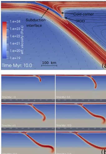
and continuously entrained into the decoupling region. The WL approach enables a mobile trench while also helping to accommodate plate bending, which is important in the ab-sence of a free surface. Additionally, it isolates the extremely weak parts of the system (the plate boundary) from the plates, enabling long-term asymmetric subduction to occur. In this study, we focus on a simple constant-viscosity implementa-tion of the WL using the Underworld2 code, as described in Sect. 2.
Although the WL is commonly implemented in numerical subduction models, there is some ambiguity as to whether this approach represents an attempt to explicitly model sub-duction interface dynamics, or should instead be conceived as an ad hoc solution to modelling the plate boundary. WL implementations do mimic several critical processes that are thought to contribute to the long-term weakness and stability of the subduction interface. One of these is the process of en-trainment or “self-lubrication” (Lenardic and Kaula, 1994). The entrainment of both sediments and fluids along the slab interface likely plays a key role in maintaining subduction interface weakness. Additionally, the WL approach might be linked with deformation-localizing processes such as dam-age, grain size reduction, and fabric development. Indeed, WL models have been conceived as a limiting case in which comprehensive damage is assumed within the interface mate-rial and hence can be prescribed at the outset (Tagawa et al., 2007). Despite the fact that we can draw analogies to relevant physical processes, our view is that the WL approach consti-tutes an ad hoc solution to the sub-grid phenomena of plate boundary shear localization.
The behaviour of the WL is discussed is some detail in Arcay (2012, 2017). These studies highlight the tendency for the subduction interface to develop spontaneous thickness variation as the models evolve. Typically the interface widens near the trench, building a prism-like complex, and thins at depths beyond the brittle–ductile transition (>50 km). This pattern was also noted in the boundary element models of Gerardi and Ribe (2018), who attributed a downdip thick-ness variation to lubrication layer dynamics. The tendency for thinning will impact the level of mesh resolution required in a model (Arcay, 2017). Additionally, WL formulations are likely to evolve maximum subduction interface thickness around twice the imposed thickness, potentially impacting effective stress along the interface, as well as the accuracy of predicted thermal structure. Understanding and control-ling these spontaneous width variations will be important in terms of using dynamic models to explore sensitive subduc-tion zone processes, such as metamorphism and melting near the slab top.
4 Methods
4.1 Numerical model setup
The numerical subduction models developed in this study represent the time evolution of simplified conservation equa-tions for mass, momentum, and energy within a 2-D Carte-sian domain. Figure 2 provides an overview of the model do-main, as well as initial and boundary conditions. The depth of the domain is 1000 km, and the aspect ratio is 5. Initial temperature conditions define two plates which meet at the centre of the domain, including a small asymmetric slab fol-lowing a circular arc to a depth of 150 km. The subducting plate has an initial age of 50 Myr at the trench, while the up-per plate age is 10 Myr. Both plates have a linear age profile with an initial age of zero at the sidewalls. This setup al-lows the model to evolve under the driving force of internal density anomalies (sometimes referred to as a fully dynamic model). Apart from the presence of a WL, there is no compo-sitional difference between the subducting and upper plate, nor do we include any compositional differentiation within the oceanic lithosphere. The only aspects of the model setup that are varied are the details of subduction interface imple-mentation (described in the following section) and the model resolution.
The mantle is treated as an incompressible, highly viscous fluid in which inertial forces and elastic stresses can be ne-glected. The mechanical behaviour of mantle (including the thermal lithosphere) is prescribed by a composite rheological model that includes a linear high-temperature creep law, as well as a scalar visco-plastic flow law, sufficient for captur-ing pseudo-brittle as well as distributed plastic deformation within the slab. Thermal buoyancy is the only source of den-sity variation in the model. The thermal variations are cou-pled to the momentum equation through their effect on den-sity, which follows the Boussinesq approximation. A detailed description of the governing equations, constitutive laws, and physical parameters is given in Appendix A.
Approximate solutions to the incompressible momentum and energy conservation equations are derived using the finite-element code Underworld2. Underworld2 is a Python API which provides functionality for the modelling of geo-dynamic processes. Underworld2 solves the discrete Stokes system through the standard mixed Galerkin finite-element formulation. The domain is partitioned into quadrilateral el-ements, with linear elements for velocity and constant ele-ments for pressure (Q1/dP0) (Arnold and Logg, 2014).
Figure 2.Initial conditions for 2-D thermo-mechanical subduction models. All models in this study have a 50 Myr initial slab age. Velocity boundary conditions are free slip on all walls of the domain (zero tangential stress). The dark grey region in the main panel shows parts of the model colder than 1100◦C. The inset shows the full domain. Outlines show the slab position at 10 and 20 Myr. The right-hand panel shows the viscosity profile evaluated along the vertical dashed line in the main panel.
used to distinguish the subduction interface material from the rest of the system (lithosphere and mantle). Underworld2 solves the energy conservation equation using an explicit streamline upwind Petrov–Galerkin (SUPG) method (Brooks and Hughes, 1982). In this approach, a Petrov–Galerkin for-mulation is obtained by using a modified weighting function which affects upwinding-type behaviour. The Stokes system has free-slip conditions on all boundaries. The energy equa-tion has constant (Dirichlet) and zero-flux (Neumann) on the top and bottom boundaries respectively. The left and right sidewalls have a constant temperature equal to the mantle potential temperature (1673 K). The surface temperature is 273 K.
4.2 Subduction interface implementation
The focus of our study is a common approach to modelling the subduction interface, sometimes referred to as a weak layer or weak crust. This approach has two intrinsic fea-tures: (1) the material that provides decoupling within the interplate zone is a distinct material type with rheology that contrasts with the plates/background material, and (2) the weak material layer is distributed along some or all of the subducting plate, so that the flow itself entrains new weak material into the decoupling region (Billen and Hirth, 2007; Garel et al., 2014; ˇCížková and Bina, 2013; Arredondo and Billen, 2017; Agrusta et al., 2017). In this study we use the abbreviation WL to refer to a typical implementation, namely one in which the distribution of weak material is fully self-evolving within the deforming subduction interface zone. We also demonstrate a modified version of this approach, which we refer to as an embedded fault (EF). The EF implemen-tation differs from the WL in that the width of the inter-face is constrained in terms of its minimum and maximum thickness. While this manipulation of the interface material could be achieved in different ways, our implementation is based on a reference line of particles, which lie at the base of the weak interface and are advected along with the material swarm. At each time step we remap material types based on
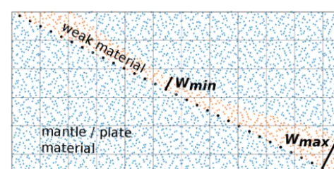
Figure 3.Schematic of the embedded fault (EF) implementation. The EF is a modification to the standard weak layer approach (WL). As with the WL, shear localizes due to a finite-width layer of weak material (represented by orange particles). A reference line of tracer particles (black points) is advected with the flow, at the base of the weak material layer. This line provides a reference to enforce width limits on the weak material, denoted byWminandWmax. At each time step we remap material types based on the relative position of the material particles to the reference line. Note that the element size here is not shown to scale.
the relative position of the material particles with regard to the reference line.
The relationship between the EF reference line, the mate-rial swarm, and the mesh is shown in Fig. 3. In the EF ap-proach, we also initialize the interface with a non-uniform thickness. For reasons discussed in the following sections, the thickness of the interface material within the decoupling zone should be close to double the thickness that is pre-scribed on the top of the subducting plate.
It is important to emphasize that differences between the WL and EF implementations relate only to the distribution of weak material within the model. All other aspects of the interface representation remain identical. In each case the in-terface has a constant viscosity. Weak material is continually prescribed along the uppermost part of the subducting plate as it moves away from the ridge, with a specified constant thickness (Winit=10 km). The upper plate does not contain
rhe-ological variation between the shallow (frictional) megath-rust and the deeper, viscous interface. To control the upper limit of the MDD, a depth-dependent cosine taper is used to transition the subduction interface rheology to the back-ground mantle rheology. The taper for the transition (both WL and EF) begins at 100 km, and has a width of 30 km. De-coupling is strongly inhibited at depths greater than the taper onset. Hence the depth of the taper onset (100 km) effectively controls the upper limit of MDD. Likewise, at a distance of 800 km from the trench, along the subducting plate, the rheology of the interface material transitions to background mantle rheology. This avoids interaction of weak material with the spreading ridge.
5 Analysis of modelling approaches 5.1 The weak layer approach
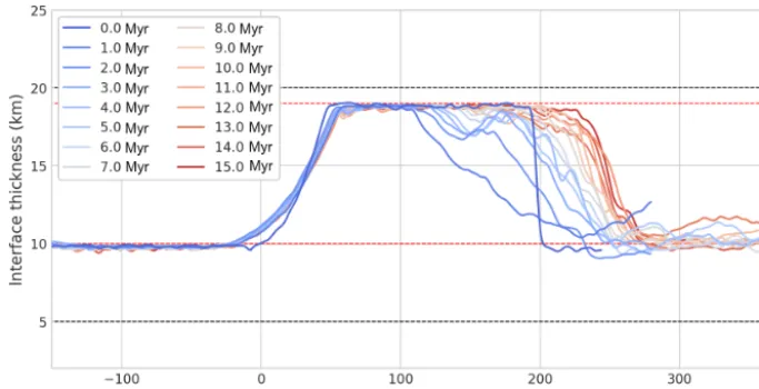
Figure 4 shows the evolution of the subduction interface thickness over a 20 Myr period, based on the WL setup scribed in Sect. 4. This model reveals the spontaneous de-velopment of substantial WL thickness variations, not only near the trench (i.e. near the accretionary prism) but through-out the entirety of the decoupling zone. Previous studies have commented on the occurrence of similar thickness variations (Arcay, 2017; Gerardi and Ribe, 2018), although their ori-gin has not been closely considered. We propose that such variations arise primarily from the way that the kinematics of the flow in the WL effect the downdip volumetric flux. In the following discussion we refer to a slab-based coor-dinate system in a fixed upper plate reference frame, where
ˆ
y is the direction orthogonal to the slab midplane,sˆ is the direction parallel to the slab midplane, and the plate conver-gence velocity is equal to the subducting plate velocity (Vs).
Before reaching the trench, the WL material travels with the subducting plate, with near-uniform velocity and negligible shear (∂Vs
∂yˆ ≈0). In the subduction interface zone, however, the WL material decouples the slab and upper plate, and ve-locity gradients across the interface are finite. For a New-tonian rheology, the gradient is expected to be linear with
∂Vs
∂yˆ ≈
Vs
W (i.e. Couette flow). This change in velocity profile
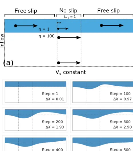
across the WL means that there is a smaller volumetric flux (per unit length normal to the interface) compared to the flux of material being delivered on the incoming subducting plate. To illustrate this point we consider a simple boundary-driven Stokes flow, as shown in Fig. 5, which provides a useful anal-ogy to the flow in the WL. In this model, flow is driven by a constant tangential velocity on the lower boundary, while the upper boundary of the model has a patch of frictional (no slip) nodes, surrounded on both sides by a free-slip boundary condition. The step change in boundary conditions imposes volumetric flux gradients causing the weak layer (shown in blue) to thicken near the start of the no-slip region, and thin
near the end. The width changes in the weak layer proceed until the overall volume flux reaches equilibrium.
Returning to our subduction model results, the validity of our description can be tested by considering the thickness profile required for volume flux equilibrium. Assuming that the decoupling zone maintains a Couette profile, independent of the local thickness, flux equilibrium requires that the thick-ness of the WL in the decoupling zone be twice that imposed on the incoming plate. This prediction, based on a simpli-fied kinematic description of flow in the interface, is broadly consistent with the long-term evolution observed in the WL models (e.g. Fig. 4).
While our discussion so far has mainly emphasized the transition of the WL from the oceanic part of the subducting plate into the decoupling zone, similar processes take place where the slab and the mantle become coupled (the MDD). When a constant interface width is prescribed, the interface thickness near the MDD initially decreases. Again, this is be-cause the volumetric flux increases as Couette flow in the de-coupling region transitions to the fully coupled flow. The lo-cation where the subduction interface thins provides a proxy for the MDD. Complexity arises due to the fact that the MDD in our model is not constant. Instead the MDD tends to be-come deeper as the corner of the mantle wedge cools and stagnates. This means that the effective boundary conditions on the flow within the interface are also time varying. This accounts for why the location of interface thinning migrates downdip as time progresses, as shown in Fig. 4.
Based on analysis of the typical WL setup, we argue that the primary thickness variations reflect a simple response to changes in volumetric flux along the interface. In addition to these flux-controlled changes, Fig. 4 shows that the sub-duction interface also develops a persistent short-wavelength width perturbation just beneath the tip of the forearc at a downdip distance of∼60–80 km. Here the interface thins by ∼3–4 km. This occurs in combination with strong, localized plastic deformation in the upper plate.
It seems likely that such short-wavelength anomalies may be affected by a range of factors, including the interface and lithosphere rheology, mesh resolution, and material advec-tion scheme. If so, these features are likely to be somewhat model dependent, in contrast to the long-wavelength, flux-related thickness variations which reflect intrinsic kinematics of flow in the WL setup.
5.2 Improving the weak layer approach
Figure 4.Interface thickness evolution in WL implementation. The initial layer thickness (Winit) is 10 km. Coloured lines show the evolving thickness plotted as a function of downdip distance from the trench. Dashed black lines show the expected maximum (equilibrium) and minimum (transient) thickness, based on a kinematic description of the flow evolving from a uniform thickness weak layer.
Figure 5.Analogue for WL thickness evolution.(a)Model setup for a boundary-driven flow where a weak layer (shown in blue) in-teracts with a stronger layer (white). The top surface of the model is free slip, except for a patch of no-slip nodes (Vx=0). The bottom
surface has a constant horizontal velocity component.(b)Evolution of material in the boundary-driven model.1X represents the ac-cumulated displacement along the bottom boundary, normalized by the width of the no-slip patch.
in some ways be a desirable approach, doing so results in the development of a very spurious subduction morphology. Figure 6b shows results from such a case (Wmax=Wmin=
Winit=10 km). After 15 million years of model evolution
a very atypical subduction morphology has developed, with an extremely low-angle megathrust beneath a forearc region with a width of greater than 600 km. While geologically irrel-evant, the example shown in Fig. 6b provides a useful insight into the way in which the flow in the interface can influence model dynamics. When the subduction interface is forced to remain at constant width, the interface is unable to evolve towards flux equilibrium. Persistent interface-normal veloc-ity components result, and the compounding effect eventu-ally distorts the morphology of the entire subduction hinge region.
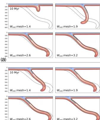
Figure 6a shows the slab morphology developed by instead usingWmax=1.9×Winit=19 km (we discuss the choice of
1.9 in the next section). The subduction morphology in this simulation is more realistic, and consistent with outcomes from a standard WL approach. The evolution of the interface thickness from the same simulation is shown in Fig. 8. In addition to controlling the width of the interface throughout the EF simulation, we have also prescribed the initial inter-face thickness in the decoupling zone (from the trench to a depth of 100 km) to have value equal toWmax(19 km). In this
condi-Figure 6. Effect of variable maximumWmaxin EF models. The colour map shows the effective viscosity at a model time of 10 Myr. White lines show isotherms at 700 and 1200◦C. Panel(a)shows the EF model withWmax=1.9×Winit=19 km. Panel(b)shows the EF model withWmax=Winit=10 km. In this case, due to the fact that the subduction interface cannot adjust its thickness, an ex-tremely long, low-angle interface develops, with forearc distances of∼500 km.
tions that include the cold corner would be one way to fur-ther reduce the amount the transient adjustment of the inter-face. Figure 7 shows the state of the material swarm in the EF model, compared to the equivalent WL model. This re-veals a typical distribution of interface material once a quasi-equilibrium thickness has been established.
In addition to the thickness variations related to volumetric flux, the WL approach can develop short wavelength thick-ness variations, as seen in Fig. 4. In the EF implementa-tion, we found that using a value ofWmaxslightly less than
2.0×Winithelps to suppress short wavelength thickness
vari-ations, without significantly effecting the overall model evo-lution. In other words, while we need to allow the interface to develop some amount of thickness variation, it may be ad-vantageous to use a value slightly less than 2×Winit.
Fig-ure 10 shows results from a number of experiments where the value of Wmaxwas changed. Qualitatively, we see that
the models have very similar long-term evolution onceWmax
is greater that 1.75×Winit.
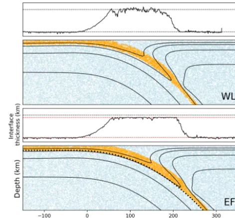
Figure 7. Distribution of subduction interface material. Results from a standard WL model are shown in the top panel. The EF model is shown in the bottom panel. Both models have a con-stant viscosity interface rheology. Model time is 12.5 Myr in both cases. In the lower panels, orange points are the subduction inter-face material, and blue points are the background material (man-tle/lithosphere). Points in the material swarm and along the EF ref-erence line have been down-sampled for clarity. Solid black lines over the material points are isotherms. Smaller panels show the measured interface thicknesses in each case; red horizontal lines show the thickness constraintsWmin,Wmax.
5.3 Stability and convergence
So far we have discussed results based on well-resolved mod-els, with 160 elements across the 1000 km vertical domain. At this resolution, the vertically refined mesh provides 3.2 elements within the subduction interface (atWinit=10 km).
Note that this increases to more than six elements in the de-coupling zone, once the interface has thickened to∼20 km. We now look at the convergence of models under variable resolution, based on a standard WL approach as well as the EF implementation. Figure 11 shows the slab temperature field at 10 Myr for a set of models with varying resolution: 72, 96, 128, 160, and 192 elements in the vertical dimen-sion. The ratio of the initial interface width (Winit) to the
Figure 8.Interface thickness evolution, EF approach. In the EF implementation limits are imposed in the maximum and minimum thick-nesses, as shown by the red dashed lines. Unlike the standard WL approach, the initial thickness of the interface is variable. The initial thickness of the interface within the decoupling region is equal toWmax. The black lines show the typical range in which a WL model will vary, assuming a constant initial thickness of 10 km (see also Fig. 4). The results shown here refer to the same model as shown in Figs. 1 and 6.
Figure 9.Evolution of the maximum depth of decoupling (MDD). As the mantle wedge cools, it progressively stagnates, driving deeper decoupling within the subduction interface. The grey region in the figure shows the depth interval over which the subduction in-terface transitions to the background mantle rheology as prescribed with a cosine taper (see Sect. 4). Results are from the same model as shown in Fig. 6a, i.e. an EF model withWmax=1.9×Winit.
decay. At 96 elements, the model is still strongly impacted by under-resolution of the subduction interface. Figure 11b shows equivalent results using the EF implementation. Qual-itatively, we see that EF models are more stable at lower res-olution. For instance, the EF model at the lowest resolution (72 elements) more closely reproduces the evolution of the reference model than does the WL model with 96 elements.
Figure 11 suggests that the EF models converge more closely with increasing resolution. We quantify this by track-ing the relative error (L2) of the temperature field in the
lower-resolution models with respect to the reference model (192 elements). The relative error with respect to the
refer-ence model (Tref) is
E=
R
(T−Tref)·(T−Tref)dV
R
Tref·TrefdV
1/2
. (1)
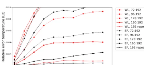
Figure 13 shows relative error results for the same set of models shown in Fig. 11, confirming more rapid resolution convergence in the EF models relative to the standard WL approach. For most of the models shown in Fig. 13 the rela-tive error accumulates rapidly in the first 7–10 million years of the simulation, while the error rate flattens after this. This is similar to the time taken for the WL interface to reach its equilibrium thickness (e.g. Fig. 4). This suggests that models are strongly resolution-sensitive during the transient phase of the interface adjustment. At low resolution (72, 96, 128 ele-ments), errors in both WL or EF models express this sensitiv-ity. Interestingly, at 160 elements, the EF case exhibits nearly constant error accumulation during the model evolution. This suggests that we have succeeded in reducing the sensitivity of the subduction interface implementation, relative to the overall error accumulation rate. The latter may be influenced by additional factors which we have not controlled for here, such as the time step size in the advection–diffusion imple-mentation which is controlled by the mesh resolution.
Figure 10.Embedded fault models (EF) with variableWmax. Lines show the morphology of the base of the subduction interface (the EF reference line) at 10 Myr for different models with varyingWmax. When the interface thickness variation is strongly constrained, the evolution of the model is significantly effected. See also Fig. 6.
Figure 12.Interface thickness in under-resolved WL model. In the lower panel orange points show the subduction interface material, and blue points are the background material (mantle/lithosphere). The upper panel shows interface thickness. This figure shows the model state 10 Myr after model initiation. This model is also shown in the upper left panel of Fig. 11a.
Figure 13.Convergence of models with varying resolution. Vertical axis shows the relative error (L2) of the temperature field. We have truncated the vertical axis so as to focus on trends in the higher-resolution results. The error value is based on the error between the highest-resolution model (192 elements in the vertical axis) and each of the models with lower resolution, as labelled in the figure. Experiments were repeated at the highest resolution to provide a baseline for model reproducibility (labelled “repeat”).
approach provides stability in this context, by inhibiting the feedback cycle. While this behaviour is mainly relevant for models run at low resolution, the increased stability of the EF approach is a useful property, particularly from a model development perspective.
6 Discussion and conclusions
The entrained weak layer (WL) is a common approach for implementing the subduction interface in long-term dynamic simulations. We have discussed aspects of WL implementa-tion that can have an unintended impact on model evoluimplementa-tion. The first involves the transient evolution of a uniform thick-ness interface to a variable thickthick-ness–uniform flux configu-ration. If not properly accounted for, thinning of the deeper
In general, models with plastic/frictional rheologies should be less sensitive to these transient adjustments, as the stress should not depend on the width of the interface.
Another tendency of the WL models is to develop persis-tent short-wavelength thickness variations. These may repre-sent interface instabilities, as are observed in Couette flows past a deformable boundary (Shankar and Kumar, 2004). These tend to dominate on the shallow part of the bound-ary with the upper plate. While flux-related thickness varia-tion will be expected for any model implementavaria-tion of WL, boundary instabilities (short wavelength) are likely to be more variable across different codes. They may depend on additional details of implementation, such as the rheology of the plates, material advection, and interpolation schemes. Together, these issues are likely to hinder efforts to produce reproducible results between codes.
These unintended behaviours of the WL approach can be partly mitigated by controlling the thickness of the interface. We demonstrate a simple implementation of this concept, which utilizes a line of reference points at the base of the WL, allowing us to remap material types based on proximity to this line. We call this approach an embedded fault (EF). The ability to constrain the thickness of the interface im-proves the resolution convergence of numerical models, as well as the stability at lower resolutions. The EF does add complexity to models, in both the sense of implementation as well as the introduction of new parameters to control specific details (e.g.Wmax). There are obviously other
implementa-tion strategies that could be developed in order to achieve similar outcomes. These should be explored in future stud-ies. Overall, this study provides a better understanding of the behaviour of subduction models utilizing WL approaches. These insights offer a basis for achieving better outcomes in terms of model reproducibility and precision.
Appendix A: Governing equations, constitutive relationships, and physical parameters
A1 Continuity, momentum, and energy equations On geological timescales the Earth’s mantle behaves as a highly viscous, incompressible fluid, in which inertial forces can be neglected. The flow caused by internal buoyancy anomalies is described by the static force balance (momen-tum conservation) and continuity equations:
σij,j+ρgi=0, (A1)
ui,i=0, (A2)
whereui is theith component of the velocity. Repeated
in-dices denote summation, andu,i represents partial derivative
with respect to the spatial coordinatexi. The full stress
ten-sor appearing in Eq. (A1) can be decomposed into deviatoric and mean components:
σij =τij+pδij. (A3)
It is noted that sign of the pressure (p) is opposite to the mean stress tensor, consistent with the convention that fluid flows from high to low pressure. The deviatoric stress tensor (τ) and the strain rate tensor (Dij) are related according to the
constitutive relationship:
τij=2ηDij=η(ui,j+uj,i). (A4)
Substituting Eqs. (A4) and (A3) into Eq. (A1) gives the Stokes equation, which involves two unknown variables: pressure and velocity. The Stokes and continuity equations are sufficient to solve for the two unknowns, together with appropriate boundary conditions. An approximate solution to these equations is derived using a Galerkin finite-element method, implemented in the Underworld2 code.
The thermal evolution of the system expresses the balance between heat transport by fluid motion, thermal diffusion, and internal heat generation by the first law of thermody-namics, assuming incompressibility:
ρCp
DT
Dt =qi,i+ρQ, (A5) whereT is the temperature andQis the heat production rate (everywhere zero in this study). Diffusion rates are described by Fourier’s law, which satisfies the second law for positive conductivity (k):
qi= −kT,i. (A6)
Inserting Eq. (A6) into Eq. (A5) and using the definition of the material derivative gives
∂T
∂t +uiT,i=(κT,i),i+ Q Cp
, (A7)
whereκ= k
ρCp is the thermal diffusivity.
The thermal variations are coupled to the momentum equation through their effect on density. At pressures in plan-etary interiors, silicate minerals are weakly compressible and this is generally considered to be a perturbation to an incom-pressible flow. The Boussinesq approximation accounts for the buoyancy forces while neglecting the associated volume change, allowing us to assume incompressibility (Eq. A2). In the case of density variations due to temperature, the equa-tion of state is
ρ=ρ0(1−α(T−Tp)), (A8)
whereρ0is the density at a reference temperature (here the
mantle potential temperatureTp).αis the coefficient of
ther-mal expansion. It is generally much sther-maller than 1, making the Boussinesq approximation reasonable.
The equations and parameters that appear in the numeri-cal models are based on equivalent dimensionless forms of the governing equations. We use the following characteristic scales (e.g Christensen, 1984):
xi=xi
1 d
, ui=ui d κ , η=η 1 η0 , τ=τ d2 κη0 ,
t=thκ d2
i
, T =T
1
1T
, (A9)
whered is the mantle depth,t is time,η0 is the reference
viscosity, and1T =(Ts−Tp)is the superadiabatic
temper-ature difference across the fluid layer. Substituting dimen-sional terms for scaled dimensionless values (e.g x→xd) and rearranging allows us to write the Stokes equation as 2ηDij,j+p,i=Ra(1−T )(−δiz). (A10)
Overbars in Eq. (A10) represent dimensionless quantities, and all dimensional parameters are contained in the dimen-sionless ratioRa, the Rayleigh number which can be inter-preted as a ratio of advection and diffusion timescales:
Ra=ρ0gα1T D
3
η0κ
. (A11)
The dimensionless viscosity, which has a functional de-pendence on the total pressure, the temperature, and the sec-ond invariant of the stress tensor, is described below.
The dimensionless form of the heat conservation equation is
∂T
∂t +uiT,i=(T,i),i+Q, (A12)
where the dimensionless internal heating is given by
Q=Q
d2
κCp1T
is independent of grain size. In addition to high-temperature creep, some form of stress-limiting behaviour is expected to occur at low temperature, and high stress. Glide-controlled dislocation creep (or Peierls creep), which includes a stress dependence of the activation energy, is likely to play a role, particularly in the cold part of subducted slabs (Karato, 2012). Nevertheless, it remains unclear whether Peierls creep allows sufficient weakening, as geophysical constraints on slabs would imply (e.g. Jain et al., 2017; Krien and Fleitout, 2008; Alisic et al., 2010). In geodynamic calculations, the effect of the Peierls mechanism is similar to that of plastic, temperature-independent plasticity models (Agrusta et al., 2017; Garel et al., 2014; ˇCížková and Bina, 2013).
To keep the models as simple as possible we include two deformation mechanisms: grain-size-independent diffusion creep and a plastic yielding based on a truncated Drucker– Prager plasticity model. The plastic strain rates are capable of representing brittle failure at low pressure (near the sur-face) and low-temperature plasticity at high pressure (deep within the slab). The value of the yield stress limit is chosen on the basis of previous studies, and is consistent with several lines of evidence suggesting that slabs do not support more than a few hundred megapascals (Richards et al., 2001; Tack-ley, 2000; Watts and Zhong, 2000; Krien and Fleitout, 2008; Alisic et al., 2010). The viscosity associated with each defor-mation mechanism is combined using a harmonic average, denoted byηc. The entire computational domain, except for
the subduction interface, is governed by the same composite rheology: there is no compositional distinction between the mantle and plates.
Ductile flow laws for silicates often have an Arrhenius temperature and pressure dependence, controlled by the acti-vation energyE, and activation volumeV (Hirth and Kohlst-edt, 2004). Additional dependencies, such as grain size and melt fraction, are neglected in this study, resulting in the fol-lowing diffusion viscosity:
ηd=Aexp
E+plV
RTa
, (A14)
whereplindicates the lithostatic component of the pressure,
andAis a constant. A linearized adiabatic term is added to the dimensionless temperature field, whenever it appears in an Arrhenius law.
Ta=T +z×T,z
T,z=
−αgTp
Cp
the dimensionless diffusion creep viscosity can be written
ηd=Aexp E+zW Ts+Ta
!
, (A16)
wherezis the dimensionless depth andTsis the
dimension-less surface temperature. The dimensiondimension-less linearized adia-batic component is incorporated as follows.
Ta=T +z×T,z
T0
,z=T,z
d
1T
The parameters chosen for the diffusion creep law are con-sistent with those derived from experimental data on dry olivine (Karato and Wu, 1993), providing an average upper mantle viscosity close to 1×10²⁰Pa s. The relatively high value of the activation volume produces relatively low vis-cosity asthenosphere∼0.3×10²⁰, relative to the transition zone∼5×10²⁰. Additionally, a viscosity increase (×η660)
is applied at the 660 km discontinuity, consistent with in-ferences based on the geoid (Hager and O’Connell, 1981). For (×η660=10), the lower mantle just beneath 660 km is
50 times more viscous than the mean viscosity of the up-per mantle. The parameters chosen produce radial viscosity profiles that are slightly higher than the “Haskell constraint” (ηmean=1×10²¹) over the upper 1400 km of the mantle (e.g.
Becker, 2017).
A range of pseudo-brittle and plastic deformation mecha-nisms can be approximated in the fluid constitutive model by allowing non-linearity in the viscosity (η=η(T , p, JI, . . .)).
The rheological model itself should be defined independently of the coordinate system, so it is necessary to define the con-stitutive model in terms of stress invariants (JI). The
stan-dard viscoplastic approach (Spiegelman et al., 2016) defines an effective plastic viscosityηpsuch that the deviatoric stress
tensor is bounded by a yield stressτy:
τy=2ηpDij. (A17)
Assuming thatηpis isotropic and scalar (i.e. eigenvectors
of the strain-rate tensor and deviatoric stress are identical), one can use the magnitude of both sides to define the scalar effective plastic viscosity as
ηp=
τy(II)
2II
, (A18)
The yield stress function in the computational models is a truncated Drucker–Prager criterion:
τy=min(τmax, µp+C), (A19)
whereµis the friction coefficient, andCis the cohesion. The Drucker–Prager yield surface is defined by the full pressure p. Because the pressure that appears in the dimensionless Stokes equation (Eq. A10) is a dynamic pressure (p), due to density variations only, the lithostatic pressure (a function of vertical coordinate) needs to be accounted for. The dimen-sionless form of the yield stress is given by
τy=min(τmax, µ(p+plz)+C), (A20)
where
µ=µ, C=C
d2 κη0
,
τmax=τmax d2
κη0
,
Pl=z
ρ 0gd3
κη0
. (A21)
The effective plastic viscosity (dimensionless) is given by ηp=τy(II)
2˙II
. (A22)
The final (composite) viscosity is the harmonic average of the viscosity associated with creep and plastic yielding
ηc= ηdηp
ηd+ηp. (A23)
A3 Model parameters and scaling values
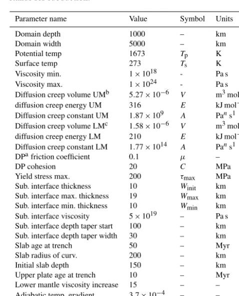
This section provides a record of model parameters and ref-erence values that are used in the models. The dimensional parameters quoted here are non-dimensionalized using the scaling system described in Appendix A and reference val-ues provided in Table A1. This scaling system is identical for all models used within the thesis.
Table A1.Reference values used to non-dimensionalize the Stokes and energy equations, as described in Appendix A.
Reference value Value Symbol Units
Length 2900 d km
Viscosity 1×10²⁰ η0 Pa s
Density 3300 ρ0 kg m−3
Thermal diffusivity 1×10⁻⁶ κ m2s−1
Gravity 9.8 g m s−2
Temperature 1400 1T K
Gas constant 8.314 R J mol−1K−1
Rayleigh number 3.31×10⁸ Ra –
Table A2.Typical model element resolution was 800×160. Sub. stands for subduction.
Parameter name Value Symbol Units
Domain depth 1000 – km
Domain width 5000 – km
Potential temp 1673 Tp K
Surface temp 273 Ts K
Viscosity min. 1×10¹⁸ - Pa s
Viscosity max. 1×1024 - Pa s
Diffusion creep volume UMb 5.27×10⁻⁶ V m3mol−1 diffusion creep energy UM 316 E kJ mol−1 Diffusion creep constant UM 1.87×10⁹ A Pans1 Diffusion creep volume LMc 1.58×10⁻⁶ V m3mol−1 diffusion creep energy LM 210 E kJ mol−1 Diffusion creep constant LM 1.77×10¹⁴ A Pans1
DPafriction coefficient 0.1 µ –
DP cohesion 20 C MPa
Yield stress max. 200 τmax MPa
Sub. interface thickness 10 Winit km
Sub. interface max. thickness 19 Wmax km
Sub. interface min. thickness 10 Wmin km Sub. interface viscosity 5×10¹⁹ – Pa s Sub. interface depth taper start 100 – km Sub. interface depth taper width 30 – km
Slab age at trench 50 – Myr
Slab radius of curv. 200 – km
Initial slab depth 150 – km
Upper plate age at trench 10 – Myr
Lower mantle viscosity increase 15 – – Adiabatic temp. gradient 3.7×10⁻⁴ – –
Internal heating 0.0 Q W m−3
Acknowledgements. The study benefited from the authors’ atten-dance of the CIDER summer programs in 2016 and 2017 (funded by NSF grant EAR-1135452). This work was supported by re-sources provided by the Pawsey Supercomputing Centre with fund-ing from the Australian government and the government of West-ern Australia. This research was supported by use of the Nectar Research Cloud, a collaborative Australian research platform sup-ported by the National Collaborative Research Infrastructure Strat-egy (NCRIS).
Financial support. This research has been supported by the Centre of Excellence for Core to Crust Fluid Systems, Australian Research Council (grant no. DP150102887). Dan Sandiford’s postgraduate research at the University of Melbourne was supported by a Barag-wanath Geology Research Scholarship.
Review statement. This paper was edited by Taras Gerya and re-viewed by Hana Cizkova, Thibault Duretz, and one anonymous ref-eree.
References
Aagaard, B., Knepley, M., and Williams, C.: PyLith v2.2.1, Computational Infrastructure for Geodynamics, https://doi.org/10.5281/zenodo.886600, 2017.
Abers, G. A.: Seismic low-velocity layer at the top of subduct-ing slabs: observations, predictions, and systematics, Phys. Earth Planet. Int., 149, 7–29, 2005.
Agrusta, R., Goes, S., and van Hunen, J.: Subducting-slab transition-zone interaction: Stagnation, penetration and mode switches, Earth Planet. Sc. Lett., 464, 10–23, 2017.
Alisic, L., Gurnis, M., Stadler, G., Burstedde, C., Wilcox, L. C., and Ghattas, O.: Slab stress and strain rate as constraints on global mantle flow, Geophys. Res. Lett., 37, L22308, https://doi.org/10.1029/2010gl045312, 2010.
Androviˇcová, A., ˇCížková, H., and van den Berg, A.: The effects of rheological decoupling on slab deformation in the Earths upper mantle, Stud. Geophys. Geod., 57, 460–481, 2013.
Arcay, D.: Dynamics of interplate domain in subduction zones: in-fluence of rheological parameters and subducting plate age, Solid Earth, 3, 467–488, https://doi.org/10.5194/se-3-467-2012, 2012. Arcay, D.: Modelling the interplate domain in thermo-mechanical simulations of subduction: Critical effects of resolution and rhe-ology, and consequences on wet mantle melting, Phys. Earth Planet. Int., 269, 112–132, 2017.
Geosci., 6, 852, 2013.
Audet, P., Bostock, M. G., Christensen, N. I., and Peacock, S. M.: Seismic evidence for overpressured subducted oceanic crust and megathrust fault sealing, Nature, 457, 76–78, 2009.
Babeyko, A. and Sobolev, S.: High-resolution numerical model-ing of stress distribution in visco-elasto-plastic subductmodel-ing slabs, Lithos, 103, 205–216, 2008.
Bachmann, R., Oncken, O., Glodny, J., Seifert, W., Georgieva, V., and Sudo, M.: Exposed plate interface in the European Alps re-veals fabric styles and gradients related to an ancient seismo-genic coupling zone, J. Geophys. Res.-Sol. Ea., 114, B05402, https://doi.org/10.1029/2008JB005927 2009.
Bayet, L., John, T., Agard, P., Gao, J., and Li, J.-L.: Massive sed-iment accretion at 80 km depth along the subduction interface: Evidence from the southern Chinese Tianshan, Geology, 46, 495–498, https://doi.org/10.1130/G40201.1, 2018.
Bebout, G. E. and Penniston-Dorland, S. C.: Fluid and mass transfer at subduction interfaces, The field metamorphic record, Lithos, 240, 228–258, 2016.
Becker, T. W.: Superweak asthenosphere in light of upper mantle seismic anisotropy, Geochem. Geophys. Geosy., 18, 1986–2003, 2017.
Behr, W. M. and Becker, T. W.: Sediment control on sub-duction plate speeds, Earth Planet. Sc. Lett., 502, 166–173, https://doi.org/10.1016/j.epsl.2018.08.057, 2018.
Bercovici, D.: The generation of plate tectonics from mantle con-vection, Earth Planet. Sc. Lett., 205, 107–121, 2003.
Bercovici, D. and Ricard, Y.: Plate tectonics
dam-age and inheritance, Nature, 508, 513–516,
https://doi.org/10.1038/nature13072, 2014.
Billen, M. I. and Hirth, G.: Rheologic controls on slab
dynamics, Geochem. Geophys. Geosy., 8, Q08012,
https://doi.org/10.1029/2007gc001597, 2007.
Billen, M. I., Gurnis, M., and Simons, M.: Multiscale dynamics of the Tonga-Kermadec subduction zone, Geophys. J. Int., 153, 359–388, 2003.
Brooks, A. N. and Hughes, T. J.: Streamline upwind/Petrov-Galerkin formulations for convection dominated flows with par-ticular emphasis on the incompressible Navier-Stokes equations, Comput. Method. Appl. M., 32, 199–259, 1982.
Capitanio, F., Stegman, D., Moresi, L., and Sharples, W.: Upper plate controls on deep subduction, trench migrations and de-formations at convergent margins, Tectonophysics, 483, 80–92, 2010.
Chertova, M. V., Geenen, T., van den Berg, A., and Spak-man, W.: Using open sidewalls for modelling self-consistent lithosphere subduction dynamics, Solid Earth, 3, 313–326, https://doi.org/10.5194/se-3-313-2012, 2012.
Christensen, U. R.: The influence of trench migration on slab pene-tration into the lower mantle, Earth Planet. Sc. Lett., 140, 27–39, 1996.
ˇ
Cížková, H. and Bina, C. R.: Effects of mantle and subduction-interface rheologies on slab stagnation and trench rollback, Earth Planet. Sc. Lett., 379, 95–103, 2013.
ˇ
Cıžková, H., van Hunen, J., van den Berg, A. P., and Vlaar, N. J.: The influence of rheological weakening and yield stress on the interaction of slabs with the 670 km discontinuity, Earth Planet. Sc. Lett., 199, 447–457, 2002.
Cloos, M. and Shreve, R. L.: Subduction-channel model of prism accretion, melange formation, sediment subduction, and subduc-tion erosion at convergent plate margins: 1. Background and de-scription, Pure Appl. Geophys., 128, 455–500, 1988.
Duarte, J. C., Schellart, W. P., and Cruden, A. R.: How weak is the subduction zone interface?, Geophys. Res. Lett., 42, 2664–2673, 2015.
Gao, X. and Wang, K.: Strength of stick-slip and creeping sub-duction megathrusts from heat flow observations, Science, 345, 1038–1041, 2014.
Garel, F., Goes, S., Davies, D. R., Davies, J. H., Kramer, S. C., and Wilson, C. R.: Interaction of subducted slabs with the mantle transition-zone: A regime diagram from 2-D thermo-mechanical models with a mobile trench and an overriding plate, Geochem. Geophys. Geosy., 15, 1739–1765, https://doi.org/10.1002/2014gc005257, 2014.
Gerardi, G. and Ribe, N. M.: Boundary-element modeling of two-plate interaction at subduction zones: scaling laws and applica-tion to the Aleutian subducapplica-tion zone, J. Geophys. Res.-Sol. Ea., 123, 5227–5248, https://doi.org/10.1002/2017JB015148, 2018. Gerya, T. V., Connolly, J. A., and Yuen, D. A.: Why is terrestrial
subduction one-sided?, Geology, 36, 43–46, 2008.
Glerum, A., Thieulot, C., Fraters, M., Blom, C., and Spak-man, W.: Nonlinear viscoplasticity in ASPECT: benchmark-ing and applications to subduction, Solid Earth, 9, 267–294, https://doi.org/10.5194/se-9-267-2018, 2018.
Gurnis, M. and Hager, B. H.: Controls of the structure of subducted slabs, Nature, 335, 317–321, 1988.
Hager, B. H. and O’Connell, R. J.: A simple global model of plate dynamics and mantle convection, J. Geophys. Res., 86, 4843, https://doi.org/10.1029/jb086ib06p04843, 1981.
Hardebeck, J. L.: Stress orientations in subduction zones and the strength of subduction megathrust faults, Science, 349, 1213– 1216, 2015.
Hardebeck, J. L. and Loveless, J. P.: Creeping subduction zones are weaker than locked subduction zones, Nat. Geosci., 11, 60–66, 2018.
Hirauchi, K.-i. and Katayama, I.: Rheological contrast between ser-pentine species and implications for slab–mantle wedge decou-pling, Tectonophysics, 608, 545–551, 2013.
Hirth, G. and Kohlstedt, D.: Rheology of the upper mantle and the mantle wedge: A view from the experimentalists, Inside the sub-duction Factory, 138, 83–105, 2004.
Holt, A. F., Buffett, B. A., and Becker, T. W.: Overriding plate thick-ness control on subducting plate curvature, Geophys. Res. Lett., 42, 3802–3810, 2015.
Huene, R. and Scholl, D. W.: Observations at convergent margins concerning sediment subduction, subduction erosion, and the growth of continental crust, Rev. Geophys., 29, 279–316, 1991.
Jain, C., Korenaga, J., and Karato, S.-i.: On the yield strength of oceanic lithosphere, Geophys. Res. Lett., 44, 9716–9722, 2017. Karato, S.-I.: Deformation of earth materials: an introduction to the
rheology of solid Earth, Cambridge University Press, Cambridge, 2012.
Karato, S.-i. and Wu, P.: Rheology of the upper mantle: A synthesis, Science, 260, 771–778, 1993.
Kimura, G., Yamaguchi, A., Hojo, M., Kitamura, Y., Kameda, J., Ujiie, K., Hamada, Y., Hamahashi, M., and Hina, S.: Tectonic mélange as fault rock of subduction plate boundary, Tectono-physics, 568, 25–38, 2012.
Kincaid, C. and Sacks, I. S.: Thermal and dynamical evolution of the upper mantle in subduction zones, J. Geophys. Res.-Sol. Ea., 102, 12295–12315, 1997.
Krien, Y. and Fleitout, L.: Gravity above subduction zones and forces controlling plate motions, J. Geophys. Res.-Sol. Ea., 113, B09407, https://doi.org/10.1029/2007JB005270, 2008.
Lamb, S.: Shear stresses on megathrusts: Implications for moun-tain building behind subduction zones, J. Geophys. Res.-Sol. Ea., 111, B07401, https://doi.org/10.1029/2005JB003916, 2006. Lenardic, A. and Kaula, W.: Self-lubricated mantle convection:
Two-dimensional models, Geophys. Res. Lett., 21, 1707–1710, 1994.
Li, B. and Ghosh, A.: Near-continuous tremor and low frequency earthquake (LFE) activities in the Alaska-Aleutian subduction zone revealed by a mini seismic array, Geophys. Res. Lett., 44, 5427–5435, https://doi.org/10.1002/2016GL072088, 2017. Magni, V., van Hunen, J., Funiciello, F., and Faccenna, C.:
Numeri-cal models of slab migration in continental collision zones, Solid Earth, 3, 293–306, https://doi.org/10.5194/se-3-293-2012, 2012. Manea, V. and Gurnis, M.: Subduction zone evolution and low vis-cosity wedges and channels, Earth Planet. Sc. Lett., 264, 22–45, 2007.
Moresi, L. and Solomatov, V.: Mantle convection with a brittle lithosphere: thoughts on the global tectonic styles of the Earth and Venus, Geophys. J. Int., 133, 669–682, https://doi.org/10.1046/j.1365-246x.1998.00521.x, 1998. Peacock, S. M.: Thermal and petrologic structure of subduction
zones, Subduction top to bottom, American Geophysical Union, 119–133, 1996.
Plank, T. and Langmuir, C. H.: Tracing trace elements from sedi-ment input to volcanic output at subduction zones, Nature, 362, 739–743, 1993.
Proctor, B. and Hirth, G.: Ductile to brittle transition in thermally stable antigorite gouge at mantle pressures, J. Geophys. Res.-Sol. Ea., 121, 1652–1663, 2016.
Reynard, B.: Serpentine in active subduction zones, Lithos, 178, 171–185, 2013.
Richards, M. A., Yang, W.-S., Baumgardner, J. R., and Bunge, H.-P.: Role of a low-viscosity zone in stabiliz-ing plate tectonics: Implications for comparative terrestrial planetology, Geochem. Geophys. Geosy., 2, 2000GC000115, https://doi.org/10.1029/2000GC000115, 2001.
namics, Geochem. Geophys. Geosy., 17, 2213–2238, 2016. Tackley, P. J.: Self-consistent generation of tectonic plates
in time-dependent, three-dimensional mantle convection sim-ulations, Geochem. Geophys. Geosy., 1, 2000GC000036, https://doi.org/10.1029/2000GC000036, 2000.
Tagawa, M., Nakakuki, T., Kameyama, M., and Tajima, F.: The role of history-dependent rheology in plate boundary lubrication for generating one-sided subduction, Pure Appl. Geophys., 164, 879–907, 2007.
Tichelaar, B. W. and Ruff, L. J.: Depth of seismic coupling along subduction zones, J. Geophys. Res.-Sol. Ea., 98, 2017–2037, 1993.
Trompert, R. and Hansen, U.: Mantle convection simulations with rheologies that generate plate-like behaviour, Nature, 395, 686– 689, https://doi.org/10.1038/27185 1998.
https://doi.org/10.1029/2011GC003846, 2012.
Vrolijk, P.: On the mechanical role of smectite in subduction zones, Geology, 18, 703–707, 1990.
Watts, A. and Zhong, S.: Observations of flexure and the rheology of oceanic lithosphere, Geophys. J. Int., 142, 855–875, 2000. Zhong, S. and Gurnis, M.: Viscous flow model of a subduction zone
with a faulted lithosphere: Long and short wavelength topog-raphy gravity and geoid, Geophys. Res. Lett., 19, 1891–1894, https://doi.org/10.1029/92gl02142, 1992.