Block-based cloud classiﬁcation with statistical features and distribution of local texture features

(1)

Atmos. Meas. Tech., 8, 1173–1182, 2015 www.atmos-meas-tech.net/8/1173/2015/ doi:10.5194/amt-8-1173-2015

Block-based cloud classification with statistical features and

distribution of local texture features

H.-Y. Cheng1and C.-C. Yu2

1_{Department of Computer Science and Information Engineering, National Central University, 300 Jongda Rd., Zhongli Dist.,} Taoyuan City 32001, Taiwan

2_{Department of Computer Science and Information Engineering, Vanung University, 1 Wanneng Rd., Zhongli Dist., Taoyuan} City 32061, Taiwan

Correspondence to: H.-Y. Cheng ([email protected])

Received: 5 September 2014 – Published in Atmos. Meas. Tech. Discuss.: 25 November 2014 Revised: 19 February 2015 – Accepted: 19 February 2015 – Published: 10 March 2015

Abstract. This work performs cloud classification on all-sky images. To deal with mixed cloud types in one image, we propose performing block division and block-based classi-fication. In addition to classical statistical texture features, the proposed method incorporates local binary pattern, which extracts local texture features in the feature vector. The com-bined feature can effectively preserve global information as well as more discriminating local texture features of different cloud types. The experimental results have shown that apply-ing the combined feature results in higher classification accu-racy compared to using classical statistical texture features. In our experiments, it is also validated that using block-based classification outperforms classification on the entire images. Moreover, we report the classification accuracy using dif-ferent classifiers including the k-nearest neighbor classifier, Bayesian classifier, and support vector machine.

1 Introduction

The demand for sustainable and green energy is growing as fossil fuel bases decline and gas emissions increase. Solar energy is one emerging green energy that has been improved significantly in recent years. Recently, a large number of pho-tovoltaics (PV) were installed worldwide. However, the main challenge of PVs is that the produced electricity is often vari-able and intermittent. The fluctuation of the supply makes the energy expensive and prevents it from prevalence. Due to the unpredictable nature, the grid operators usually need to adopt a more conservative strategy and reserve enough power. If the

reserved power is not used, it is a waste. If the reserved power is not enough, a blackout will happen. To utilize solar energy more effectively, integrated and large-scale PV systems need to overcome the unstable nature of solar resources. PV grid operators desire mechanisms of scheduling, dispatching, and allocating energy resources adaptively. Obtaining an accurate estimation of the resources that can be exploited is helpful for reducing costs and achieving better efficiency. Therefore, the ability to perform accurate short-term forecast on surface solar irradiance is desired.

(2)

1174 H.-Y. Cheng and C.-C. Yu: Block-based cloud classification

more refined scales is feasible. Such analysis on cloud activi-ties include cloud-cover detection, cloud tracking, and cloud classification. The purpose of cloud classification is to distin-guish the cloud types and hopefully figure out their impacts on the change of irradiance.

In the work of Martínez-Chico et al. (2011), the clouds were classified into different attenuation groups according to different levels of attenuation of the direct solar radia-tion reaching the surface. The authors also analyzed the an-nual and seasonal frequencies of each cloud group. However, this work did not propose any method for extracting features from images and performing classification based on image features. For works of cloud classification using sky image features, we review the following existing methods. The re-search by Calbo and Sabburg (2008) used features based on Fourier transform along with simple statistics such as stan-dard deviation, smoothness, moments, uniformity, and en-tropy. The features are extracted from intensity images and red-to-blue components ratio (R/B) images. The classifier they used was based on the supervised classification paral-lelepiped technique.

In the work of Heinle et al. (2010) statistical features such as mean, standard deviation, skewness, and difference are uti-lized. Also, textural features including energy, entropy, con-trast, and homogeneity are computed from the grey-level co-occurrence matrices (GLCM). Instead of extracting features from intensity images, the authors reported the color com-ponent for which each individual feature should be calcu-lated. This work used ak-nearest neighbor (k-NN) classifier to classify the clouds into seven different types. Kazantzidis et al. (2012) improved the method of Heinle et al. by dividing the data set into subclasses according to solar zenith angle, cloud coverage, and visible fraction of the solar disk. Other features such as autocorrelation, edge frequency, Law’s fea-tures, and primitive length are also tested for cloud classifi-cation (Singh and Glennen, 2005).

The statistical features utilized in these works are basic and simplified descriptors. The abilities of these descriptors are more restricted since a certain amount of information is lost in the simplification process. In addition to the simple statistical features, we extract the local texture features us-ing local binary patterns (LBPs) (Suruliandi et al., 2012). The texture information encoded by LBP forms higher di-mensional feature vectors compared to traditional statistical features. Therefore, we perform dimension reduction on the extracted feature vector before performing classification.

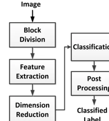
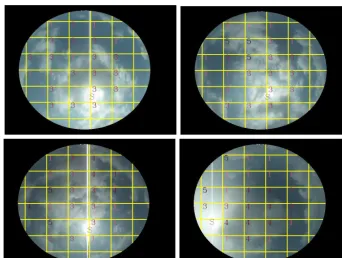
Figure 1 illustrates the proposed system framework. An all-sky image is divided into blocks before the features are extracted. The existing works classified the clouds based on the entire scene. However, very often there are mixed cloud types in the scene of an all-sky image as can be observed in Fig. 2. Therefore, we divide the scene into blocks and perform classification based on the feature of each block. After block division, the system extracts statistical and tex-ture featex-tures based on local patterns from each block. Then,

Figure 1. System framework.

principal component analysis (PCA) (Duda et al., 2001) is performed to reduce the dimensionality of the extracted fea-ture vectors. For classification, we compare several classi-fiers, including k-NN, Bayesian classifier with regularized discriminant analysis (Cheng et al., 2010), and support vec-tor machine (SVM) (Cristianini and Shawe-Taylor, 2000). In this work, the blocks are classified into cirrus, cirrostratus, scattered cumulus or altocumulus, cumulus or cumulonim-bus, stratus, and clear sky. In the post-processing step, the classification results from the classifier are examined using the cloud-cover information. Furthermore, a voting scheme is proposed to summarize the classified label of the entire image from the class labels of all the blocks.

2 Data and methodology

This section outlines the data sources and samples as well as the methodology used for classification.

2.1 All-sky images

The all-sky images used in this research are captured by the all-sky camera manufactured by the Santa Barbara Instru-ment Group. The charge-coupled device is Kodak KAI-0340. The lens of the camera is Fujinon FE185C046HA-1. The fo-cal length is 1.4 mm and fofo-cal ratio range is f/1.4 to f/16. The device covers a field of view of 185◦. The RGB images are stored in bitmap format with resolution 640×480. The data set is provided by the Industrial Technology Research Institute of Taiwan.

(3)

H.-Y. Cheng and C.-C. Yu: Block-based cloud classification 1175 5

82

Figure 1. System Framework

83 84

85

(a) (b)

86

Figure 2. Conditions of mixed cloud types. 87

88

2.Data and Methodology

89

This section outlines the data sources and samples as well as the methodology used for classification.

90

2.1 All Sky Images

91

The all sky images used in this research are captured by the all sky camera manufactured by the Santa

92

Barbara Instrument Group (SBIG). The charge-coupled device (CCD) is Kodak KAI-0340. The lens of the

93

camera is Fujinon FE185C046HA-1. The focal length is 1.4mm and focal ratio range is f/1.4 to f/16. The

94

device covers a field of view (FOV) of 185 degrees. The RGB images are stored in bitmap format with

95

resolution 640 x 480. The dataset is provided by the Industrial Technology Research Institute of Taiwan.

96

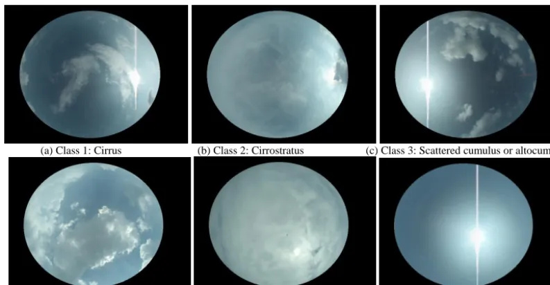
Figure 3 displays the six types of clouds that the system will perform classification. Cirrus clouds and

97

Figure 2. Conditions of mixed cloud types.

area of cirrostratus is larger. Altocumulus or scattered cu-mulus clouds are mid- to low-altitude clouds which look like blobs of cotton. Cumulus or cumulonimbus clouds are lower-altitude clouds which have noticeable vertical development and are often darker and larger. Stratus clouds are flat, wide-area clouds at lower altitude.

2.2 Block division

In practice, there might be more than one cloud type in one sky image, as shown in Fig. 2. In Fig. 2a, some cumulus clouds present in the scene, and there are some cirrostra-tus clouds around the sun area. In Fig. 2b, a cumulus cloud blocks the sun, and some altocumulus and cirrus clouds also exist in other regions of the image. Mixing up the features of cumulus, altocumulus, and cirrostratus clouds tends to con-fuse the classifier. Therefore, under such conditions of mixed cloud types, it is not appropriate to use the features of the entire image and classify the whole image as a certain cloud type. To solve this problem, we divide the entire scene into blocks and perform classification based on blocks. An exam-ple of the divided block is shown in Fig. 4 with block size 60×80 pixels. The feature vector of a block represents the characteristics of the cloud type in the block only. Such de-sign will reduce the confusing conditions of mixing up fea-tures of different cloud types. Additionally, we can obtain more detailed information about the location of each cloud type. This information is very helpful since the clouds in the regions closer to the sun have higher impact on the irradiance changes.

2.3 Feature extraction

This work combines the statistical features proposed in the work by Heinle et al. (2010) and the distribution of local tex-ture featex-tures using LBP codes (Suruliandi et al., 2012). The statistical features represent the spectral and texture informa-tion in a global view. On the contrary, the LBP codes encode the local characteristics of the gradient and texture features.

2.3.1 Statistical features

The statistical feature vector used in the work by Heinle et al. (2010) includes statistical spectral features and statisti-cal textual features. The statististatisti-cal spectral features include the following dimensions: mean ofRcomponents, mean of B components, standard deviation ofB component, skew-ness of B component, and differences ofR–G,R–B, and G–Bcomponents. The statistical textual features are statisti-cal measures computed from GLCM (Haralick et al., 1973), including energy, entropy, contrast, and homogeneity of the GLCM. Also, the cloud-cover ratio is considered as a fea-ture. The details of these statistical features can be found in the work by Heinle et al. (2010).

2.3.2 Distribution of local texture features

In addition to the above-mentioned statistical features, we enhance the texture features by applying LBPs (Suruliandi et al., 2012). The LBPP ,Rcode for a pixel(xc,yc)is defined in Eq. (1). In this equation,gcdenotes the grey-level value of the center pixel(xc,yc), andgpdenotes the grey-level value of its neighboring pixel. The parameterP sets the number of neighboring pixels that are considered when computing the binary codes. The parameterRsets the distance between the center pixel and its neighbors. For LBP8,1codes, we consider the eight neighboring pixels whose distance with the center pixel is 1. The code represents the local texture characteris-tics around(xc, yc).

LBPP ,R(xc, yc)=

P−1 X

p=0

s(gp−gc)2p (1)

s(gp−gc)=

1 gp−gc≥0 0 gp−gc<0

(4)

1176 H.-Y. Cheng and C.-C. Yu: Block-based cloud classification 6

cirrostratus clouds are high and thin clouds. The main difference between cirrus clouds and cirrostratus 98

clouds is that the area of cirrostratus is larger. Altocumulus or scattered cumulus clouds are middle to low 99

altitude clouds, which look like blobs of cotton. Cumulus or cumulonimbus clouds are lower- altitude clouds 100

which have noticeable vertical development and are often darker and larger. Stratus clouds are flat and 101

wide-area clouds at lower altitude. 102

103

(a) Class 1: Cirrus (b) Class 2: Cirrostratus (c) Class 3: Scattered cumulus or altocumulus 104

105

(d) Class 4: Cumulus or cumulonimbus (e) Class 5: Stratus (f) Class 6: Clear sky 106

Figure 3.Six different types 107

108

2.2 Block Division 109

In practice, there might be more than one cloud types in one sky image as shown in Figure 2. In Figure 2 (a), 110

some cumulus clouds present in the scene, and there are some cirrostratus clouds around the sun area. In 111

Figure 2 (b), a cumulus cloud blocks the sun, and some altocumulus and cirrus clouds also exist in other 112

regions of the image. Mixing up the features of cumulus, altocumulus, and cirrostratus tends to confuse the 113

classifier. Therefore, under such conditions of mixed cloud types, it is not appropriate to use the features of 114

the entire image and classify the whole image as a certain cloud type. To solve this problem, we divide the 115

entire scene into blocks and perform classification based on blocks. An example of the divided block is 116

Figure 3. Six different types.

Figure 4. Block division example.

histogram by voting with the codes of all the pixels in the region. The LBP histogram characterizes the distribution of local texture features of the region.

We apply the LBPP ,Rcodes withP =8 andR=1 to

ex-tract local texture features in this work. For LBP8,1 codes, there are 256 distinct values since the code is an 8 bit bi-nary number. Therefore, 256 histogram bins are required for all the distinct codes. However, it has been shown that some codes appear more frequently than others, concentrat-ing the votes in the histogram in a few bins. The codes that appear with higher frequencies are the uniform LBP codes. Researches have shown that uniform LBP codes account for over 90 % of all LBP codes. The uniform LBP codes are the codes that have at most two zero-to-one or one-to-zero

transi-tions. Among the 256 distinct LBP codes, 58 LBP codes are uniform. As a consequence, we can use 58 bins for the uni-form LBP codes and one extra bin for all the non-uniuni-form LBP codes in the histogram. In total, the number of his-togram bins is reduced to 59 instead of 256.

Because clouds of a certain type might be rotated, we fur-ther consider rotation invariant LBP code. To make the LBP code invariant to rotation, the code is circularly shifted to a minimum code number. In Eq. (3), ROR(LBPP ,R, i)

per-forms a circular bit-wise right shift on LBPP ,R for itimes.

For rotation invariant LBP, there are nine uniform patterns. Therefore, only 10 bins are required for the histogram of uni-form rotation invariant LBPs.

LBPRI_{P ,R}=min{ROR(LBPP ,R, i)|i=0, 1, · · ·, P−1} (3)

To obtain the distribution of the local texture patterns and to retain the localized information as well, we divide each block intoNcell cells when constructing the feature vector. One LBP histogram is generated for each cell. And then the Ncell histograms are concatenated to form the feature vec-tor. In other words, for each image block, we generate a 59×Ncelldimensional feature vector for uniform LBPs and a 10×Ncelldimensional feature vector for uniform rotation invariant LBPs.

2.3.3 Combining statistical features and distribution of local texture features

(5)

H.-Y. Cheng and C.-C. Yu: Block-based cloud classification 1177

LBP histogram. Since the statistical feature vector has 12 di-mensions, combined feature A and combined feature B have 12+59×Ncelland 12+10×Ncelldimensions, respectively. 2.4 Dimension reduction

PCA (Duda et al., 2001) is a commonly used way to re-duce the dimensions of the feature vectors. To rere-duce the dependency among different feature dimensions, PCA seeks to find a set of new orthogonal bases to re-express the data more effectively. The new orthogonal bases, which are called principal components, are linear combinations of the original bases. Considering the variability in the data as an impor-tant and desired characteristic, PCA will preserve most of the data variability to the first (often few) principal compo-nents. Suppose that the original data set X has D1 dimen-sions and there areN samples in the data set. The matrixX is aD1×N matrix whose columns are the original feature vectors. The PCA will select the first D2eigenvectors cor-responding to the first largestD2 eigenvalues of the matrix XTX, which is proportional to the empirical sample covari-ance matrix of the original data setX. TheseD2eigenvectors define the principal component directions. Then the original data are projected on to the principal components to obtain the data with reduced dimensions in the new coordinate sys-tem. The criterion to selectD2is usually based on the follow-ing equation. In Eq. (4),λkdenotes thekth eigenvalue of the

matrix XTX. In other words, we preserve the firstD2 eigen-vectors so that ratio between the sum of the absolute values of the firstD2eigenvalues and the sum of the absolute values of all the eigenvalues is larger than a threshold ThrPCA.

D2 P

k=1

|λk|

D1 P

k=1

|λk|

>ThrPCA (4)

2.5 Classifiers

In addition to the basic k-NN classifier, this work also utilizes a Bayesian classifier with regularized discriminant analysis and a support vector machine in the experiments.

2.5.1 Bayesian classifier with regularized discriminant analysis

Given an unknown sample x the Bayesian classifier will classify it as the most probable class, ωk, with the highest

posterior probability, P (ωk|x). According to Bayes’

theo-rem, the posterior probability can be decomposed into sev-eral terms as shown in Eq. (5). In Eq. (5), the denominator is the probability of the sample P (x), which does not depend on the class label and thus does not affect the decision pro-cess. The numerator includes the prior probabilityP (ωk)and

class-conditional probabilityP (x|ωk). The prior probability

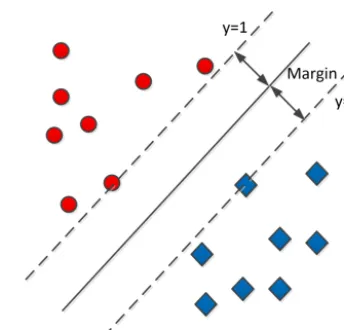
Figure 5. Decision boundary of support vector machine.

is the probability of observing a certain class before the fea-ture of unknown samplex is taken into account. The class-conditional probability is learned from the training samples. It is usually modeled using Gaussian functions, as defined in Eq. (6). For simplicity, we can assume that all the classes have the same prior probabilities. It is also possible to set the prior probabilities according to the frequency of appearance of each class in the training data set.

P (ωk|x)=

P (ωk)P (x|ωk)

P (x) (5)

P (x|ωk)=

1 (2π )p/2_|₆

k|1/2

e−12(x−µk)6k(x−µk)T ₍₆₎ To model class-conditional probabilities as Gaussians, we need to estimate the parameters of the Gaussians from the training data. Regularization techniques help reduce variance without adding too much model bias when estimating the pa-rameters for high-dimensional data (Cheng et al., 2010). In eigenvalue decomposition regularized discriminant analysis (EDRDA) (Bensmail and Celeux, 1996), the covariance ma-trixP

k for thekth class is re-parameterized in terms of its

eigenvalue decomposition P

k=αkDkAkDT_k, where αk=

P_k

1/p

andDk is the matrix of eigenvectors of P_k. The

matrix Ak is a diagonal matrix such that|Ak| =1 with the

normalized eigenvalues ofP

k on the diagonal in a

decreas-ing order. By allowdecreas-ing each of the parametersαk,Ak, Dkto

be either the same or different among different classes, eight discriminant models can be obtained. Furthermore, six more models are obtained by modeling the covariance matrix as a diagonal matrix or a scalar multiple of the identity matrix. More specifically,P

k=αkBk leads to four more less

com-plex models, where Bk is a diagonal matrix with |Bk| =1.

The models requiring the smallest numbers of parameters are to assume spherical shapes, i.e., Ak is an identity

(6)

Figure 6. Example of correcting a stratus block as cumulus.

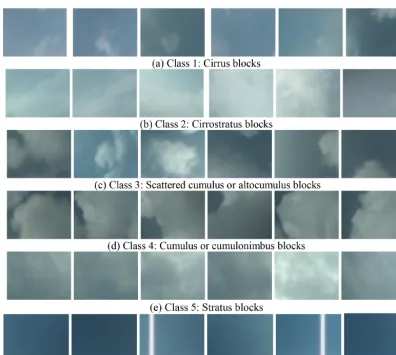
Figure 7. Example of training blocks.

models, there are nine models whose maximum likelihood (ML) estimation of the covariance matrix can be computed in closed form. For other models, the ML estimation needs to be computed through an iterative procedure. To acceler-ate the model selection process, this work only considers the nine EDRDA models that have closed-form solutions for ML parameter estimation.

2.5.2 Support vector machine

(7)

(e) Class 5: Stratus blocks 290

291

(f) Class 6: Clear sky 292

Figure 7. Example of training blocks 293

294

295

(a) (b) 296

Figure 8. Examples of images with two ground truth labels 297

298

To select the proper threshold

Thr

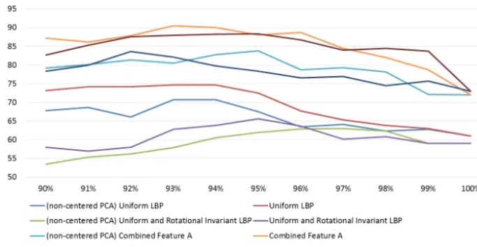
_PCA

for dimension reduction, we plot the accuracy using different

Thr

_PCA

in

299

Figure 9. We use the 1800 blocks with ground truth labels and perform 10-fold cross validation (CV) when

300

conducting this experiment. Note that the CV accuracy in Figure 9 is based on the classification result of

reduction. For combined feature A and combined feature B, the advantage of applying PCA is more obvious

308

since the dimensionality is higher. The statistical feature vector has only 12 dimensions. Therefore, there is no

309

need to apply PCA on the statistical feature vector.

310

311

Figure 8. Examples of images with two ground truth labels.

the trained classifier with the large margins. The reason is that unseen testing samples may fall within the large margin and hopefully will still be correctly classified. To determine the hyper-plane that results in maximized margin, the sup-port vector machine solves the quadratic programming op-timization problem. Furthermore, to effectively handle non-linear separable data in the real world, the concept of soft margin and the usage of kernel functions are applied in the SVM. The details can be found in the work of Cristianini and Shawe-Taylor (2000). In this work, we apply SVM with radial basis functions as kernel functions.

2.6 Post-processing

In the process of block division, the important information of global cloud-cover percentage is inevitably lost. There-fore, we examine the classification result of each block in the post-processing step. Connected component analysis is per-formed on the cloud detection results. If a block is classified as stratus but the size of the cloud component is lower than the threshold, the label of the block is revised to cumulus. An example is shown in Fig. 6. The cloud detection result with connected component labeling is shown in Fig. 6b. Differ-ent connected componDiffer-ents are illustrated in differDiffer-ent colors. The numbers on each component denote the number of pix-els in the component. We can observe that three blocks are re-labeled as cumulus. In our experiments, the threshold for revising the classification result is 12 000 pixels.

The subsequent application modules can utilize the classi-fication result of each individual block with the knowledge of the location of the block. The classification results of all the blocks in an image can also be gathered to obtain a summa-rized label for the entire image. A simple way to summarize the labels in an image is to perform voting. From the classi-fication results in Fig. 6, we have the knowledge that there are more votes for class 3 than other classes in this all-sky image.

3 Experiments and discussions

In this section, we report experimental results and discuss the performance of the proposed block-based cloud classifica-tion framework. For training purposes, we select 1800 blocks from the images and manually label the ground truth of these blocks. Selected training blocks for the six classes are shown in Fig. 7. Note that the block size used in our experiments is 60×80 pixels. We manually classified the ground truth of 3000 images in the data set in order to calculate the summa-rized classification accuracy for whole images. Since there are mixed cloud conditions in many images, each image can be associated with at most two ground truth labels. For a mixed cloud type image, the voting result is considered cor-rect if the classified label matches any of the two ground truth labels. Figure 8 displays some examples of images that are associated with two ground truth labels. Figure 8a is labeled as both class 2 and class 4. Figure 8b is labeled as both class 1 and class 3. Due to the privacy issue of the data provider, we use a mask on the image to eliminate the surrounding build-ings. The experiment data set includes all-sky images from 08:30 to 15:30 (UTC+8 h). Therefore, the data set does not include the cases when the sun is close to the mask limits.

(8)

Figure 9. Selection of the threshold ThrPCAfor dimension reduction.

Figure 10. Classification accuracy on blocks using different feature and classifier combinations.

dimensionality reduction. For combined feature A and com-bined feature B, the advantage of applying PCA is more obvi-ous since the dimensionality is higher. The statistical feature vector has only 12 dimensions. Therefore, there is no need to apply PCA on the statistical feature vector.

To compare the effect of various features and classifiers, Fig. 10 shows the 10-fold cross-validated classification ac-curacy on the 1800 blocks with ground truth labels using different features and classifiers. Compared with the statis-tical features and k-NN classifier used in the work by Heinle et al. (2010), the proposed combined features with Bayesian classifier or SVM demonstrate higher classification rates. It is clear that local texture feature alone does not perform bet-ter than statistical features. However, when combined with statistical features, additional information provided by dis-tribution of local texture features can significantly improve the classification accuracy. We can observe that combined feature A slightly outperforms combined feature B when us-ing the Bayesian classifier and SVM. Although intuitively we think that features with rotation invariant characteristics

should be preferable for cloud classification, combined fea-ture A performs slightly better in practice. It might be due to the small dimensionality of combined feature B. Overall, the method using combined feature A and the Bayesian clas-sifier with regularized discriminant analysis has the highest cross-validated classification accuracy in our experiments. Figure 11 displays selected classification results using com-bined feature A and the Bayesian classifier with regularized discriminant analysis. Although there are inevitably some misclassified blocks, most blocks are correctly classified in Fig. 11. Note that classification labels are not displayed on incomplete blocks and the block where the sun resides in Fig. 11.

(9)

319

320

Figure 11.Selected classification results. 321

322

To compare the effect of various features and classifiers, Figure 10 shows the 10-fold cross validated 323

classification accuracy on the 1800 blocks with ground truth labels using different features and classifiers. 324

Compared with the statistical features and k-NN classifier used in the work by Heinle et al. (Heinle et al., 325

2010), the proposed combined features with Bayesian classifier or SVM demonstrate higher classification 326

rates. It is clear that local texture feature alone does not perform better than statistical features. However, 327

when combined with statistical features, additional information provided by distribution of local texture 328

features can significantly improve the classification accuracy. We can observe that combined feature A 329

slightly outperforms combined feature B when using Bayesian Classifier and SVM. Although intuitively we 330

think that features with rotation invariant characteristics should be preferable for cloud classification, 331

combined feature A performs slightly better in practice. It might be due to the small dimensionality of 332

Figure 11. Selected classification results.

Figure 12. Comparison of whole-image classification and block-based classification with voting scheme.

block-based classification is that the classification result of each individual block with the knowledge of the block loca-tion can be utilized by subsequent applicaloca-tion modules.

We perform an experiment to compare the proposed method with the method of Kazantzidis et al. (2012). The method of Kazantzidis et al. outperforms the proposed work with the concept of subclass division. In addition to com-paring the method proposed by Kazantzidis et al., we also apply the concept of subclass division in our framework in the experiment. Since we have the information of the source image from which a training or testing block is selected, we could obtain the information needed to separate a block into subclasses. The subclasses are divided according to the so-lar zenith angle, global cloud coverage of the all-sky image,

Figure 13. Comparison of classification results of different methods on the effect of subclass division and block voting.

(10)

block voting, and subclass division would yield the best re-sult.

4 Conclusions

Cloud classification is an important task for improving short-term solar irradiance prediction since different types of clouds have different effects on the change of solar irradi-ance. In this work, an automatic cloud-classification method for all-sky images is proposed. The classification is per-formed based on fixed-size blocks in the all-sky images. In addition to the statistical features in the literature, we com-bine the histogram of local texture patterns in the feature vec-tor. With more discriminate features provided by local tex-ture patterns, the proposed combined featex-ture can improve the classification accuracy. Replacing k-NN classifier with more sophisticated supervised learning methods can further enhance the recognition results. Bayesian classifier with reg-ularized discriminant analysis outperforms other classifiers on this data set in our experiments. This work also com-pares the classification accuracy with and without the vot-ing scheme. With block-based classification and the votvot-ing scheme, the classification results on images with mixed cloud type conditions were shown to be better. Although the global cloud coverage feature is lost in the block-based feature ex-traction process, the global cloud coverage information can still be used to divide the data set into subclasses, as sug-gested in the work of Kazantzidis et al., to improve the clas-sification accuracy of the proposed framework. For future work in component-based cloud classification, each detected connected component of cloud can be classified separately. In this way, the situation of mixed cloud types could be analyzed with even better precision and the information of the cloud coverage can be preserved. However, the perfor-mance of component-based classification would be highly dependent on the cloud detection accuracy. Therefore, cur-rent cloud detection methods need to be improved in order to lead to satisfactory component-based classification results. In addition to component-based cloud classification, another potential future work is to integrate the proposed cloud clas-sification method in a short-term irradiance prediction sys-tem to obtain more accurate prediction results.

Acknowledgements. This work was supported in part by the

Ministry of Science and Technology of Taiwan.

Edited by: V. Amiridis

References

Bensmail, H. and Celeux, G.: Regularized Gaussian discriminant analysis through eigenvalue decomposition, J. Am. Stat. Assoc., 91, 1743–1748, 1996.

Cadima, J. and Jolliffe, I.: On relationships between uncentered and column-centered principal component analysis, Pak. J. Statist., 25, 473–503, 2009.

Calbo, J. and Sabburg, J.: Feature extraction from whole-sky ground-based images for cloud-type recognition, J. Atmos. Ocean. Tech., 25, 3–14, 2008.

Cheng, H. Y., Yu, C. C., Tseng, C. C., Fan, K. C., Hwang, J. N., and Jeng, B. S.: Environment classification and hierarchical lane detection for structured and unstructured roads, IET Computer Vision, 4, 37–49, 2010.

Cristianini, N. and Shawe-Taylor, J.: An introduction to support vector machines and other kernel-based learning methods, Cam-bridge University Press, CamCam-bridge, England, 2000.

Duda, R. O., Hart, P. E., and Stork, D. G.: Pattern classification, John Wiley & Sons, New York City, NY, USA, 2nd edn, 2001. Fu, C. L. and Cheng, H. Y.: Predicting solar irradiance with all-sky

image features via regression, Solar Energy, 97, 537–550, 2013. Haralick, R. M., Shanmugam, K., and Dinstein, I.: Textural features for image classification, IEEE Transactions on Systems, Man and Cybernetics, 3, 610–621, 1973.

Heinle, A., Macke, A., and Srivastav, A.: Automatic cloud classi-fication of whole sky images, Atmos. Meas. Tech., 3, 557–567, doi:10.5194/amt-3-557-2010, 2010.

Kassianov, E., Long, C. N., and Ovtchinnikov, M.: Cloud sky cover versus cloud fraction: Whole-sky simulations and observations, J. Appl. Meteor., 44, 86–98, 2005.

Kazantzidis, A., Tzoumanikas, P., and Bais, A. F.: Fotopoulos S, Economou G, Cloud detection and classification with the use of whole-sky ground-based images, Atmos. Res., 113, 80–88, 2012. Kubota, M., Nagatsuma, T., and Murayama, Y.: Evening corotat-ing patches: A new type of aurora observed by high sensitiv-ity all-sky cameras in Alaska, Geophys. Res. Lett., 30, 1612, doi:10.1029/2002GL016652, 2003.

Li, Z., Cribb, M. C., Chang, F. L., and Trishchenko, A. P.: Valida-tion of MODIS-retrieved cloud fracValida-tions using whole sky imager measurements at the three ARM sites, Proc. 14th ARMScience Team Meeting, Albuquerque, NM, Atmospheric Radiation Mea-surement Program, 6, 2–6, 2004.

Long, C. N., Sabburg, J., Calbó, J., and Pagès, D.: Retrieving cloud characteristics from ground-based daytime color all-sky images, J. Atmos. Ocean. Tech., 23, 633–652, 2006.

Martínez-Chico, M., Batlles, F. J., and Bosch, J. L.: Cloud classi-fication in a mediterranean location using radiation data and sky images, Energy, 36, 4055–4062, 2011.

Pfister, G., McKenzie, R. L., Liley, J. B., Thomas, A., Forgan, B. W., and Long, C. N.: Cloud coverage based on all-sky imaging and its impact on surface solar irradiance, J. Appl. Meteorol., 42, 1421–1434, 2003.

Singh, M. and Glennen, M.: Automated ground-based cloud recog-nition, Pattern Anal. Appl., 8, 258–271, 2005.