www.ocean-sci.net/4/239/2008/
© Author(s) 2008. This work is distributed under the Creative Commons Attribution 3.0 License.
Ocean Science
Improving the parameterisation of horizontal density gradient in
one-dimensional water column models for estuarine circulation
S. Blaise1and E. Deleersnijder2
1Universit´e catholique de Louvain, Unit´e de G´enie Civil et Environnemental, Louvain-la-Neuve, Belgium
2Universit´e catholique de Louvain, Centre for Systems Engineering and Applied Mechanics, Louvain-la-Neuve, Belgium
Abstract. A new parameterisation of horizontal density gra-dient for a one-dimensional water column estuarine model, inspired by the first-order finite-difference upwind scheme, is presented. This parameterisation prevents stratification from growing indefinitely, a deficiency usually referred to as “run-away stratification”. It is seen that, using this upwind-like pa-rameterisation, the salinity must remain comprised between upper and lower bounds set a priori and that any initial over-or under-shooting is progressively eliminated. Simulations of idealised and realistic estuarine regimes indicate that the new parameterisation lead to results that are devoid of the runaway stratification phenomenon, as opposed to previously used models.
1 Introduction
Estuaries and their regions of freshwater influence (ROFIs) have been studied for a long time. They exhibit strong gradi-ents of several variables: salinity, temperature, plankton and nutrient concentrations can vary over a wide range of values, strongly impacting physical and biological processes. For in-stance, complex dynamics, influenced by tides and input of freshwater from rivers, have a strong influence on the growth of phytoplankton (Lucas et al., 1998, 1999).
This work focuses on estuarine dynamics, especially on the evolution of stratification. The latter is a key player in vertical mixing, which influences directly the vertical fluxes of heat, salt, momentum and nutrients (Simpson et al., 1990). Many studies were devoted to the evolution of stratification in estuaries. They firstly described in situ observations gath-ered from field surveys (Sharples and Simpson, 1993; Stacey and Monismith, 1999), showing that the dynamics is mainly
Correspondence to: S. Blaise ([email protected])
driven by the tidal flow associated with a density driven cir-culation generated by an input of freshwater from rivers. This was reproduced in laboratory experiments by Linden and Simpson (1986, 1988), who focused on the mechanisms influencing stratification. These mechanisms were described in detail by Simpson et al. (1990). Several models were ap-plied to simulate and understand the evolution of stratifica-tion in estuaries. Linear prescriptive models were first used (Simpson et al., 1991; Nunes Vaz and Simpson, 1994; Scott, 2004). Then, several authors turned to one-dimensional wa-ter column non linear models (Monismith et al., 1996; Moni-smith and Fong, 1996; Nunes Vaz and Simpson, 1994; Lucas et al., 1998). Recently, three-dimensional models were used to simulate estuarine flows (Burchard and Baumert, 1998; Hetland and Geyer, 2004; Warner et al., 2005).
One-dimensional non linear models can be very useful to understand and predict the evolution of stratification in an estuary. They are light and simple to build. They require a minimal amount of data and parameters. Furthermore, they generate simple results, which permits to easily understand the key processes and quickly establish diagnoses. However, one common failure of these models is the generation of run-away stratification: when the tidal amplitude is low, strati-fication tends to grow without bound due to an inadequate parameterisation of horizontal density gradient (Nunes Vaz and Simpson, 1994; Monismith et al., 1996; Warner et al., 2005). This paper shows that simple analytical developments can lead to a new version of the model which keeps stratifi-cation under control. It is also seen that, in the long run, the model is insensitive to an unrealistic initial stratification.
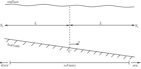
Fig. 1. Physical setting: the stratification is to be simulated in the water column located at pointC. The latter is located in a region of high salinity gradient. Its order of magnitude is(Ss−Sr)/2L,
whereSsandSrdenote the downstream and the upstream salinity,
respectively.
of stratification in estuaries (Nunes Vaz and Simpson, 1994). This turbulence closure was recently implemented using the finite-element method for one-dimensional (Hanert et al., 2006) and three-dimensional (Blaise et al., 2007) models.
The physical setting is described in Sect. 2. Then, in Sect. 3, the model is presented. Two parameterisations of horizontal density gradient, the classical one and a new one, are introduced in Sect. 4 and it is seen rigorously that the new approach prevents stratification from running away. This is illustrated by numerical results in Sect. 5. Section 6 exam-ines the sensitivity of the model to the initial stratification. Finally, conclusions are drawn in Sect. 7.
2 Physical setting
We will study the stratification in an estuary, which is gen-erated by the front between freshwater and salty seawater. This front is of a crucial importance for the dynamics of the estuary, notably for the vertical density gradient. Therefore, we will consider a water column located atC in Fig. 1, at a distanceLto the sea limit. We assume that the salinity at a distanceLupstream ofC is of the order ofSr and that the
salinity at the sea limit is of the order ofSs. We also assume
thatSr andSs are constants satisfying the following
condi-tion:
Sr<Ss. (1)
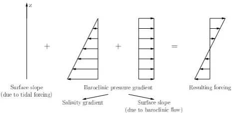
In such a configuration, the water velocity is mainly caused by two processes (Simpson et al., 1990):
– The presence of freshwater originating from the river creates a density front with the salty seawater (Fig. 2a). This front induces a circulation, with light freshwater going towards the sea at the surface, and dense water going towards the river near the bottom. Due to the tom friction, this circulation is reduced near the sea bot-tom.
(a)
(b)
Fig. 2. Circulation induced (a) by the freshwater input generating a front with the dense seawater and (b) by tides (here at falling tide), as described by Simpson et al. (1990).
bottom velocities during rising tides than during falling tides, which has the effect of increasing the stratifica-tion.
The combination of these processes can generate different flow regimes. If the tides are dominant, the SIPS regime prevails. When the effect of the horizontal density gradi-ent becomes important compared to the tidal effect, the tidal mixing is not sufficient to annihilate the stratification; this stratification strengthens during each tidal cycle, inducing a persistent stratification regime (Lucas et al., 1998). The pres-ence of different non-synchronous tidal components, by gen-erating an alternation of spring/neap tides, can lead to a suc-cession of SIPS and permanent stratification periods (Simp-son et al., 1990; Sharples and Simp(Simp-son, 1993; Nunes Vaz and Simpson, 1994; Monismith et al., 1996).
3 Model description
The model used herein is based on that of Lucas et al. (1998) and Monismith et al. (1996). For the flow under study, the impact on density of temperature variations is negligi-ble compared with those of salinity. Therefore, density is assumed to be a function of salinity only and the following equations will be expressed in terms of salinity. As in Lucas et al. (1998) and Monismith et al. (1996), a linear equation of state is adopted:
ρ=ρ0(1+β(S−S0)) , (2)
where ρ and S are the density and the salinity, whose reference values are denoted ρ0 and S0, respectively;
β=7.6·10−4 psu−1 is the salinity expansion coefficient, which is assumed to be constant.
Ifxis the horizontal coordinate increasing toward the sea, the along-estuary horizontal velocity u(t, z) at location C
obeys the following momentum equation:
∂u ∂t = −g
∂η
∂x −gβ
∂S ∂x
−z+γH
2
+ ∂
∂z
ν∂u ∂z
, (3)
whereg,η,zandHare the gravitational acceleration, the sea surface elevation, the vertical coordinate pointing upwards with its origin at the sea surface and the constant water depth, respectively. The effect of Earth rotation is neglected. The surface stress and bottom velocity are equal to zero. The tur-bulent viscosityν is calculated by means of the Mellor and Yamada level 2.5 turbulence closure (Mellor and Yamada, 1974, 1982) implemented in its quasi-equilibrium version (Galperin et al., 1988; Deleersnijder and Luyten, 1994). The surface slope due to the barotropic tides can be represented as
−g∂η
∂x =
X
i
Ui,max 2π
Ti
cos
2π Ti
t
(4)
in whichTi is the tide period andUi,maxthe maximum ve-locity for thei-th tidal component. The baroclinic pressure gradient can be divided into two contributions (Lucas et al., 1998; Monismith et al., 1996): a term derived from the hori-zontal salinity gradient,gβ∂S∂xz, and a term derived from the surface slope generated by the baroclinic flow,−gβ∂S∂xγH2. The dimensionless coefficientγ is to be tuned in such a way that the residual transport is zero, i.e. the average over a tidal cycle of the depth-integrated velocity vanishes. Practically,
γ is found iteratively to minimize this velocity (Lucas et al., 1998). It is possible to impose a prescribed mean velocity, and in this way take into account the effect of residual run-off from the river (Burchard, 1999), but this was not done in the present paper.
The salinitySobeys the equation
∂S ∂t = −u
∂S
∂x +
∂ ∂z
λ∂S
∂z
, (5)
where the eddy diffusivityλis obtained from the same tur-bulence closure model as the eddy viscosity. The surface and bottom salinity fluxes are prescribed to be zero:
λ∂S
∂z
z=−H,0
=0. (6)
4 Parameterisation of the horizontal salinity gradient
In the previous governing equations, most authors (Nunes Vaz and Simpson, 1994; Lucas et al., 1998; Monismith et al., 1996; Monismith and Fong, 1996) assumed the horizontal salinity gradient to be a constant that was evaluated as fol-lows:
∂S
∂x=τ, (7)
where τ=Ss−Sr
2L . In some situations (e.g. for some
ide-alised studies or when it is in accordance with observations), it is a good choice to prescribe the salinity gradient as a constant. However, this parameterisation has been identi-fied as the cause of the so-called “runaway stratification”, a phenomenon in which stratification increases indefinitely (Warner et al., 2005). The salinity reaches values that are no longer comprised in the interval[Sr, Ss], which is
unac-ceptable. By annihilating vertical mixing, this overestimated stratification corrupts the computation of the evolution of ve-locity and water properties.
Fig. 3. Vertical profiles of the tidally-averaged forcing terms ap-pearing in the momentum Eq. (3). The resulting forcing varies lin-early with depth.
salinity gradient in (5) will inevitably lead to a constantly increasing stratification if mixing is not taken into account. Indeed, at falling tide, the advection of freshwater will de-crease with depth whereas, at rising tide, the advection of seawater will increase with depth, causing stratification to grow indefinitely. The turbulent mixing can counterbalance this phenomenon and stabilize the stratification, especially at the end of rising tide when its effect surpasses the effect of advection. At falling tide, the mixing is intense due to the low or unstable stratification, contributing to a non stratified water column. However, if turbulent mixing is not sufficient, the water column will stratify indefinitely.
The apparition of “runaway stratification” can be avoided by using an alternative parameterisation of the horizontal salinity gradient, inspired by the first-order upwind differ-ence scheme:
∂S
∂x =
(S−S r
L ifu≥0,
Ss−S
L ifu <0.
(8)
By introducingu+andu−the positive and negative parts of the longitudinal velocity,
u±=u± |u|
2 , (9)
and by using relation (8), we can rewrite Eq. (5) as
∂S ∂t = −u
+S−Sr
L −
u−
S−Ss
L +
∂ ∂z
λ∂S
∂z
. (10)
If the velocity is directed toward the sea (u>0), the first term in the right-hand side of (10) relaxes the salinity to its river valueSr, the relaxation timescale beingL/u+. On the other
hand, when the velocity is directed toward the river, the salin-ity is relaxed towardSs with a relaxation timescale equal to
L/|u−|.
It is interesting to notice that resorting to this new parame-terisation is equivalent to add to the classical formulation (7)
a horizontal diffusion term. Indeed, with the parameterisa-tion suggested herein, the horizontal salinity advecparameterisa-tion may be rewritten as (E. Hanert, personal communication, 2008) −u∂S
∂x = −u Ss−Sr
2L +
|u|L
2
Ss −2S+Sr
L2 . (11)
Clearly, the last term in the equation above may be viewed as the discrete form of the harmonic diffusion operator, the associated diffusivity being|u|L/2.
The interpretation of the role of the first two terms in the right-hand side of salinity Eq. (10) suggests that, whatever the horizontal velocity, the salinity should tend to be com-prised in the interval [Sr, Ss]. In fact, this can be
demon-strated rigorously. For an arbitrary large value oft(t→∞), the salinity must obey the following inequalities:
Sr≤S(t, z)≤Ss, (12)
implying that stratification cannot grow out of control. We first define the overshooting of the salinity by
δ+=max [0, S(t, z)−Ss] (13)
So, the overshooting is a positive variable that is equal to
S(t, z)−Ss if the salinity is greater than its sea valueSs, and
is equal to zero otherwise. Multiplying Eq. (10) by the over-shooting and integrating over the height of the water column yields:
1 2
d dt
Z 0
−H
δ+2dz=
− Z 0
−H
u+S−Sr
L +
u−
S−Ss
L
δ+dz
− Z 0
−H
λ
∂δ+ ∂z
2
dz. (14) The manipulations leading to this equation are not trivial, but they are of the same type as those of Appendix C of Deleer-snijder et al. (2001). All of the terms in the right-hand side of (14) are negative unless the overshooting is zero at every point of the water column. Thus, the quadratic measure of the overshooting tends to zero as time increases, implying that
lim
t→∞δ
+=
0. (15)
Combining relations (13) and (15) leads to
S(t, z)≤Ssfort→ ∞. (16)
A similar analysis can be performed for the undershooting
δ−=max [0, Sr−S(t, z)], eventually leading to S(t, z)≥Sr
fort→∞. Hence, (12) holds valid. QED.
0 1 2 3 4 5 6 7 8 9 10 −0.5
0 0.5 1 1.5
Sbottom
− S
surface
[psu]
0 1 2 3 4 5 6 7 8 9 10 15.5
16 16.5 17 17.5 18 18.5
S [psu]
0 1 2 3 4 5 6 7 8 9 10 −1
−0.5 0 0.5 1
umean
[m/s]
Tidal cycles
old parameterisation (7) new parameterisation (8)
Fig. 4. Simulation of a Strain-Induced Periodic Stratification (SIPS) regime: results obtained using the old (7) (dashed curves) and the new (8) (solid curves) parameterisations of the hori-zontal salinity gradient. The tidal forcing is characterised by
U0,max=1 m/s andT0=12 h. The longitudinal salinity gradient is set toτ=0.25 psu/km. The bounds of salinity are set toSr=0 psu
andSs=35 psu. Upper panel: Evolution of the stratification
(differ-ence between bottom salinity and surface salinity). Middle panel: Minimum and maximum values of salinity over the water column. Lower panel: Evolution of the depth-averaged velocity. The latter is similar for both parameterisations.
5 Model results
To illustrate the advantages of the parameterisation designed above, we will simulate the situations described in Sect. 2. All of the simulations are achieved using a time-step of 60 seconds. The one-dimensional vertical mesh contains 30 nodes. The main physical parameters are similar to those of Nunes Vaz and Simpson (1994). The water column depth is 15 m, and the values ofSr andSs are respectively 0 psu
and 35 psu.
We first consider a SIPS regime similar to that of Nunes Vaz and Simpson (1994). There is only one tidal com-ponent with a magnitude of U0,max=1 m/s and a period of T0=12 h. The longitudinal constant salinity gradient
τ is set to 0.25 psu/km. Figure 4 shows that the SIPS regime is quickly established, with an alternation of strati-fied/unstratified phases. The tidal mixing at the end of the
0 2 4 6 8 10 12 14 16 18 20 0
10 20 30 40 50
Sbottom
− S
surface
[psu]
0 2 4 6 8 10 12 14 16 18 20 −50
0 50
S [psu]
0 2 4 6 8 10 12 14 16 18 20 −0.4
−0.2 0 0.2 0.4
umean
[m/s]
Tidal cycles
old parameterisation (7) new parameterisation (8)
Fig. 5. Simulation of a persistent stratification regime: results ob-tained using the old (7) (dashed curves) and the new (8) (solid curves) parameterisations of the horizontal salinity gradient. The tidal forcing is characterised byU0,max=0.5 m/s andT0=12 h. The longitudinal salinity gradient is set toτ=0.3 psu/km. The bounds of salinity are set toSr=0 psu andSs=35 psu. Upper panel:
Evo-lution of the stratification (difference between bottom salinity and surface salinity). Middle panel: Minimum and maximum values of salinity over the water column. Lower panel: Evolution of the depth-averaged velocity. The latter is similar for both parameterisa-tions.
falling tide is sufficient to annihilate stratification. The latter is very similar using both parameterisations of salinity gra-dient. However, the constant parameterisation (7) leads to higher peaks of stratification while the latter is limited us-ing the new parameterisation (8). These smaller peaks can be explained by the horizontal diffusion added to the model (11) when we use the new parameterisation of salinity gradi-ent. The mean velocity remains rather insensitive to the used parameterisation.
0 10 20 30 40 50 60 −20
−10 0 10 20 30 40
Sbottom
− S
surface
[psu]
0 10 20 30 40 50 60
−30 −20 −10 0 10 20
S [psu]
0 10 20 30 40 50 60
−1 −0.5 0 0.5 1
umean
[m/s]
Tidal cycles
old parameterisation (7) new parameterisation (8)
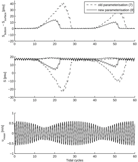
Fig. 6. Simulation of the circulation induced by a succession of spring/neap tides: results obtained using the old (7) (dashed curves) and the new (8) (solid curves) parameterisations of the horizontal salinity gradient. The tidal forcing is characterised by
U0,max=0.8 m/s,T0=12.42 h,U1,max=0.46·U0,maxandT1=12 h. The longitudinal salinity gradient is set to τ=0.25 psu/km. The bounds of salinity are set toSr=0 psu andSs=35 psu. Upper panel:
Evolution of the stratification (difference between bottom salinity and surface salinity). Middle panel: Minimum and maximum val-ues of salinity over the water column. Lower panel: Evolution of the depth-averaged velocity. The latter is similar for both parame-terisations.
displayed on Fig. 5. Using the classical parameterisation of the horizontal salinity gradient, the stratification grows out of control to unrealistic values exceeding the imposed bounds, which is the deficiency known as “runaway stratification”. As demonstrated in Sect. 4, the stratification remains within the imposed limits when we use the new parameterisation. The slight oscillations show that, even when the stratifica-tion is high, it is still influenced by tide. While the classical parameterisation (7) gives useless results, the new parame-terisation (8) gives qualitatively realistic results for a large number of tidal cycles.
The spring/neap cycles are now simulated by taking into account two tidal components. The first one has an amplitude of U0,max=0.8 m/s and a period of T0=12.42 h; while the second component has an amplitude ofU1,max=0.46·U0,max and a period of T1=12 h (Nunes Vaz and Simpson, 1994).
Using this combination of tidal components, we generate an alternation of spring and neap tides (Fig. 6). We set the longitudinal constant salinity gradient to the value of
τ=0.25 psu/km. It is shown on Fig. 6 that both parameterisa-tions represent a spring-neap cycle of stratification. During neap tides, the stratification grows until the tidal amplitude increases at spring tides. Then, the stratification weakens and comes back to a SIPS regime. However, the classical parameterisation leads to unrealistic peaks of stratification, with salinity exceeding the limits imposed by the river and sea salinities. This is a common issue when using expression (7) (i.e. Nunes Vaz and Simpson (1994) in which the differ-ence between bottom and surface density grows during neaps as far as 180 kg/m3). This problem does not occur when the new parameterisation is resorted to.
In the last experiment, we simulate a spring-neap cy-cles regime giving rise to runaway stratification. To this aim, the tidal amplitude is decreased toU0,max=0.7 m/s and
U1,max=0.46·U0,max, while the longitudinal constant salin-ity gradient is increased toτ=0.3 psu/km. Figure 7 shows that the classical parameterisation of the horizontal salinity gradient term leads to a stratification which increases un-boundedly and then cannot come back to the SIPS regime. During successive tidal cycles, the stratification strengthen to excessively large values. The new parameterisation, by lim-iting the peak of stratification to acceptable values, permits to come back to the SIPS regime during spring tides which is believed to be consistent with observation (Simpson et al., 1990; Sharples and Simpson, 1993).
6 Discussion
0 10 20 30 40 50 60 0
20 40 60 80 100
Sbottom
− S
surface
[psu]
0 10 20 30 40 50 60
−100 −50 0 50
S [psu]
0 10 20 30 40 50 60
−1 −0.5 0 0.5 1
umean
[m/s]
Tidal cycles
old parameterisation (7) new parameterisation (8)
Fig. 7. Simulation of the circulation induced by a of succes-sion spring/neap tides: results obtained using the old (7) (dashed curves) and the new (8) (solid curves) parameterisations of the horizontal salinity gradient. The tidal forcing is characterised by
U0,max=0.7 m/s,T0=12.42 h,U1,max=0.46·U0,maxandT1=12 h. The longitudinal salinity gradient is set to τ=0.3 psu/km. The bounds of salinity are set toSr=0 psu andSs=35 psu. Upper panel:
Evolution of the stratification (difference between bottom salinity and surface salinity). Middle panel: Minimum and maximum val-ues of salinity over the water column. Lower panel: Evolution of the depth-averaged velocity. The latter is similar for both parame-terisations.
By slightly modifying the equations, the present model could also be applied to the simulation of the tidal strain-ing in a Region of Freshwater Influence (ROFI), for which the stratification induced by a gradient of density is also a key process (Visser et al., 1994). The new parameterisation of the salinity gradient should be able to avoid the generation of runaway stratification in a ROFI model, for which this nu-merical complication can also occur.
7 Conclusions
Using simple mathematical developments, a new expression of the horizontal density gradient was developed in order to avoid the phenomenon known as “runaway stratification”. This method allows for the simulation of rather realistic flows
(a)
0 5 10 15 20
0 20 40 60 80 100 120
S bottom
− S
surface
[psu]
Tidal cycles
old parameterisation (7) new parameterisation (8)
(b)
0 5 10 15 20
0 20 40 60 80 100 120
S bottom
− S
surface
[psu]
Tidal cycles
old parameterisation (7) new parameterisation (8)
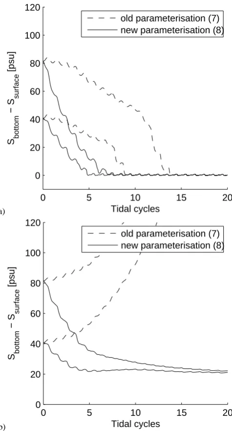
Fig. 8. Sensitivity to the initial stratification: evolution of the strati-fication (difference between bottom salinity and surface salinity) for the different parameterisations of the horizontal salinity gradient, in the case of a SIPS regime (a) and persistent stratification (b). Two simulation results are showed for both regimes, with initial differ-ences between bottom salinity and surface salinity set to 40 psu and 80 psu.
to derive a priori upper or lower bounds of their solution. This technique is inspired by Lewandowski (1997). To the best of our knowledge, it has been used in a small num-ber of oceanographic studies only (Deleersnijder et al., 2001; Legrand et al., 2006; Gourgue et al., 2007).
Acknowledgements. S´ebastien Blaise is a Research fellow with the
Belgian Fund for Research in Industry and Agriculture (FRIA). Eric Deleersnijder is a Research associate with the Belgian National Fund for Scientific Research (FNRS). The present study was carried out within the scope of the project “A second-generation model of the ocean system”, which is funded by the Communaut´e Franc¸aise
de Belgique, as Actions de Recherche Concert´ees, under contract
ARC 04/09-316 and the project “Tracing and Integrated Modelling of Natural and Anthropogenic Effects on Hydrosystems” (TIMO-THY), an Interuniversity Attraction Pole (IAP6.13) funded by the
Belgian Federal Science Policy Office (BELSPO). This work is a
contribution to the development of SLIM, the Second-generation Louvain-la-Neuve Ice-ocean Model (http://www.climate.be/SLIM).
Edited by: E. J. M. Delhez
References
Blaise, S., Deleersnijder, E., White, L., and Remacle, J.-F.: Influ-ence of the turbulInflu-ence closure scheme on the finite-element sim-ulation of the upwelling in the wake of a shallow-water island, Cont. Shelf Res., 27, 2329–2345, 2007.
Burchard, H.: Recalculation of surface slopes as forcing for numer-ical water column models and tidal flow, Appl. Math. Mod., 23, 737–755, 1999.
Burchard, H. and Baumert, H.: The formation of estuarine turbidity maxima due to density effects in the salt wedge. A hydrodynamic process study, J. Phys. Oceanogr., 28, 309–321, 1998.
Deleersnijder, E. and Luyten, P.: On the practical advantages of the quasi-equilibrium version of the Mellor and Yamada level 2.5 turbulence closure applied to marine modelling, App. Math. Mod., 18, 281–287, 1994.
Deleersnijder, E., Campin, J.-M., and Delhez, E. J. M.: The concept of age in marine modelling I. Theory and preliminary model re-sults, J. Mar. Sys., 28, 229–267, 2001.
Galperin, B., Kantha, L., Hassid, S., and Rosati, A.: A quasi-equilibrium turbulent energy model for geophysical flows, J. At-mos. Sci., 45, 55–62, 1988.
Gourgue, O., Deleersnijder, E., and White, L.: Toward a generic method for studying water renewal, with application to the epil-imnion of Lake Tanganyika, Estuarine, Coastal and Shelf Sci-ence, 74, 764–776, 2007.
Hanert, E., Deleersnijder, E., and Legat, V.: An adaptative finite element water column model using the Mellor-Yamada level 2.5 turbulence closure scheme, Ocean Model., 12, 205–223, 2006. Hanert, E., Deleersnijder, E., Blaise, S., and Remacle, J.-F.:
Cap-turing the bottom boundary layer in finite element ocean models, Ocean Model., 17, 153–162, 2007.
Hetland, R. D. and Geyer, W. R.: An idealized study of the structure of long, partially mixed estuaries, J. Phys. Oceanogr., 34, 2677– 2691, 2004.
Jay, D. A. and Musiak, J. D.: Particle trapping in estuarine tidal flows, J. Geophys. Res., 99, 445–461, 1994.
Legrand, S., Deleersnijder, E., Hanert, E., Legat, V., and Wolan-ski, E.: High-resolution, unstructured meshes for hydrodynamic models of the Great Barrier Reef, Australia, Estuarine, Coastal and Shelf Science, 68, 36–46, 2006.
Lewandowski, R.: Analyse Math´ematique et Oc´eanographie, Mas-son, Paris, 281 p., 1997.
Linden, P. F. and Simpson, J. E.: Gravity-driven flows in a turbulent fluid, J. Fluid Mech., 172, 481–497, 1986.
Linden, P. F. and Simpson, J. E.: Modulated mixing and frontogene-sis in shallow seas and estuaries, Cont. Shelf Res., 8, 1107–1127, 1988.
Lucas, L. V., Cloern, J. E., Koseff, J. R., Monismith, S. G., and Thompson, J. K.: Does the Sverdrup critical depth model explain bloom dynamics in estuaries?, J. Mar. Res., 56, 375–415, 1998. Lucas, L. V., Koseff, J. R., Cloern, J. E., Monismith, S. G., and
Thompson, J. K.: Processes governing phytoplankton blooms in estuaries. I: The local production-loss balance, Marine Ecology Progress Series, 187, 1–15, 1999.
Mellor, G. L. and Yamada, T.: A hierarchy of turbulence closure models for planetary boundary layers, J. Atmos. Sci., 31, 1791– 1806, 1974.
Mellor, G. L. and Yamada, T.: Development of a turbulence closure model for geophysical fluid problems, Review of Geophysics and Space Physics, 20, 851–875, 1982.
Monismith, S. G. and Fong, D. A.: A simple model of mixing in stratified tidal flows, J. Geophys. Res., 101, 28 583–29 595, 1996. Monismith, S. G., Burau, J. R., and Stacey, M. T.: San Francisco Bay: The Ecosystem, chap. Stratification dynamics and grav-itational circulation in Northern San Francisco Bay, pp. 123– 153, American Association for the Advancement of Science, San Francisco, 1996.
Nunes Vaz, R. A. and Simpson, J. H.: Turbulence closure modeling of estuarine stratification, J. Geophys. Res., 99, 16 143–16 160, 1994.
Scott, C. F.: A prescriptive bulk model of periodic estuarine strat-ification driven by density currents and tidal straining, Environ-mental Modeling and Assessment, 9, 13–22, 2004.
Sharples, J. and Simpson, J. H.: Periodic frontogenesis in a region of freshwater influence, Estuaries, 16, 74–82, 1993.
Simpson, J. H., Brown, J., Matthews, J., and Allen, G.: Tidal Strain-ing, Density Currents, and Stirring in the Control of Estuarine Stratification, Estuaries, 13, 125–132, 1990.
Simpson, J. H., Sharples, J., and Rippeth, T. P.: A prescriptive Model of Stratification Induced by Freshwater Runoff, Estuar-ine, Coastal and Shelf Science, 33, 23–35, 1991.
Stacey, M. T. and Monismith, S. G.: Observations of turbulence in a partially stratified estuary, J. Phys. Oceanogr., 29, 1950–1970, 1999.
Visser, A. W., Souza, A. J., Hessner, K., and Simpson, J. H.: The effect of stratification on tidal current profiles in a region of fresh-water influence, Oceanol. Acta, 17, 369–381, 1994.