Combined study of evaporation from liquid surface by background oriented
schlieren, infrared thermal imaging and numerical simulation
N.A. Vinnichenko1,a, A.V. Uvarov1, and Yu.Yu. Plaksina1
1Lomonosov Moscow State University, Faculty of Physics, 119991 Leninskiye Gory, 1/2, Moscow, Russia
Abstract. Temperature fields in evaporating liquids are measured by simultaneous use of Background Oriented Schlieren (BOS) technique for the side view and IR thermal imaging for the surface distribution. Good agree-ment between the two methods is obtained with typical measureagree-ment error less than 0.1 K. Two configurations of surface layer are observed: thermocapillary convection state with moving liquid surface and small thermal cells, associated with Marangoni convection, and ”cool skin” with negligible velocity at the surface, larger cells and dramatic increase of velocity within 0.1 mm layer beneath the surface. These configurations are shown to be formed in various liquids (water with various degrees of purification, ethanol, butanol, decane, kerosene, glyc-erine) depending rather on initial conditions and ambient parameters than on the liquid. Water, which has been considered as the liquid without observable Marangoni convection, actually can exhibit both kinds of behavior during the same experimental run. Evaporation is also studied by means of numerical simulations. Separate prob-lems in air and liquid are considered, with thermal imaging data of surface temperature making the separation possible. It is shown that evaporation rate can be predicted by numerical simulation of the air side with ap-propriate boundary conditions. Comparison is made with known empirical correlations for Sherwood-Rayleigh relationship. Numerical simulations of water-side problem reveal the issue of velocity boundary conditions at the free surface, determining the structure of surface layer. Flow field similar to observed in the experiments is obtained with special boundary conditions of third kind, presenting a combination of no-slip and surface tension boundary conditions.
1 Introduction
Evaporation at the free surface of liquid results in cooling of the surface and intensive heat exchange between bulk liquid and atmosphere. A thin surface layer is formed with typical thickness about 1 mm, where temperature drops about 0.5 K. Depending on the conditions, different struc-tures can be observed at the surface and inside the sur-face layer, including Marangoni convection vortices, cold liquid filaments, motionless ”cool skin” and tops of Ray-leigh vortices. Despite its small thickness, it is this surface layer which determines the intensity of heat exchange be-tween liquid and atmosphere and evaporation rate. Thus, adequate experimental measurements and theoretical un-derstanding of its thermal structure are crucial for predict-ing evaporation rates and heat losses in numerous applica-tions involving evaporating liquids. Evaporation from wa-ter reservoirs, energy consumption of indoors swimming pool facilities, cooling performance of air-conditioning sys-tems, technological drying processes, geophysical and en-vironmental aspects including life cycle of plankton – just to name a few. Satellite-based remote sensing of the ocean temperature also suffers from ambiguity associated with evaporation: surface temperature, which is actually mea-sured by infrared thermal imaging (IRTI), is different from
a e-mail:nickvinn@yandex.ru
the bulk temperature, and the difference is determined by evaporation rate.
Average vertical temperature profile below the liquid surface can be approximated by simple exponential fit [1]:
T (z)=Tbulk+(Ts−Tbulk) exp
−z δ
, (1)
where Tsis the surface temperature of liquid, Tbulkis liquid temperature far from the surface and z is the depth. This profile is governed by two parameters: temperature drop
∆T = Tbulk−Tsand surface layer thicknessδ. Major ex-perimental difficulties arise from the fact that (Tbulk−Ts) is usually of order 0.1 K andδis about 1 mm. This sug-gests temperature gradients of several hundred K m−1and thermal fluxes∼102W m−2. There are two groups of ex-perimental techniques. Methods of the first group allow measuring average values forδand∆T . Temperature drop can be found e.g. by simultaneous thermocouple and IRTI measurements [2], and layer thickness is estimated from the total heat flux. Total heat flux is interpreted as molecu-lar one
Qtotal=−λ
dT dz
z=0 =∆T
δ . (2)
Thus, layer thickness can be found if the total heat flux is known. In laboratory it can be determined from standard thermophysical measurements of liquid sample cooling, or DOI: 10.1051/
C
from evaporation rate. In natural conditions small contain-ers are immcontain-ersed into water reservoir and evaporation rate is measured, or profiler thermoprobes of various types are used [1]. Bulk formulae, relating heat fluxes to temperature and humidity values at various heights, have been elabo-rated both for laboratory [3] and in situ measurements [4]. These relations allow finding estimates for all heat fluxes constituting the total flux.
More information is provided by methods of the sec-ond group, which allow measuring 2D fields of temper-ature and other quantities. These are: shadowgraphy [5], Background Oriented Schlieren (BOS) [11], Particle Im-age Velocimetry (PIV) performed both in gas and liquid ([6], [7], [8]), Laser Induced Fluorescence (LIF) [9], and IRTI ([6], [10]). Principal drawbacks of these methods are well-known. Shadowgraphy requires relatively complex ad-justment of experimental setup and the results are mostly qualitative. Nevertheless, it was shadowgraphy to give first hint on complex structure of surface layer [5]. BOS lacks spatial resolution and, like all methods based on refraction, yields distribution, averaged over line-of-sight. PIV also lacks resolution in vertical direction near the surface, and LIF suffers from concentration gradient of emitting parti-cles in the surface layer, which is observationally equiv-alent to temperature gradient. Also, the techniques with tracer particles immersed into the flow are not truly non-contact. Issues concerning particles behavior near the liquid– gas interface are usually limiting the accuracy. IRTI is be-coming, with the development of more sensitive devices, one of the major methods of measurement, but it gener-ally observes only very thin layer near the surface since radiation in middle infrared range (3–6µm) is effectively absorbed by 100 µm of water. Combined usage of PIV and thermal imaging has led to conclusion about complex structure of the flow in upper layer of liquid. It appeared that cold liquid filaments at the surface do not coincide with locations of downward vortical motion [6].
The present study deals with (generally 3D) temper-ature fields under the surface of evaporating liquids ex-perimentally using BOS for the side view averaged over the tank width and IRTI for top view of the surface tem-perature, and also by means of numerical simulations. Si-multaneous use of two different experimental techniques makes possible the comparison of the results, providing more comprehensive and reliable data and yielding an ac-curacy estimate. Further comparison with numerical simu-lations allows making conclusions on the validity of state-of-art models for hydrodynamics of evaporating liquids. IRTI data on surface temperature can provide not only veri-fication of the numerical code, but also boundary condition for separate modeling of air-side and water-side evapora-tive convection problems. Comparison is also made with known empirical relations for evaporation rate.
Another interesting observation found in literature is the apparent absence of Marangoni convection during wa-ter evaporation (see e.g. [12] and references therein). Un-like organic liquids, water does not exhibit small-scale cel-lular thermal structure flowing along the surface. Instead, a stable film-like layer of motionless liquid with larger ther-mal cells is observed. This regime, often called ”cool skin”, will be addressed in the present study too.
The rest of the paper is organized as follows. First, in section 2 the employed experimental techniques and equip-ment are briefly described. Experiequip-mental results are pre-sented in section 3. Numerical models are discussed in section 4 with the results and comparisons given in sec-tion 5. Finally, the conclusions are summarized and future perspectives outlined in section 6.
2 Experimental techniques
2.1 Background Oriented Schlieren
Fig. 1. Background patterns: a) irregular dotted pattern, b) wavelet-noise pattern.
Experiments were conducted in a small glass tank 30× 50×19 mm, in Petri dishes with diameter 9 cm (IRTI mea-surements only) and in large reservoir 31×16×25 cm (only for water). Two types of background patterns shown in figure 1 were used: irregular dotted pattern and wavelet-noise pattern, proposed in [14]. Dot size in irregular dot-ted pattern was adjusdot-ted for the prescribed distances be-tween the background, water tank and the lens, so that dot image size was about 2–3 pix, which is optimal for cross-correlation interrogation. In contrast, wavelet-noise pattern can be used as universal background for different relative positioning of BOS setup parts, since it contains details of various size. However, it yields slightly larger errors than dotted pattern and is much more vulnerable to image blur. Most of the results were obtained with irreg-ular dotted pattern. Canon EOS 550D SLR camera with 18–55 mm kit lens in 55 mm position was located at 30– 40 cm from the tank. Exposure time was 1/20 s for aperture
f/14 at ISO 800. Background-to-tank distance was about 1.5 m, resulting in maximal displacements about 5 and 10 pix for water and ethanol, respectively. The camera ver-tical position was adjusted so that the liquid–gas interface was located in the middle of the frame. This allowed us to minimize the errors associated with multiple ray reflec-tions from the interface. Nevertheless, part of the image below the liquid surface corresponding to about 1 mm of depth had to be cropped out due to heavy blur. Final size of the images was about 1500×800 pix. Multi-pass cross-correlation interrogation with discrete window offset pro-posed in [15] was employed for displacement evaluation. Typically, three interrogation passes were performed with interrogation window sizes 20×20, 10×10 and 5×5 pix and without window overlapping. IAPWS formulation [16] for water equation of state and empirical dependence of re-fraction index on density, temperature and wavelength [17] were used to evaluate temperature field in water. Similarly, empirical equation of state [18] and Lorentz-Lorenz for-mula with volume polarizability 5.41·10−30m3were used for ethanol.
Accuracy of the measurements can be estimated by cross-correlating two reference images. This estimate takes into account the errors of cross-correlation algorithm, lens aberrations, noise of the camera sensor and possible cam-era displacement. Also, it accounts for refraction index fluc-tuations which are present even without evaporation. It does not take into account distorted image blur caused by non-linear refraction index variations [19]. In all cases the esti-mated error of temperature measurements was about 0.02 K. Bulk liquid temperature was measured by thermocouple with accuracy 0.1 K. Refraction index value correspondent to this temperature and atmospheric pressure was used as boundary condition for Poisson equation at lower bound-ary. Temperature and relative humidity of the air, which determine the evaporation intensity, were measured by an-other thermocouple and TESTO-650 gauge.
2.2 IR thermal imaging
Measurements were performed with FLIR SC7000-M IR thermal imaging device, operating in wavelength range 2.5– 5.5 µm. Since the absorption coefficient of water in this range is at least 80 cm−1, temperature fields are obtained
for surface layer with thickness not more than 100µm. Im-age resolution is 640×512 pix with sensor pitch 15µm close to diffraction limit. Camera sensor is cooled down to 80 K with the internal Stirling cooler. The noise equiva-lent temperature difference is 0.025 K. Two lenses: 25mm f/2.0 and 50mm f/2.0 were used. Camera was tilted down in order to avoid imaging of the camera sensor reflection. However, the incidence angle was small (about 10◦), hence the surface emissivity was assumed constant, equal 0.96.
is highly volatile too. These parameters are important for the heat and momentum balance at liquid–gas interface: high volatility intensifies evaporation, thereby increasing the latent heat flux and vertical temperature gradient near the surface. High surface tension, together with tempera-ture variations along the surface, leads to large horizon-tal velocity differences across the surface layer, leading to ”cool skin” regime (see below). Thus, these two parame-ters, along with ambient and initial conditions, determine the structure of the surface layer formed by evaporation.
3 Experimental results and discussion
Fig. 2. Surface temperature (◦C) field for ethanol evaporation. Bulk liquid temperature is 24◦C, equal to ambient temperature.
figure 2 presents typical surface temperature map for ethanol evaporation in Petri dish. Small-scale cells indicat-ing Marangoni convection can be clearly seen. It should be noted that under the thin surface layer thermogravita-tional Rayleigh convection takes place: the flow field is combination of several large Rayleigh vortices (the exact number being determined the tank aspect ratio) and numer-ous small Marangoni vortices confined to the surface layer. Liquid at the surface is moving which can be observed ei-ther by motion of cellular ei-thermal structures in IR image or by adding powdered coal as tracer particles.
Surface temperature distribution typical for water evap-oration is shown in figure 3. Hot cells are larger. They are surrounded by thin filaments of cold liquid located within the surface layer. In earlier studies these filaments were as-sumed to be the locus of convective downward motion. However, no correlation was observed between the face temperature field and liquid velocities beneath the sur-face [6]. Our experiments confirmed that the sursur-face layer in water exhibits behavior, totally separate from the bulk liquid. Thermal structures at the surface can be completely destroyed by localized IR heating of the surface or by merely covering the tank to cease evaporation. Nevertheless, they are not affected by disturbing under-surface flow with a
needle. New filaments can be created using an injector with cold liquid. They are not distorted by fluid motion under the surface. If powdered coal particles are seeded onto the surface, their velocities can be estimated using IRTI video sequence. They are less than 0.1 mm s−1. However, cold liquid filaments below the surface move with velocity about 1 mm s−1. Since IR radiation comes from depths not more
than 100µm, a conclusion can be derived that velocity gra-dient below the surface is very large in comparison with the vorticity of Rayleigh convection vortices. This velocity gradient prevents bulk convective vortices from reaching the surface. Thus, the surface layer presents a thin film of practically motionless liquid (”cool skin”), covering ther-mogravitational convection vortices. In [20] this behavior was attributed to possible contamination of water surface layer with various surfactants. In fact, small cells typical for Marangoni convection were observed only after spe-cial cleaning procedure, applied both to water and tank. Our experiments show that ordinary tap water can exhibit Marangoni convection too. For a given liquid, the regime is determined by the initial vertical temperature gradient. If liquid is hot, evaporation is more intense and Marangoni vortices can break through the motionless liquid film. fig-ure 4 demonstrates that water can exhibit both regimes dur-ing the same experimental run. Small Marangoni-like cells are observed in light regions, whereas long cold filaments are found in dark ones. In order to make water exhibit Ma-rangoni convection, it was preheated up to about 60◦C in
microwave oven. This increased the vertical temperature gradient and latent heat flux, breaking the motionless cold skin. Note that after the onset of Marangoni convection hot liquid reaches the surface, thereby reducing the tem-perature gradient. Nonlinear stabilization takes place and small-scale thermal structures disappear. Bidistilled water requires less heating for transition to Marangoni convec-tion: small cells appear even at initial temperature about 40◦C.
Fig. 4. Surface temperature (◦C) field of tap water exhibiting both regimes of evaporation. Water was preheated up to about 60◦C.
Similarly to water, which can be moved to non-typical regime by heating, ethanol can be made to exhibit cool skin. This requires preliminary cooling down to 15◦C. Bu-tanol and decane demonstrate intermediate behavior: at room temperature long filaments are observed, but heating causes transition to Marangoni convection. Glycerine forms cool skin layer up to 120◦C due to small volatility and large surface tension.
The results of simultaneous BOS and IRTI measure-ments of temperature field for water evaporation in small tank are given in figure 5 (please, refer to electronic version for adequate representation of BOS temperature fields). Com-parison of two techniques can be made for temperature profiles near the surface. For that purpose the field obtained by thermal imaging was averaged over the tank width and compared to BOS results at the upper boundary of the do-main (intrinsically averaged over BOS line-of-sight). Re-call that BOS images were cropped below liquid surface in order to avoid the errors associated with meniscus and mul-tiple reflections of light from the interface. The agreement is very good. BOS temperature is slightly higher, indicat-ing that the upper sublayer about 0.1 mm is not well re-solved or is possibly lost during the image crop. However, the difference between two distributions is about 0.05 K, less than accuracy of thermocouple providing the reference temperature value for BOS measurements. Good agree-ment is related to geometry of the considered flow, which is nearly 2D. If cold filaments are observed near the liquid surface, the complete structure of temperature field is not captured by BOS, since it yields temperature values aver-aged over line-of-sight.
Analogous comparison for ethanol evaporation is pro-vided in figure 6 for di fferent time intervals after opening the tank cover. As the surface is substantially cooled by evaporation, long cold filament first appears, followed by small cellular structures. Temperature perturbation propa-gates downwards and can be adequately observed by BOS, even though this technique does not resolve the uppermost
Fig. 5. a) Water surface temperature field (◦C) observed by IRTI, b) side view of temperature distribution (◦C) obtained by BOS, c) comparison of temperature profiles along water surface mea-sured by BOS and thermal imaging.
0.1-mm-thick layer. figure 7 presents near-surface profiles for the lower row (19 s after opening the cover).
4 Numerical model
4.1 Convection in air
Evaporation problem includes convection on both sides of the interface. Convection in air is affected by two factors: cooling of the near-surface air by water surface, which is cooled by evaporation, and water vapor concentration dif-ference between near-surface and ambient air. These two factors can cooperate or oppose each other e.g. if water surface is cold enough, concentration-induced convection is suppressed by stable thermal stratification. Evaporation rate is thus determined by water surface temperature Tw, ambient air temperature Ta and relative humidity ϕ0 far from water surface. Numerous empirical correlations have been proposed, beginning from Carrier’s formula in 1918. They can be found in [21] and [22]. Most of them have the form
Fig. 6. a) IRTI top views and b) BOS side views of temperature distribution (◦C) for ethanol evaporation in small tank after open-ing the tank cover.
Fig. 7. Comparison of temperature profiles along ethanol surface measured by BOS and thermal imaging.
where J is evaporation rate, V is the wind velocity, pwand paare partial vapor pressures at water surface temperature
and at ambient air temperature, respectively, and a, b are empirical coefficients. However, this does not include de-pendence on water reservoir size. Smaller reservoirs ex-hibit higher evaporation rates, hence correlation Eq. (3) can be used only for the pools similar to those studied in the experiments. Nondimensional correlations in form of Sherwood-Rayleigh relationship S h(Ra) =BS c1/3Ran,
where B and n are empirical coefficients, S h=LJ/(D(cw− ca)) is Sherwood number, S c=η/(ρD) is Schmidt number, Ra=gL3ρPr∆ρ/η2is total Rayleigh number with density difference∆ρ caused by both temperature difference and absolute humidity difference (cw−ca) between water
sur-face and ambient air, are much more relevant. Here D is diffusion coefficient of water vapor, L is the pool size,ρand
ηare air density and viscosity, Pr is Prandtl number. Em-pirical correlations are usually used in numerical simula-tions in order to provide the mass flux value for the bound-ary condition at air–water interface (see e.g. [23] and [24]). However, evaporation rate can be predicted numerically, solving Navier-Stokes equations for convection of humid air with specific boundary conditions. First of them comes from the fact that water vapor near the interface is close to saturation. Another one should specify water surface tem-perature, unless coupled problem is solved for convection both in air and water. It can be either a fixed temperature value (if surface temperature temporal variation is assumed to be slow and one is interested in S h(Ra) relationship) or a local heat balance equation for water surface element
0=λa∂T
∂y −J∆h−α(T −Ta)+qr−ql, (4)
where J = −D(∂c/∂y),∆h is latent heat of vaporization, αis efficient heat transfer coefficient for heat transfer by radiation and through walls of the pool, qland qrare
con-ductive heat fluxes along the water surface,λa is thermal conductivity of the air. No-slip boundary condition can be used for air velocity interface since convection velocity in water is typically 10–20 times less than in the air and wa-ter level decrease due to evaporation is slow in comparison with convective processes. This results in a closed formu-lation, which allows one to calculate evaporation rate (and water surface cooling if Eq. (4) is used as boundary condi-tion) without solving the complete coupled problem.
4.2 Convection in water
The convective processes in water, forming the observed near-surface thermal layer, are governed by heat and mass exchange at the interface. Evaporation rate at each point is determined by the efficiency, with which the air-side con-vective flow removes water vapor from the surface. Aver-age evaporation rate (along with initial water temperature) determines the vertical temperature gradient, whereas spa-tial variations along the surface give birth to Marangoni vortices. Thus, the air- and water-side flows are deeply connected. However, experimental data acquired by IRTI provide an opportunity to separate these problems. Steady-state surface temperature distribution is known and, after appropriate interpolation, can be used as boundary condi-tion for temperature. The crucial issue, which is still left, is boundary condition for velocity. There are several options, which are tested and discussed below in section 5. First, no-slip boundary conditionv=0 can be used. However, it does not account for surface tension and, correspondingly, neglects Marangoni convection. This can be avoided with boundary condition
∂vx ∂y =−
1
η ∂σ ∂T
∂T
∂x, (5)
neglected. This condition provides large vertical gradient of horizontal velocity, which is observed in experiments. In fact, this boundary condition can be used to estimate vertical gradient of horizontal velocity from experimental data. The right-hand side of Eq. (5) is known from IRTI. Typically, for water it is about 10 s−1. Expanding the veloc-ity gradient as∂vx/∂y ∼∆v/δ1 and making use of typical velocity values, observed in PIV or numerical simulations (∆v ∼ vmax ∼ 10−3 m s−1), one arrives to an estimate for velocity boundary thicknessδ1 about 100µm. Bulk con-vective vortices are characterized by the same velocity dif-ference, but their size is comparable with the tank size, i.e. the vorticity is at least two orders of magnitude less.
Note, however, that liquid at the surface is free to move along the surface. It is even forced to do so by Marangoni stress in the right-hand side of Eq. (5). Hence, the regime of motionless cool skin, observed for small vertical tem-perature gradients can not be obtained using Eq. (5) as boundary condition. It is possible to combine two condi-tions mentioned above into one condition of third kind
∂vx ∂y +
hv(vx−v0)
η =−
1
η ∂σ ∂T
∂T
∂x, (6)
where hvis effective momentum transfer coefficient (anal-ogous to heat transfer coefficient) andv0 is velocity value prescribed at the interface. If there is no wind,v0 is set to be zero. Relative importance of two terms in the left-hand side of Eq. (6) is adjusted by the value of Biv = hvL/η – analogue of thermal Biot number. As shown below, for high Bivvalues water velocity at the surface is decreased, leading to flow fields resembling those of cool skin regime. An important drawback is that Eq. (6) has no solid phys-ical reasoning and Bivvalue is a priori unknown. Another variant is the condition, taking into account the so called surface viscosityηsur f
∂vx ∂y =−
1
η ∂σ ∂T
∂T
∂x +
ηsur f η
∂2v x
∂x2. (7)
It should be noted that in late 80-s similar problem was considered by Nunez and Sparrow [25] for geometry of vertical open-topped tube. They dealt with a series of nu-merical models neglecting or taking into account processes of secondary (in comparison with air-side convection) im-portance: heat exchange between air inside the tube and the ambient, heat conduction through the tube walls, con-vection in water and radiation heat transfer. However, they did not have experimental IRTI data. Therefore, they did not have means of solving separately water-side problem and overlooked the entire complex of problems associated with surface tension. Also, high Rayleigh numbers could not be addressed at that time because of low computational power.
4.3 Computational algorithm and details
Navier-Stokes equations in low Mach approximation are solved. Compressibility effects are taken into account in simplified form, neglecting d p/dt in energy equation. This
allows using numerical methods developed for incompress-ible fluid without considering the sound waves, thus loos-ening the time step restriction. Additional equation for wa-ter vapor transport is solved for air-side problem. Volume condensation is not taken into account, though it can take place locally if water is hot and temperature difference is large. Constant thermal expansion coefficient is assumed for water equation of state in water-side problem or, for large temperature variations, the complete empirical equa-tion of state [16] is incorporated into the model, increas-ing the computation time. Only 2D simulations are per-formed. Spalart-Allmaras turbulence model was used, but it appeared that it has minor influence on e.g. evaporation rate because turbulent viscosity near the water surface is close to zero. The geometry of air-side problem presents a lake-like water reservoir surrounded by horizontal flat solid wall, which is assumed adiabatic. Boundary conditions at the water surface are given above, soft boundary condi-tions are used at upper and lateral boundaries. Ambient air temperature and humidity, which affect evaporation rate, are specified as initial conditions. For water-side problem a rectangular domain with isothermal walls is considered. The upper boundary represents free surface with specified sinusoidal temperature profile T (x) (mimicking IRTI data for cellular surface structures) and boundary conditions for velocity discussed above.
Equations are solved using second-order semi-implicit scheme. Convective terms are approximated with four-points upwind differences. Crank-Nicolson scheme is used for dif-fusive terms. Time integration is performed by third-order Runge-Kutta method. Pressure is obtained by solving Pois-son equation of fractional-step method. For most simula-tions computational grids 200×160 and 100×50 are used for air-side and water-side problems, respectively. Grid step is decreasing towards the interface. Code performance was validated by solving the similar problem of natural convec-tion over the heated horizontal plate. The obtained Nusselt-Rayleigh relationship was compared to known empirical correlations [26]
Nu= (
0.54 Ra1/4 for laminar flow
0.14 Ra1/3 for turbulent flow (8) Deviation is small up to Ra ∼ 107, when 3D effects become important. At higher Rayleigh numbers heat ex-change is underestimated.
5 Simulation results
5.1 Convection in air
Rayleigh numbers turbulent convection is observed. Evap-oration proceeds in chaotic bursts, with plumes of hot hu-mid air emerging sporadically in different locations at wa-ter surface. Snapshots and time-averaged fields of relative humidity obtained in simulations for these two regimes are demonstrated in figure 5.1 (please, refer to electronic ver-sion). Pool size is 0.614 m,ϕ0=0, Ta=27◦C, Tw=22◦C for case a) and 27◦C for case b). Ra =−5.7·107 in case a) and 108in case b). White rectangle represents pool sur-face. Two extreme regimes are separated by the region of laminar convection.
Fig. 8. Snapshots (left column) and time-averaged fields (right column) of relative humidity for negative a) and large positive b) Rayleigh numbers.
Since steady state can be observed for negative and small positive Ra only, calculations were performed until quasi-stationary regime was obtained. Then flow variables and evaporation rate were recorded and averaged over a long time period (e.g., 2000 s for a pool size 1 m). figure 9 presents the comparison between simulation results and known correlations for positive Rayleigh numbers. This implies positive, zero or slightly negative temperature dif-ference between water and air as thermal convection usu-ally dominates over concentration-induced convection. Uni-versal curve is obtained with good accuracy for Sherwood-Rayleigh relationship irrespective of the pool size. Within the range Ra = 104 −107 good agreement is observed between simulation results and existing correlations. At higher Rayleigh numbers Sherwood number is underes-timated by numerical model and certain discrepancy be-tween different correlations is also found.
Cold water situation when concentration-induced con-vection is suppressed by thermally stable stratification is less popular. Correlation by Sparrow et al. [27] is the only one known for this case. Nevertheless, this situation is com-mon e.g. in oceanography in upwelling phenomenon. Nu-merical results are shown in figure 10 as Sherwood number relation to absolute value of Rayleigh number. There is still universal curve in this case, but it lies considerably lower than known correlation. The reason of this discrepancy is unclear and further investigation is needed.
Fig. 9. Sherwood-Rayleigh relation for positive Rayleigh num-bers: simulation results and known correlations.
Fig. 10. Sherwood-Rayleigh relation for negative Rayleigh num-bers.
5.2 Convection in water
Simulations are performed for a small square tank 2×2 cm. Temperature of the walls is 20◦C. Water surface
temper-ature (except for near-wall boundary layers) varies sinu-soidally from 17.5◦C to 18.5◦C with wavelength 0.36 cm,
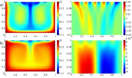
mimicking large cells of warm water and cold water fila-ments observed experimentally in cool skin regime. Steady-state temperature and horizontal velocity fields are shown in figure 11 for Biv = 10 and 2·104. Distances are
nor-malized with respect to tank size. Note that horizontal ve-locity is shown only for the uppermost region up to depth 2 mm in order to reveal the structure of the surface layer. For small values of Biv number the liquid volume is
ef-ficiently cooled with only exception for thermal bound-ary layers at the walls. Marangoni vortices are more in-tense than the Rayleigh vortices. Maximal velocities about 3 cm s−1are observed at water surface. Flow field near the
surface, dominated by Marangoni vortices, consists of pe-riodical currents along the surface with downward sinks at locations of temperature minima. The vertical temperature gradient is decreased by warm water reaching the surface. Generally, this scenario corresponds to experimental ob-servations made in Marangoni convection regime (for pre-heated water or ethanol and other highly volatile liquids). For large Bivmaximal horizontal velocity at the surface
de-creases down to 0.1 mm s−1. Marangoni vortices are weak
tops of two Rayleigh vortices. The cooled layer is much more thin, except for the central sink of cold water pro-vided by Rayleigh convection. Water at the surface is prac-tically motionless, which corresponds to cool skin regime.
Fig. 11. Temperature in entire domain (left column,◦C) and hor-izontal velocity in surface layer (right column, m s−1) for Bi
v =
a) 10, b) 2·104.
No-slip condition and Eq. (5) present extreme cases of boundary condition Eq. (6) for large and small values of Biv, respectively. No-slip condition does not account for Marangoni vortices, whereas Eq. (5) leads to surface liquid velocities of several cm s−1, which is incompatible with regime of motionless cool skin. Boundary condition of third kind Eq. (6) yields temperature and velocity fields similar to those observed in experiments, though the value of Biv number remains an adjustable parameter, which is not derived from properties of liquid and initial (or ambi-ent) conditions. Boundary condition with surface viscosity Eq. (7) is more relevant from physical point of view. Due to presence of velocity second derivative along the surface, it is numerically unstable, which can be fixed by choosing appropriate discretization for this term and performing sev-eral iterations to preserve accuracy. The results, similar to shown in figure 11, are obtained forηsur f ≥2·10−4kg s−1. Note that this value is considerably higher than typically measured in liquid films (10−5−10−7kg s−1[28]). The rea-son of such discrepancy is unclear.
6 Conclusions
Temperature fields under the surface of evaporating liquids were studied by two independent experimental techniques and also by means of numerical simulations. It was shown that, depending on the liquid surface tension and volatility as well as on initial vertical temperature gradient, two dif-ferent structures of surface layer can be obtained: motion-less cool skin and Marangoni convection. The former is characterized by large cells of warm liquid surrounded by filaments of cold liquid and by surface velocity practically equal to zero. The latter implies small cells and moving liquid surface. Cool skin is typical for liquids with large surface tension and/or small volatility, whereas Marangoni convection usually takes place if surface tension is small or
evaporation is intense. Nevertheless, liquids, which typi-cally exhibit cool skin behavior, can be moved into Maran-goni mode by simple preheating, providing large vertical temperature gradient and intense evaporation. On the con-trary, liquids, which usually form Marangoni small-scale cellular structure, can be cooled down to exhibit cool skin. In particular, water, which, as had been reported, does not exhibit Marangoni convection, can be made to do so. Com-parison of the results obtained by BOS and IRTI revealed the lack of spatial resolution of BOS results near the liquid surface. Nevertheless, this technique can be successfully applied to liquid temperature measurements in evaporation problems since the results accuracy is better than 0.1 K. In fact, it is limited by the accuracy of thermocouple, measur-ing the reference temperature, rather than BOS accuracy. Also, this technique is extremely simple and cheap in re-alization and, along with IRTI, can be recommended for outdoor measurements.
The performed numerical simulations demonstrate that air- and water-side problems can be separated with help of IRTI surface temperature data. It is shown that evap-oration rate can be calculated numerically without making use of empirical calculations. This requires solving air-side problem with appropriate boundary conditions at water– air interface: water vapor saturation and fixed water tem-perature or water temtem-perature evolution according to local heat balance equation. Evaporation regime is determined by the value of total Rayleigh number, taking into account both the effects of thermal and concentration-induced con-vection. At high Rayleigh numbers evaporation proceeds chaotically, with plumes of cold humid air formed sporadi-cally at different locations. Universal curves were obtained for Sherwood-Rayleigh relationship in both cases of cold and hot water and compared to known empirical corre-lations. Simulations of water-side problem and compari-son with experimental data revealed the issue of boundary condition for velocity at the surface of evaporating liquid. Boundary condition of third kind was proposed, which en-ables one to model both variants of the surface layer struc-ture. However, it contains one adjustable parameter, which is not derived from liquid properties and/or initial condi-tions. Similar situation is observed for boundary condition involving surface viscosity coefficient: simulation provides results being in agreement with experiment only for sur-face viscosity values considerably higher than found in lit-erature. Future investigations are to solve this problem and to provide physical reasoning for these (or similar) bound-ary conditions. This might require comprehensive study of near-surface rheology since the surface layer is often ob-served to exhibit much more viscous behavior than the bulk liquid.
References
1. K.B. Katsaros, W.T. Liu, J.A. Businger, and J.E. Till-man, J. Fluid Mech., 83, (1977) 311–335
2. P.J. Minnett, M. Smith, and B. Ward, Deep-Sea Re-search Part II: Topical Studies in Oceanography, 58, (2011) 861–868
3. M.M. Shah, Energy and Buildings, 35, (2003) 707– 713
4. W.T. Liu, K.B. Katsaros, and J.A. Businger, J. Atmos. Sci., 36, (1979) 1722–1735
5. W.G. Spangenberg, W.R. Rowland, Phys. Fluids, 4, (1961) 743–750
6. R.J. Volino, G.B. Smith, Exp. Fluids, 27, (1999) 70–78 7. S.J.K. Bukhari, M.H.K. Siddiqui, Phys. Fluids, 18,
(2006) 035106
8. S.J.K. Bukhari, M.H.K. Siddiqui, Phys. Fluids, 20, (2008) 122103
9. S.J.K. Bukhari, M.H.K. Siddiqui, Int. J. Therm. Sci.,
50, (2011) 930–934
10. E.D. McAlister, W. McLeish, Appl. Opt., 9, (1970) 2697–2705
11. G. Meier, Exp. Fluids, 33, (2002) 181–187
12. K. Sefiane, C.A. Ward, Adv. Colloid Interface Sci.,
134-135, (2007) 201–223
13. Yu.Yu. Plaksina, A.V. Uvarov, N.A. Vinnichenko, and V.B. Lapshin, Russ. J. Earth Sci., 12, (2012) ES4002, http://elpub.wdcb.ru/journals/rjes/v12/2012ES000517/ 2012ES000517.html.
14. B. Atcheson, W. Heidrich, and I. Ihrke Exp. Fluids, 46, (2009) 467–476
15. F. Scarano, M.L. Riethmuller, Exp. Fluids, 26, (1999) 513–523
16. W. Wagner, A. Pruss, J. Phys. Chem. Ref. Data, 31, (2002) 387–536
17. P. Schiebener, J. Straub, J.M.H. Levelt Sengers, and J.S. Gallagher, J. Phys. Chem. Ref. Data, 19, (1990) 677–718
18. H.E. Dillon, S.G. Penoncello, Int. J. Thermophys., 25, (2004) 321–335
19. N.A. Vinnichenko, A.V. Uvarov, and Yu.Yu. Plaksina, Proc. of the 15th Int. Symp. Flow Visualization (Minsk, Belarus), (2009) 81
20. K.A. Flack, J.R. Saylor, and G.B. Smith, Phys. Fluids,
13, (2001) 3338–3345
21. M. Al-Shammiri, Desalination, 150, (2002) 189–203 22. S.M. Bower, J.R. Saylor, Int. J. Heat Mass Transfer,
52, (2009) 3055–3063
23. S.J.K Bukhari, M.H.K. Siddiqui, Heat Mass Transfer,
43, (2007) 415–425
24. Z. Li, P. Heiselberg, Aalborg University, Denmark, Report for the project ”Optimization of ventilation system in swimming bath”, (2005)
25. G.A. Nunez, E.M. Sparrow, Int. J. Heat Mass Transfer,
31, (1988) 461–477
26. H.Y. Wong, Author, Handbook of essential formulae and data on heat transfer for engineers (Longman, London, New York 1977)
27. E.M. Sparrow, G.K. Kratz, and M.J. Schuerger, J. Heat Transfer, 105, (1983) 469–475