www.nat-hazards-earth-syst-sci.net/15/1933/2015/ doi:10.5194/nhess-15-1933-2015
© Author(s) 2015. CC Attribution 3.0 License.
Developing system robustness analysis for drought risk
management: an application on a water supply reservoir
M. J. P. Mens1,2, K. Gilroy3, and D. Williams4
1Department of Flood and Drought Risk Analysis, Deltares, P.O. Box 17, 2600 MH, Delft, the Netherlands 2Twente Water Centre, Twente University, P.O. Box 217, 7500 AE, Enschede, the Netherlands
3Institute for Water Resources, US Army Corps of Engineers, 7701 Telegraph Road, Casey Building, Alexandria, VA 22315, USA
4Tulsa District Office, US Army Corps of Engineers, 1645 S. 101st E. Ave., Tulsa, OK 74128, USA
Correspondence to: M. J. P. Mens ([email protected])
Received: 21 October 2014 – Published in Nat. Hazards Earth Syst. Sci. Discuss.: 7 January 2015 Accepted: 12 August 2015 – Published: 26 August 2015
Abstract. Droughts will likely become more frequent, greater in magnitude and longer in duration in the future due to climate change. Already in the present climate, a vari-ety of drought events may occur with different exceedance frequencies. These frequencies are becoming more uncertain due to climate change. Many methods in support of drought risk management focus on providing insight into changing drought frequencies, and use water supply reliability as a key decision criterion. In contrast, robustness analysis focuses on providing insight into the full range of drought events and their impact on a system’s functionality. This method has been developed for flood risk systems, but applications on drought risk systems are lacking. This paper aims to de-velop robustness analysis for drought risk systems, and il-lustrates the approach through a case study with a water supply reservoir and its users. We explore drought charac-terization and the assessment of a system’s ability to deal with drought events, by quantifying the severity and socio-economic impact of a variety of drought events, both fre-quent and rare ones. Furthermore, we show the effect of three common drought management strategies (increasing supply, reducing demand and implementing hedging rules) on the robustness of the coupled water supply and socio-economic system. The case is inspired by Oologah Lake, a multipur-pose reservoir in Oklahoma, United States. Results demon-strate that although demand reduction and supply increase may have a comparable effect on the supply reliability, de-mand reduction may be preferred from a robustness perspec-tive. To prepare drought management plans for dealing with
current and future droughts, it is thus recommended to test how alternative drought strategies contribute to a system’s robustness rather than relying solely on water reliability as the decision criterion.
1 Introduction
1.1 Drought management under uncertainty
Droughts affect more people than any other kind of natu-ral disaster owing to their large-scale and long-lasting na-ture (WMO, 2013). In 2012, losses due to drought in the US were estimated at USD 30 billion (NOAA, 2013), making it the most extensive drought year since 1930. There is a pos-sibility that droughts will intensify in the 21st century due to reduced precipitation and/or increased evapotranspiration (IPCC, 2012). This means that droughts may become more frequent, greater in magnitude and/or longer in duration. Fu-ture uncertainty, combined with natural climate variability, is a challenge for long-term decision making on drought man-agement.
historic droughts (e.g., Watts et al., 2012; Steinschneider and Brown, 2013). However, decision making criteria are lacking to compare and rank various drought management measures. Decision making on drought management often relies on a measure of water supply reliability (Iglesias et al., 2009; Rossi and Cancelliere, 2012): the probability of meeting the water demand. Reliability can be increased by either re-ducing the demand (e.g., by water conservation, reuse of wastewater and reduction of distribution losses) or increas-ing the supply (e.g., by buildincreas-ing new reservoirs, expandincreas-ing existing reservoirs, constructing desalination plants). How-ever, this reliability metric is based on estimates of long-term demand and supply patterns, and does not give insight into the (socio-economic) impact of water shortage once it oc-curs. Besides managing towards an acceptable balance be-tween demand and supply, it is important to understand the impact of temporary situations of water shortage and the ef-fect of short-term measures that aim to reduce these impacts, such as delivery restrictions and/or rationing, temporary ad-ditional sources of supply, and prioritization among users. In addition to long-term supply reliability, decision making criteria are thus needed to provide insight into the effect of drought management measures during droughts. This paper proposes new criteria to support decision-making on drought risk management.
1.2 Analysing system robustness
A method to obtain insight into the impact of a range of hydro-meteorological events on a system’s functioning has been proposed in Mens et al. (2011): system robust-ness analysis. The concept of robustrobust-ness originates from the engineering literature, where it is defined as the abil-ity of systems to maintain desired system characteristics when subjected to disturbances (Carlson and Doyle, 2002). A similar concept, resilience, originates from the socio-ecological resilience community and is defined as the abil-ity of ecosystems or socio-ecological systems to absorb dis-turbances without shifting into a different regime (Holling, 1973; Walker and Salt, 2006; Folke, 2006; Scheffer et al., 2001). Robustness and socio-ecological resilience are com-parable concepts (Anderies et al., 2004), but robustness is considered more suitable for systems in which some compo-nents are designed (Carpenter et al., 2001). Since we focus on water management systems (including drought risk sys-tems), which usually contain many engineering components, we prefer the term robustness. Furthermore, resilience in wa-ter management has been defined as the ability to recover from the impact of flood events (De Bruijn, 2004), which stays closest to its original (latin) meaning: “to jump back”.
In a flood-risk context, systems are disturbed by river flood waves, and they may shift into a different regime when the impact from flooding is too large to recover from (Mens et al., 2011). Resilience, in the narrow definition, can be consid-ered one of the system characteristics that add to a system’s
robustness; the ability of a system to remain functioning de-pends on its ability to recover from the response to a distur-bance. Another characteristic that adds to system robustness is resistance, the ability to withstand disturbances without re-sponding at all (zero impact) (see De Bruijn, 2005).
The robustness analysis method aims to provide insight into the sensitivity of a system to extreme events that result from climate variability, for example floods and droughts. Because climate change may affect the frequency of these events, robustness analysis focuses on a range of events that are plausible both now and in the future. Understanding the relationship between extreme events and their impact on the system is believed to aid in drafting robust strategies that in-crease the system’s ability to deal with both frequent and rare events, now as well as in the future.
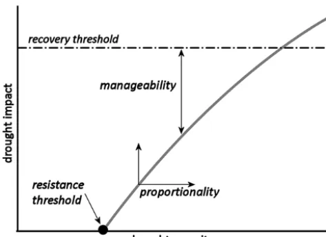
The first step in a robustness analysis is to draw a rela-tionship between drought severity and corresponding impact: the response curve (Fig. 1). This curve visualizes the impacts that can be expected under a range of drought events. Next, the curve is described by the following robustness criteria:
1. Resistance threshold: under which drought conditions will socio-economic impacts first start to occur? In other words: to what extent can the system withstand droughts?
2. Proportionality: how gradual does the impact increase with increasing drought severity?
3. Manageability: under which range of drought condi-tions are impacts still manageable? In other words: when do impacts exceed a societally unacceptable level?
In a flood risk system, the resistance threshold relates to the protection standard. A proportional response curve of a flood risk system implies that sudden impacts are avoided, because a slight change in river discharge does not result in substan-tially different flood impact. Finally, flood impacts are man-ageable when they are below a critical level for a large range of flood magnitudes. The robustness analysis method has been successfully applied on two systems exposed to river flooding, where it was demonstrated that the robustness crite-ria have additional value compared to the more traditional de-cision making criteria based on single-value risk (Mens and Klijn, 2015; Mens et al., 2014).
Figure 1. Example response curve: relationship between drought
severity and drought impact, and robustness criteria
1.3 Application on a drought risk system
To explore the potential of robustness analysis in a drought management context, this paper develops the approach for a system exposed to droughts. The system includes a water supply reservoir and water users. As an illustration of the ap-proach, we apply it on a case inspired by the Oologah reser-voir in Oklahoma, United States. The data available from this reservoir were adapted to be able to show the effect of differ-ent drought managemdiffer-ent strategies (smaller demand, higher capacity, hedging rules) on the robustness.
Oologah Lake is a reservoir northeast of the city of Tulsa, Oklahoma, in the United States. This reservoir was con-structed between 1950 and 1972 as one of many reservoirs aiming at flood control of the Verdigris River. The Verdi-gris River is a tributary of the Arkansas River, which flows into the Mississippi River. Besides flood control, the reser-voir has three other functions: water supply, navigation and recreation. The reservoir is operated such that the water level is low enough to buffer high runoff events (flood control) and high enough to provide a buffer for droughts (water conser-vation). We focus on water supply for municipal use. Ac-cording to historic streamflow measurements, the average an-nual inflow sum is about 2.8×1109m3. The reservoir ca-pacity is about 6.7×10⁸m3. For the purpose of the illustra-tive case, we reduced the reservoir capacity to 5.4×1108m3 (see Sect. 2.2). In this way, a wider range of extreme drought events is available that cause different levels of shortage in water supply.
Drought management strategies lead to new system con-figurations with different characteristics. We consider the fol-lowing strategies:
1. Demand reduction: water demand is reduced on a struc-tural basis, for example by more efficient distributing systems, motivating inhabitants to reduce domestic
wa-ter use, and by rainwawa-ter harvesting (so tap wawa-ter is not used for watering gardens and lawns).
2. Hedging: outflow is temporarily reduced when a criti-cal reservoir level is reached; thereby accepting smaller losses now to avoid major losses later on.
3. Reservoir expansion: the conservation storage is in-creased at the cost of the flood control buffer, making more water available. Demand remains the same as in the reference. No hedging rules apply.
2 Methods and assumptions
2.1 Water balance model and input data
A simple water balance model calculates storage over time as a function of inflow and outflow. The storage is the volume of water in the reservoir that is available for water supply, the inflow is the volume of water per time step flowing into the reservoir, and the outflow is the users’ intake from the reservoir (also a volume of water per time step). In the refer-ence situation no hedging rules are assumed: this means that demand is met until the reservoir is empty. Each simulation assumes a full reservoir at the start. If the conservation stor-age is exceeded, the model releases water accordingly.
Overview of parameters in the reference configuration: – reservoir capacity=5.4×10⁸m3
– required outflow (demand)=17.4 m3s−1.
Parameters for the configurations with alternative drought management strategies:
– S1 Demand reduction from 17.4 to 15 m3s−1
– S2 Hedging: at 25 % storage the outflow is reduced by 60 %
– S3 Reservoir expansion by 20 % (from 5.4×10⁸m3to 6.7×10⁸m3).
Values for S1 and S3 are chosen such that their resulting wa-ter supply reliability (%time outflow > demand) is similar. Implementing hedging rules will reduce the supply reliabil-ity, but will potentially mitigate the severity of impacts over the duration of the event.
the Verdigris catchment. The hydrologic response of Oolo-gah Lake watershed to climate change was analysed by using downscaled climate projections in the variable infiltration ca-pacity (VIC) land surface model. We used the 112 monthly hydrographs from projections of the World Climate Research Program Coupled Model Intercomparison Phase 3 (WCRP-CMIP3), including IPCC’s CO2emission scenarios A1b, A2 and B1. We obtained this set from USBR (2012). The same data set was used by Williams (2013) for his study on the effect of climate change on water availability from Oologah Lake.
This paper does not aim to analyse the effect of climate change on drought and drought impact. Instead, we use the historic and future inflow series to obtain a range of plausible drought events for which the impact can be simulated with the water balance model and the loss functions (described be-low). This will help to obtain insight into how impacts vary with different drought magnitudes, which can be used to con-duct climate risk assessments.
2.2 Characterising and selecting drought events To select drought events from a long time series, differ-ent methods have been developed. Hisdal and Tallaksen (2000) give an overview of the most common methods, for example the threshold level method (TLM) and the se-quent peak algorithm (SPA). The threshold level method as-sumes a user-defined threshold (for example the long-term mean); a drought event occurs when the streamflow is be-low this threshold (Yevjevich, 1967; Dracup et al., 1980). The downside of TLM is that for longer droughts the flow may temporarily exceed the threshold, which divides the longer droughts into smaller mutually dependent droughts (Hisdal and Tallaksen, 2000). To avoid this problem, smaller drought events can be pooled. SPA can be considered a pool-ing method.
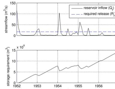
SPA (Loucks and Van Beek, 2005; Vogel and Stedinger, 1987) is an automated equivalent of the Rippl Mass Diagram Approach, one of the first methods to calculate a reservoir’s storage requirement. The design storage of Oologah Lake has been determined with this method as well. We chose this method because it is able to combine consecutive smaller drought events into one large drought event.
With SPA, the required storageKt is calculated over a
pe-riod of record of streamflowQt, given a required releaseRt
(Eq. 1). The design storage equals the maximum value ofKt,
see Fig. 2. Kt=
Rt−Qt+Kt−1 if positive
0 otherwise (1)
The onset (ton)of an event is whereKtbecomes positive, and
the offset (toff)is whereKtreaches its maximum value
(His-dal and Tallaksen, 2000). The event duration is thus defined as:
duration=toff−ton. (2)
Figure 2. Example of sequent peak algorithm: (a) time series of
streamflow (Qt)and required release (Rt), and (b) corresponding storage requirement: the reservoir would be designed based on the maximum value
We can now calculate the drought volume:
volume=
toff X
ton
(Rt−Qt)=Ktoff. (3)
The SPA method was applied on each of the available in-flow time series. For each of the time series, the following steps were taken:
– Selection of periods during whichKt> 0;
– Store start date of each period: the onset of the drought event;
– Find the date whereKt reaches its maximum value: the
offset of the drought event;
– Go back to original streamflow series and select the part from onset to offset; this is the input time series for the water balance model.
Each of the 150-year streamflow time series yielded several drought events with different characteristics (duration and volume).
2.3 Water supply loss function
when there are no shortages), water rate and price elasticity, see Eq. (4) (Dixon et al., 1996).
WTP(Q)=P0(1− 1
η)(Q0−Q)+ P0 2ηQ0
(Q20−Q2), (4) where WTP is willingness-to-pay [USD], P0 is water rate [USD m−3] Q0is baseline water use [m3],Qis water avail-able from reservoir [m3] andηis price elasticity [−].
As suggested by Brozovi´c et al. (2007), we can assume that in case of 100 % water shortage, a government would supply the basic water needs for drinking and sanitation by trucking in water from a different source (e.g., a dif-ferent reservoir). An estimate for trucking cost was taken from the guidebook of the US National Cooperative High-way Research Program in 1995 (NCHRP, 1995). They give an estimate of USD 0.0885 per ton per US mile in the year 1995, including 45 % empty miles. For the year 2013 this equals USD 0.1309 per ton per mile (based on consumer price indices of 152.4 in 1995 and 233.4 in 2013) and USD 0.086 m−3km−1(0.95 m3water weights about 1 ton).
The monthly costs (C) involved with trucking in water are thus:
C(QT)=CT ·x·QT, (5)
where CT is water trucking price [USD m−3km−1], x is
trucking distance [km] andQT is water volume to be trucked
[m3].
The basic water requirement BWR (m3 per month) can be calculated by assuming that 10 % of the baseline munic-ipal water use (Q0) is needed for drinking and sanitation. If the water supplyQfrom the reservoir is less than BWR, we assume that the government will truck in a water vol-ume of (BWR−Q). These are the additional costs on top of WTP(BWR). The total losses associated with water supply deficit (LWS)are calculated by combining Eqs. (5) and (6):
LWS=
WTP(Q)for BWR≤Q < Q0
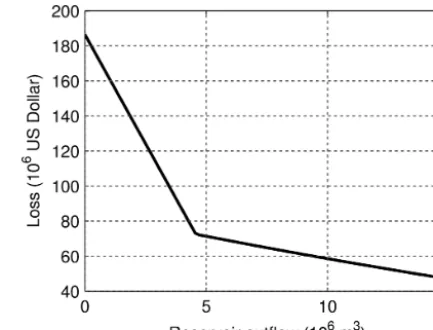
C(BWR−Q) + WTP(BWR) forQ <BWR (6) When reservoir outflowQis smaller than BWR, the govern-ment has a cost of providing enough water to obtain BWR, and individuals have a cost of having less water than their baseline use. In practice, however, it may be technically dif-ficult for a water authority to pump very small amounts of water through their distribution network. The resulting loss function is given in Fig. 3, which shows the loss LWS as a function of reservoir outflowQ.
We used the following values for the case:
– The consumer price for municipal water P0= USD 0.84 m−3(USD 0.00318 per gallon) (Tulsa, 2013); – Average municipal water demand Q0=17.4 m3s−1
(Ref) andQ0=15 m3s−1(S1);
– Price elasticityη= −0.41 (Dalhuisen et al., 2003);
Figure 3. Loss for municipal water users as a function of reservoir
outflow (for 1 month), based on reference water demand
– Trucking distancex=290 km, assuming that water will be trucked in from the Kaw reservoir 145 km (90 miles) away, which is a 290 km roundtrip;
2.4 Scoring the robustness criteria
To draw the response curve of the drought risk system, the disturbance was quantified by the drought volume: the cu-mulative difference between inflow and demand over the du-ration of the drought event. The drought impact (response) was quantified as the total loss in US Dollar as a result of this drought event. The response curve was then used to score the robustness criteria.
The resistance threshold was quantified as the largest drought volume that first causes drought impact. When this is divided by the largest drought volume considered, a value between 0 and 1 is obtained.
The proportionality was scored by visually detecting sud-den changes in drought impact with increasing drought vol-ume. Proportionality is scored high when no sudden changes are detected, and low when the impact increases from zero to maximum impact as a result of a small increase in drought volume.
The manageability was scored by looking at the steepness of the curves. If the curve is less steep than the reference, impacts are smaller and larger drought volumes are needed to cause the same level of impact.
3 Results
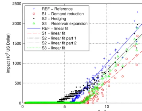
The resistance threshold in the reference is similar to the reservoir capacity. This was to be expected, since the refer-ence assumed no hedging so that drought impacts only oc-cur when the drought volume exceeds the reservoir capacity. This means that the system can withstand drought events un-til a drought volume of 5.4×10⁸m3. The maximum volume of all considered drought events is about 14×108, thus the system can withstand about 40 % of the total drought range considered. The resistance threshold therefore scores 0.4 on a scale of 0 to 1. The water supply reliability of the refer-ence is estimated between 0.96 and 1, depending on the cli-mate change scenario. The supply reliability was calculated for each of the 112 streamflow series (based on projections of future climate). Some of these series did not contain any drought event with a volume exceeding the reservoir capac-ity. This explains the supply reliability of 1. This points to a likely wetter climate according to some of the climate sce-narios, but it does not mean that drought events will never occur in these futures. Because the length of each streamflow series was limited (150 years), it may be a coincidence that extreme drought events with a small occurrence probability did not occur.
The resistance threshold is increased to 0.5 (∼7×10⁸m3), by either reducing demand (S1) or by increasing supply (S3). The supply reliability is increased in both alternatives to 0.98−1. The hedging option (S2) decreases the resistance threshold to 0.35 and the supply reliability to 0.94−1. Because the outflow is temporarily reduced already when there is still water available from the reservoir, impacts start to occur at smaller drought volumes.
The S1 curve is the least steep one of all the curves, point-ing to the fact that a smaller demand (the amount people are used to) also costs less to replace when this amount is lack-ing. Demand reduction thus increases the drought manage-ability, because it takes larger droughts before a societally unacceptable level of drought impact is reached. The S3 curve is as steep as the reference, so manageability is com-parable. However, because of the higher resistance threshold the total impact remains smaller than that of the reference configuration. S3 thus increases the robustness to drought events.
The S2 curve is less steep than the reference curve for small droughts and as steep for more extreme droughts. Thus, the impact is larger than in the reference between about 4 and 7×10⁸m3 drought volume. This is because the out-flow is reduced before the reservoir is empty. At a volume of about 7×10⁸m3the reservoir is empty and impact increases with the same rate as in the reference. However, impacts re-main smaller than in the reference for large drought volumes. Thus, hedging is beneficial in terms of reducing impact due to extreme droughts, but the impact is increased for the more frequent droughts. In sum, the manageability is equal to the reference.
Figure 4. Response curves of the reference configuration (REF) and
of the alternative configurations with implemented strategies (S1, S2 and S3)
4 Discussion, conclusions and recommendations 4.1 Discussion and conclusions
The aim of this paper was to develop system robustness anal-ysis for drought risk management. To that end, the exist-ing framework for robustness analysis, originally developed for floods, was adapted for droughts and illustrated with a drought case. The results showed that different types of mea-sures (demand reduction, supply increase and hedging) score differently on two of the three robustness criteria: resistance threshold and manageability. The third criterion, proportion-ality, did not distinguish between the system configurations. This could however change when different types of measures are considered.
The case clearly showed the different effect of increas-ing water supply and reducincreas-ing water demand. If demand is lower, impacts will start at larger droughts and impacts are lower over the entire range of drought magnitudes. Demand reduction thus scores higher on both resistance threshold and manageability, and is therefore advocated from a robustness perspective. If only the supply reliability (the traditional de-cision criterion) were used, both measures would have been perceived comparable. This means that the decision between these two measures would mainly depend on the cost in-volved (besides side-effects on sustainability criteria such as environmental impact). The robustness criteria show the ad-ditional benefit of demand reduction which may be worth the investment.
thus scores higher on manageability. However, the question is whether the lower score on one robustness criterion out-weighs the higher score on the other robustness criterion. Furthermore, the effect of hedging highly depends on the type of loss function and the demand reduction factor, and could thus be different for other system configurations and other systems.
Although the resistance threshold is scored on a scale be-tween 0 and 1, this does not mean that a score of 1 should be the ultimate goal. The resistance threshold is intended to inform about which range of drought events the system can withstand (zero impact), in this case 40 % of the total range considered. The score is expected to raise awareness about the possibility of larger events (the other 60 % of the total range considered: the “extreme range”) that the system can-not withstand; thus for which impacts are expected. The sec-ond criterion, manageability, then informs about how well the system can cope with the impacts of drought events in the extreme range.
The total range of drought events considered is a subjec-tive choice. In this case it was chosen to select drought events from a long time series of projected streamflow, according to several climate change scenarios. This shows how severe drought events may become, without having to judge about the likelihood of the climate scenarios. How the future will develop is uncertain, but because drought events originate from climate variability (also in the current climate), the pos-sibility of extreme drought events is certain. Thus, it is certain that extreme drought events will occur at some point, but it is uncertain when. Against this background it may be wise to consider a higher level of manageability, since resistance cannot eliminate the certainty of a drought event. Decision makers still have to decide on the range of drought events for which to prepare management plans and the required level of manageability. A system that is robust for the chosen range of events will most likely be robust for even more extreme events as well.
The illustrative case has demonstrated that a robustness analysis provides additional insight into how a system re-sponds to droughts, compared to the traditional decision cri-terion water supply reliability. Because the impact of drought is expressed in economic terms, and a wide range of drought events is considered, the robustness approach fits well with the move towards risk-based drought management. Further-more, the analysis does not depend on assumptions about how the future climate develops; instead it takes into ac-count a wide range of possible drought events resulting from climate variability. We thus consider robustness anal-ysis promising as part of drought risk management under cli-mate change uncertainty.
5 Recommendations
Compared to the applications of the robustness framework on floods (Mens and Klijn, 2015; Mens et al., 2014), the im-pacts in this case were not compared with a recovery thresh-old. Exceeding a recovery threshold means that impacts are unacceptable in the sense that recovery will be very difficult, costly and time-consuming. It is recommended that future drought applications compare the impacts with a recovery threshold.
For future applications it is recommended to take into ac-count the impact on various water users, instead of only mu-nicipal water use. This makes a robustness analysis more interesting, because it allows testing different short-term drought management strategies, for example those that pri-oritize water supply among users during a drought.
Acknowledgements. Thanks are due to the US Army Corps of Engineers (Institute for Water Resources and Tulsa District) for their support in carrying out the research reported in this paper. The work was partially funded by the Netherlands Knowledge for Climate program.
Edited by: M. Parise
References
Anderies, J. M., Janssen, M. A., and Ostrom, E.: A framework to analyze the robustness of social-ecological systems from an in-stitutional perspective, Ecol. Soc., 9, 2004.
Brozovi´c, N., Sunding, D. L., and Zilberman, D.: Estimat-ing business and residential water supply interruption losses from catastrophic events, Water Resour. Res., 43, W08423, doi:10.1029/2005WR004782, 2007.
Carlson, J. M. and Doyle, J.: Complexity and robustness, P. Natl. Acad. Sci. USA, 99, 2538–2545, doi:10.1073/pnas.012582499, 2002.
Carpenter, S., Walker, B., Anderies, J. M., and Abel, N.: From metaphor to measurement: resilience of what to what, Ecosys-tems, 4, 765–781, 2001.
Dalhuisen, J. M., Florax, R. J. G. M., De Groot, H. L. F., and Nijkamp, P.: Price and Income Elasticities of Residential Water Demand: A Meta-Analysis, Land Econ., 79, 292–308, doi:10.2307/3146872, 2003.
De Bruijn, K.: Resilience indicators for flood risk management sys-tems of lowland rivers, International Journal of River Basin Man-agement, 2, 199–210, 2004.
De Bruijn, K. M.: Resilience and flood risk management. A sys-tems approach applied to lowland rivers, PhD, Delft University of Technology, Delft, 2005.
Dixon, L. S., Moore, N. Y., and Pint, E. M.: Drought management policies and economic effects in urban areas of California, 1987– 1992, RAND, Santa Monica, California, USA, 1996.
Folke, C.: Resilience: the emergence of a perspective for social-ecological systems analyses, Global Environmental Change, 16, 253–267, 2006.
Hisdal, H. and Tallaksen, L. M.: Drought event definition, ARIDE Technical Report No. 6, University of Oslo, Oslo, Norway, 2000. Holling, C. S.: Resilience and Stability of Ecolog-ical Systems, Annu. Rev. Ecol. Syst., 4, 1–23, doi:10.1146/annurev.es.04.110173.000245, 1973.
Iglesias, A., Garrote, L., and Martín-Carrasco, F.: Drought risk management in mediterranean river basins, Integrated Environmental Assessment and Management, 5, 11–16, doi:10.1897/IEAM_2008-044.1, 2009.
IPCC: Managing the risk of extreme events and disasters to advance climate change adaptation: A special report of the Intergovern-mental Panel on Climate Change, Cambridge, UK, 2012. Loucks, D. P. and Van Beek, E.: Water resources systems planning
and management: An introduction to methods, models and appli-cations, United Nations Educational, Paris, 2005.
Mens, M. J. P. and Klijn, F.: The added value of system robust-ness analysis for flood risk management illustrated by a case on the IJssel River, Nat. Hazards Earth Syst. Sci., 15, 213–223, doi:10.5194/nhess-15-213-2015, 2015.
Mens, M. J. P., Klijn, F., De Bruijn, K. M., and Van Beek, E.: The meaning of system robustness for flood risk management, Environ. Sci. Policy, 14, 1121–1131, doi:10.1016/j.envsci.2011.08.003, 2011.
Mens, M. J. P., Klijn, F., and Schielen, R. M. J.: Enhancing flood risk system robustness in practice: insights from two river val-leys, International Journal of River Basin Management, 13, 297– 304, doi:10.1080/15715124.2014.936876, 2014.
NCHRP: Characteristics and Changes in Freight Transportation De-mand: A Guidebook for Planners and Policy Analysts, National Cooperative Highway Research Program, Washington DC, 1995. NOAA: Billion-Dollar Weather/Climate Disasters: available at: http://www.ncdc.noaa.gov/billions/events, last access: August 2013.
OECD: Water Security for Better Lives, OECD Publishing, 2013. Qiao, L., Hong, Y., McPherson, R., Shafer, M., Gade, D., Williams,
D., Chen, S., and Lilly, D.: Climate change and hydrological re-sponse in the trans-state Oologah Lake watershed: Evaluating dy-namically downscaled NARCCAP and statistically downscaled CMIP3 simulations with VIC model, Water Resour. Manage., 28, 3291–3305, 2014.
Rossi, G. and Cancelliere, A.: Managing drought risk in water sup-ply systems in Europe: a review, Int. J. Water Resour. D., 29, 272–289, doi:10.1080/07900627.2012.713848, 2012.
Scheffer, M., Carpenter, S., Foley, J. A., Folke, C., and Walker, B.: Catastrophic shifts in ecosystems, Nature, 413, 591–596, 2001. Sivakumar, M. V. K., Stefanski, R., Bazza, M., Zelaya, S.,
Wil-hite, D., and Magalhaes, A. R.: High Level Meeting on National Drought Policy: Summary and Major Outcomes, Weather and Climate Extremes, 3, 126–132, doi:10.1016/j.wace.2014.03.007, 2014.
Steinschneider, S. and Brown, C.: A semiparametric multivariate, multisite weather generator with low-frequency variability for use in climate risk assessments, Water Resour. Res., 49, 7205– 7220, doi:10.1002/wrcr.20528, 2013.
Tulsa water rates: available at: https://www.cityoftulsa.org/ city-services/utilities/rates.aspx, last access: August 2013. USBR: West-Wide Climate Risk Assessments: Projected
Stream-flow, available at: http://www.usbr.gov/WaterSMART/wcra/ flowdata/index.html (last access: August 2013), 2012.
Vogel, R. M. and Stedinger, J. R.: Generalized storage-reliability-yield relationships, J. Hydrol., 89, 303–327, doi:10.1016/0022-1694(87)90184-3, 1987.
Walker, B. and Salt, D.: Resilience Thinking: Sustaining Ecosys-tems and People in a Changing World, Island Press, Washington, 2006.
Watts, G., Christierson, B. V., Hannaford, J., and Lonsdale, K.: Test-ing the resilience of water supply systems to long droughts, J. Hydrol., 414–415, 255–267, doi:10.1016/j.jhydrol.2011.10.038, 2012.
Wilhite, D. A., Sivakumar, M. V. K., and Pulwarty, R.: Man-aging drought risk in a changing climate: The role of na-tional drought policy, Weather and Climate Extremes, 3, 4–13, doi:10.1016/j.wace.2014.01.002, 2014.
Williams, D.: Water Supply Yield Modeling at Oologah Lake (Okla-homa) with Downscaled Climate Projections (draft March 2013), Institute for Water Resources, US Army Corps of Engineers, Tulsa, Oklahoma, USA, 2013.
WMO: The global climate 2001–2010: A decade of climate ex-tremes (summary report), World Meteorological Organization, Geneva, Switzerland, 2013.