Going beyond the flood insurance rate map: insights from flood hazard map co-production

https://doi.org/10.5194/nhess-18-1097-2018 © Author(s) 2018. This work is distributed under the Creative Commons Attribution 4.0 License.

Going beyond the flood insurance rate map:

insights from flood hazard map co-production

Adam Luke1, Brett F. Sanders1,2, Kristen A. Goodrich3, David L. Feldman2, Danielle Boudreau4, Ana Eguiarte4, Kimberly Serrano5, Abigail Reyes5, Jochen E. Schubert1, Amir AghaKouchak1, Victoria Basolo2, and

Richard A. Matthew2

1_{Department of Civil and Environmental Engineering, University of California, Irvine, CA, USA} 2_{Department of Urban Planning and Public Policy, University of California, Irvine, CA, USA} 3_{School of Social Ecology, University of California, Irvine, CA, USA}

4_{Tijuana River National Estuarine Research Reserve, Imperial Beach, CA, USA} 5_{Sustainability Initiative, University of California, Irvine, CA, USA}

Correspondence:Adam Luke (aluke1@uci.edu)

Received: 24 October 2017 – Discussion started: 3 November 2017

Revised: 2 February 2018 – Accepted: 12 February 2018 – Published: 6 April 2018

Abstract.Flood hazard mapping in the United States (US) is deeply tied to the National Flood Insurance Program (NFIP). Consequently, publicly available flood maps provide essen-tial information for insurance purposes, but they do not nec-essarily provide relevant information for non-insurance as-pects of flood risk management (FRM) such as public educa-tion and emergency planning. Recent calls for flood hazard maps that support a wider variety of FRM tasks highlight the need to deepen our understanding about the factors that make flood maps useful and understandable for local end users. In this study, social scientists and engineers explore opportuni-ties for improving the utility and relevance of flood hazard maps through the co-production of maps responsive to end users’ FRM needs. Specifically, two-dimensional flood mod-eling produced a set of baseline hazard maps for stakeholders of the Tijuana River valley, US, and Los Laureles Canyon in Tijuana, Mexico. Focus groups with natural resource man-agers, city planners, emergency manman-agers, academia, non-profit, and community leaders refined the baseline hazard maps by triggering additional modeling scenarios and map revisions. Several important end user preferences emerged, such as (1) legends that frame flood intensity both qualita-tively and quantitaqualita-tively, and (2) flood scenario descriptions that report flood magnitude in terms of rainfall, streamflow, and its relation to an historic event. Regarding desired haz-ard map content, end users’ requests revealed general consis-tency with mapping needs reported in European studies and

guidelines published in Australia. However, requested map content that is not commonly produced included (1) standing water depths following the flood, (2) the erosive potential of flowing water, and (3)pluvialflood hazards, or flooding caused directly by rainfall. We conclude that the relevance and utility of commonly produced flood hazard maps can be most improved by illustrating pluvial flood hazards and by using concrete reference points to describe flooding scenar-ios rather than exceedance probabilities or frequencies.

1 Introduction

actually encouraged risky development in floodplains and coastal zones (Bagstad et al., 2007). Losses from floods and hurricanes in the (US) have tripled over the past 50 years (Gall et al., 2011), and the National Flood Insurance Pro-gram (NFIP) is operating at a deficit of about USD 1 billion annually with a debt of over USD 20 billion owed to the US treasury before considering insured losses from the 2017 hur-ricane season (Pasterick, 1998; Brown, 2016). In fact, prop-erties insured by the NFIP represent the second largest lia-bility of the US federal government after the Social Security program (Gall et al., 2011).

The American Society of Civil Engineers (ASCE) has called for a national strategy to address the escalation of flood losses and threats to public safety, but it reports that the US public and policy makers have been unwilling to take action despite major hurricanes such as Katrina and Sandy (Traver, 2014). The ASCE directive aligns with a global paradigm shift in management philosophy away fromflood controland towardsflood risk management. Flood risk man-agement (FRM) refers to a portfolio of approaches for reduc-ing risk that is not limited to controllreduc-ing flood waters with en-gineered structures but also includes effective land use plan-ning, emergency response, and personal preparedness. Im-portantly, FRM accepts that absolute protection is not possi-ble. Comprehensive FRM reduces the reliance on engineered flood defenses, which is of paramount importance in the US due to the marginal condition of levees and lack of federal resources available for maintenance and necessary upgrades (Traver, 2014). Studies have shown that robust FRM does in-deed lead to significant reductions in fatalities and monetary losses (Kreibich et al., 2017, 2005); however Traver (2014) and Merz et al. (2007) both report that effectively implement-ing FRM relies on stakeholders who understand their expo-sure and also have access to tools that are useful for manag-ing personal, household, and community risks.

Flood hazard maps are the most commonly used tool for flood risk communication and management. In the European Union (EU), member countries are under a mandate to de-velop national flood hazard maps, flood risk maps, and FRM plans based upon the mapped information (Council of Euro-pean Union, 2007). General guidelines for meeting end user needs have been developed based on participatory processes (Meyer et al., 2012; Hagemeier-Klose and Wagner, 2009; Martini and Loat, 2007), which reflect the varying needs of different end users for different types of information, as well as the need for context-sensitive information. For example, Meyer et al. (2012) present distinctions between the mapping needs for strategic planning personnel, emergency manage-ment personnel and the public, and show that geographical factors (e.g., mountains, polders) influence the need for ve-locity data.

In the US, flood mapping is tied to the NFIP and the resulting flood insurance rate maps (FIRMs) delineate the spatial extent of inundation with a 1 and 0.2 % annual ex-ceedance probability (AEP). As a vehicle designed to

ad-minister an insurance program, the FIRM provides essential information for insurance purposes. Properties with feder-ally backed mortgages located within the 1 % AEP flood-plain are required to purchase flood insurance, while the flood elevations associated with the FIRM are used for in-surance underwriting. However, the binary “in or out” flood-plain designation by the FIRMs’thin grey lines have been criticized for presenting flood risk as definitive and therefore discouraging important flood hazard discourse (Soden et al., 2017). Burby (2001) also suggests that the effectiveness of the NFIP is limited because FIRMs lack information neces-sary to integrate flood hazard considerations into local plan-ning. The Federal Emergency Management Agency (FEMA) has recently expanded its mapping efforts through the Risk Mapping Assessment and Planning program (FEMA, 2014), which produces “non-regulatory” flood hazard data such as depth, velocity, and exceedance probability grids in addition to the standard FIRM (FEMA, 2016). However, the avail-ability of non-regulatory flood hazard data is limited, and the system is not configured to align mapping products with context-sensitive needs for decision-making. In fact, there is a need for US-centric studies and guidelines for producing maps that are useful for a variety of FRM tasks, i.e., mak-ing flood hazard data useable for local end users across vast hydrologic and social conditions. Flood mapping technol-ogy has evolved rapidly over the past decade with modern two-dimensional (2-D) hydraulic flood modeling software, computing systems, and increasingly available high-quality data to produce point-wise flood hazard information includ-ing flood depths, velocities, flood forces, and shear stresses (Sanders, 2017). Hence, a key issue is making this advanced and complex modeling output useable in FRM.

recog-United States

Mexico Tijuana, MX

San Diego, CA

Oceanside

Rosarito

(b) Tijuana River watershed

±

High Low Boundary

(a) Tijuana River valley

Tijua_na River _Chan

nel

Pa

cif

ic

Oc

ea

n

U.S. Naval outlying landing field

Imperial Beach

Suncoast Farms Tijuana River

National Estuarine Research Reserve

Tijuana

Playas De Tijuana

San Antonio United States

Mexico

Sm ugg

ler's

Gulch Los

Lau rele_s

Watershed boundaries Smuggler's Gulch

Los Laureles

¦

0 1¼ 2½ 5_km

0 25 50 100_km

(c) Los Laureles

¦

0 ¼ ½_km

M ain

Ch ann_el

±

±

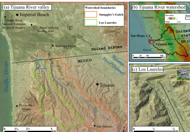
Figure 1. (a)Tijuana River valley and relevant features. The valley is bounded by the city of Imperial Beach to the north, the city of San Diego to the east, and the city of Tijuana to the south.(b)Tijuana River watershed and broader geographical context. Notice the international aspect of the watershed; about one-third of the watershed area is within the US, and the rest is within Mexico.(c)Los Laureles community and Los Laureles main channel. The culvert is also shown, which conveys storm-water discharges from the channelized section of the Los Laureles stream network.

nize the lessons learned from the climate science community by engaging in the co-production of flood hazard maps.

Within the study of engaged scholarship there is a broad spectrum of knowledge “co-production”, depending on the degree of iterativity and duration of scholarly engagement. In this paper, we report a single iteration of a broader co-production effort known as Flood Resilient Infrastructure and Sustainable Environments, which aims to promote resilience to flooding in southern California through continued, mean-ingful efforts of engagement. The goal of the present study is to both deepen understanding about the factors that make flood hazard maps useable at the local scale and to expand the applications of flood hazard mapping via lessons learned from the co-production of flood hazard maps. In order to meet this objective, an interdisciplinary team of engineers and social scientists developed a set of baseline flood haz-ard maps for the stakeholders of the Tijuana River valley in California, US, and Los Laureles in Baja California, Mex-ico (MX). Following baseline hazard mapping by engineers at the two sites, focus groups were held with a diverse group of end users comprised of 52 local professionals and commu-nity members. The focus groups were designed to understand (1) how to improve the clarity and utility of the baseline haz-ard maps and (2) how to re-configure the hydraulic models to produce relevant data and useful maps for the communi-ties. In addition to many map revisions, several original flood hazard maps were produced as a direct result of this iteration of knowledge co-production.

The paper continues with a description of the two study sites involved in the co-production of flood hazard maps (Sect. 2). In Sect. 3, we present the baseline (pre-focus group) flood hazard maps produced for each site. Detailed descrip-tions of the methods used to produce each hazard map are included in the Appendices. Section 4 outlines the implemen-tation and design of our end user focus groups. We present the results of the end user focus groups in Sect. 5.1–5.2, and the new hazard maps that resulted from the focus groups in Sect. 5.3. This paper concludes with a discussion of these sections in the context of previous studies and current flood mapping practice in Europe, Australia, and the US.

2 Study site descriptions

Flood hazard zones

0.2 % annual chance flood hazard 1 % annual chance flood hazard Regulatory floodway

±

(a) FEMA national flood hazard map Tijuana River valley (effective 2012)

Ja_zm ines

±

Los Laureles (effective 2007) Flood hazard zones

Affected zone Flood zone

0 ¼ ½_km

Figure 2. (a)Federal Emergency Management Agency flood insurance rate map for the Tijuana River valley. The orange area represents the flooding extent associated with the 0.2 % annual exceedance probability (AEP) flood, while the blue area represents the flooding extent of the 1 % AEP flood. The red hashed area delineates the regulatory floodway, where development must not increase the designated base flood elevation by more than 0.3 m (1 ft).(b)IMPLAN flood hazard map for the Los Laureles subbasin. The red and blue zones represent inundation extent for different exceedance probability flooding events. However, details regarding mapping methodology and precise hazard zone explanations were not available.

designed to convey spillway discharges from upstream reser-voirs safely through downtown Tijuana. Sediment accumu-lation has reduced the capacity of the Tijuana River channel near the US–MX border and requires dredging to maintain its design conveyance. The TRV has rural housing, an eques-trian (business) presence, and government facilities, but land use in the TRV is primarily preserved for natural habitats or agricultural uses (TRNERR, 2010). Land use in the TRV contrasts the Mexican side of the border, where population density is high due to the presence of coloniasand formal settlements.

LL is a canyon community of Tijuana located south of the US–MX border in the LL catchment (Fig. 1c). The catchment is relatively small compared to the Tijuana River watershed, and flooding is caused by locally intense precipitation. Flows from LL enter the TRV from the south after passing through a small culvert at the watershed outlet. The culvert is fed by a network of concrete lined storm-water channels, which is continually expanding to prevent stream bed erosion and protect adjacent housing developments. The network of con-crete lined channels and expanding urban development has increased the discharges that must be conveyed by the cul-vert. In both study sites, flooding is a known and recurring issue. Engineers from the LL focus groups reported ponding behind the culvert during rainstorms, and a culvert block-age led to severe flooding and subsequent evacuations in LL and southern Imperial Beach. In the TRV, flooding occurs when the upstream reservoirs reach capacity and are forced to open their spillways. Spillway discharges have occurred seven times from 1940 to the present (IBWC, 2006). Indeed, hazard maps which only delineate at risk areas have limited use for locals; stakeholders already know the TRV and LL are

flood-prone. Hazard maps that depict more than the tradi-tional 100-year flood extent are, however, scarce.

3 Baseline flood hazard maps

Baseline flood hazard maps were produced to demonstrate to end users the range of flood hazard data that can be produced with modern methods and to stimulate discussion about haz-ard map improvement and desired content. At this point, it is helpful to define “flood hazard” as the physical and prob-abilistic characteristics of floods. The baseline flood hazard maps therefore depict the intensity of spatially varying prop-erties of floods, such as the depth of flooding for a specified probability. We explicitly define flood hazard to distinguish between maps ofhazardandvulnerability. Merz et al. (2007) define vulnerability as the combination of loss susceptibility and damage potential. Thus, flood vulnerability maps show what could be affected by floods and by how much what is affected could be damaged. We restrict our analysis to flood hazard maps because producing vulnerability maps generally requires data that are unavailable in the absence of extensive surveys. In this study, end users analyzed maps depicting six different flood hazards: depth, force, exceedance probabili-ties, dominant causes, durations, and extents. The proceed-ing section presents the hazard maps analyzed by the end users most applicable to other sites – i.e., we do not present all of the baseline hazard maps herein. The hazard maps we produced were analyzed together with the publicly available hazard maps.

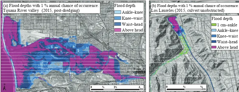
Flood depth Ankle–knee Knee–waist Waist–head Above head (a) Flood depths with 1 % annual chance of occurrence:

Tijuana River valley (2015, post-dredging)

0 ¾ 1½ 3_km

±

Ja_zm ines

±

Los Laureles ( 015, culvert unobstructed)2

Flood depth 1 cm–ankle Ankle–knee Knee–waist Waist–head Above head

0 ¼ ½_km

±

(b) Flood depths with 1 % annual chance of occurrence:

Figure 3. (a)1 % annual exceedance probability (AEP) flood depths in the Tijuana River valley. Mapped flood depths result from either storm tides, canyon flows, or Tijuana River discharges (Appendix A1). The elevation data reflect 2015 topography, after dredging of the Tijuana River channel near the US–MX border.(b)1 % AEP flood depths in Los Laureles. Mapped flood depths are caused by streamflows from local precipitation, assuming that the culvert was unobstructed during the duration of the flood. The depth ranges are 0.11–0.45 m for ankle to knee, 0.45–1.0 m for knee to waist, 1.0–1.69 m for waist to head, and greater than 1.69 m for above head depths.

map for LL is shown in Fig. 2b. Both hazard maps depict the inundation extent associated with different AEPs, while the FEMA FIRM also depicts a regulatory floodway. Develop-ment in the regulatory floodway is prohibited unless the pro-posed structure will not increase the base flood elevation by more than 0.3 m (1 ft). Notice also that the flood hazard is de-scribed by its associated annual probability, which is consis-tent with official FEMA mapping legends and terminology. The IMPLAN Flood Hazard map is similar; areas at risk of flooding are shown, but flooding extent is the only charac-teristic depicted. Flooding extent is also the most commonly mapped hazard in Europe, but many European countries also provide maps of flood depth (de Moel et al., 2009; Nones, 2017).

Figure 3a shows the analyzed flooddepthmap for the TRV, while the depth map for Los Laureles is shown in Fig. 3b. Both maps characterize depths using a body scale and depict depths associated with 1 % AEP events. The body scale is based on the average person height reported by Fryar et al. (2012), with the body part thresholds defined using the 7.5-heads rule from the field of artistic anatomy (Richer, 1986). We use a body scale to contour flood depths with the inten-tion of producing flood hazard data that are more relatable to end users. The clear advantage of providing maps depict-ing the depth of flooddepict-ing is that potentially unsafe areas dur-ing extreme events within the floodplain are easily identi-fied. Figure 3 also demonstrates our (pre-focus group) ap-proach for communicating the mapped hazard. Specifically, we elected to describe flood hazards by their annual proba-bilities and contour intensity of the hazard with a qualitative scale. Data shown on the map other than the flood hazard were limited to allow end users to focus requests and re-visions on the hazard data itself. All of the baseline hazard maps were presented and described in a similar manner.

Figure 4 shows the analyzed flood hazard maps which in-corporate flow velocity information, where the flow velocity, v, multiplied by flood depth,h, is contoured using a scale re-flecting the strength or “force” of the flood waters. We usevh as a proxy for the force of the flood waters because thresh-olds for toppling people and moving cars have been reported in terms ofvh, or discharge per unit width (Xia et al., 2014, 2011). Avhcriterion was also found suitable for predicting structural damage to homes (Kreibich et al., 2009; Gallegos et al., 2012), sovhcan be used to describe a range of haz-ardous conditions. Although the “force” map is more pre-cisely described as a flood discharge per unit width map, we use the word force for simpler communication. By relating the intensity ofvh to the vulnerability of people, cars, and homes, the map could be used for strategic land use planning or emergency response. We note that Australian flood studies produce information describing the severity ofvandh, and recommend that hazard zones are defined byvh thresholds (AEMI, 2013).

The baseline hazard maps were associated with the 1 % AEP event for consistency with the usual presentation of flood hazard information, although each hazard map pre-sented thus far could be produced for an event more or less likely than 1 % AEP. Hazard maps can also display multiple AEP events on a single map. This is accomplished by con-touring the AEP of a particular hazard threshold, rather than contouring the intensity of a flood hazard with a specified AEP.

Intensity of flood force Children toppled Adults toppled Cars sliding

Structural home damage

±

(a) Flood force with 1 % annual chance of occurrence: Tijuana River valley (2015, post-dredging)

0 ¾ 1½ 3_km

±

(b) Flood force with 1 % annual chance of occurence: Los Laureles (2015, culvert unobstructed)

Intensity of flood force

Children toppled Adults toppled Cars sliding Structural damage to homes

0 ¼ ½Kilometers

0 ¼ ½_km

±

Figure 4. (a)Flood force with 1 % annual exceedance probability (AEP) in the Tijuana River valley.(b)Flood force with 1 % AEP in Los Laureles. We usevhas aproxyfor the flood force, since contours are specifically different thresholds ofvh: children toppled at 0.4 m2s−1, adults toppled at 0.65 m2s−1(Xia et al., 2014), cars sliding at 0.8 m2s−1(Xia et al., 2011), and structural damage beginning at 1.5 m2s−1 (Kreibich et al., 2009).

Annual probability

1–2 % 2–4 % 4–10 % 10–20 % 20–50 % > 50 % (b) Annual probability of flood forces that can topple children

Los Laureles (2015, culvert unobstructed)

0 ¼ ½_km

±

±

(a) Annual probability of ankle-depth flooding or greater

Tijuana River valley (2015, post-dredging) Annualprobability

1–2 % 2–5 % 5–10 % 10–20 % 20–50 % 50–90 % > 90 %

0 ¾ 1½ 3_km

Figure 5. (a)Annual exceedance probability (AEP) of ankle-depth flooding in the Tijuana River valley. Contours represent the annual probability that either storm tides, canyon flows, or Tijuana River discharges can cause flooding that exceeds ankle depth.(b)AEP of flood forces that can topple children in Los Laureles. Here, contours represent the annual probability that streamflow will be intense enough to topple children. The ankle-depth threshold was defined as 0.11 m, and the children toppled threshold was defined as 0.4 m2s−1.

results on a single map. The maps shown in Fig. 5 can be produced using a wide variety of hazard thresholds not lim-ited to ankle-depth flooding or children toppled. Here, map-ping exceedance probabilities of a specific hazard threshold quantifies and communicates the likelihood of a particularly negative consequence of flooding. However, the AEP map is difficult to produce (Appendix A3) and presents highly tech-nical information. Thus, it may present challenges in com-municating with end users.

The maps presented in Figs. 2–5 can be produced for a wide variety of locations and are not limited to site-specific hydrologic conditions. We do not present the site-specific baseline hazard maps produced for the end users in this pa-per; however, the site-specific hazard maps illustrating domi-nant drivers and duration of inundation can be viewed online following the links in the “Data availability” section. The

4 Stakeholder focus groups

Four focus groups were held at each study site, which were distinguished by job function related to FRM. The TRV fo-cus groups included 22 total participants, with 6 representing public works professionals and city planners, 8 representing emergency managers, 5 representing natural resource man-agers, and 3 categorized as non-governmental organizations or community. The LL focus groups included 33 participants total, with 9 individuals representing an academic affiliation, 6 representing government, 11 representing emergency man-agers, and 7 representing non-governmental organizations or other community members. Participants of each focus group were recruited through personal communication and referral sampling. It was not possible to strengthen reliability of the focus groups by replicating cohorts because a limited num-ber of individuals are involved with FRM at the study sites. Thus, by limiting our focus groups to individuals who play a role in local FRM, we strengthened the study cohort by including the most relevant participants based on job func-tion. Representation was not identical at the two sites be-cause (1) governmental and organizational structures vary between the two countries and (2) participants were chosen based upon their importance to decisions related to FRM in the respective sites.

The TRV and LL focus groups were each 2.5 h in length, during which a facilitator elicited information regarding the focus group’s perception of the baseline flood hazard maps. A large-format hardcopy of each map was distributed to all participants along with a glossary that described baseline map terms. After individually examining the map, the facil-itator would ask the engineer who produced the map to ex-plain the hazard map and establish a common understand-ing. Participants were able to ask the engineer questions, while the facilitator would ask questions to test understand-ing. Data were generated throughout the focus groups by the facilitator adhering to a script with questions specific to each baseline hazard map. For example, the facilitator would ask participants about their opinions of the indicators used in the map legends, the utility of the mapped hazard data, and infor-mation they would like to see depicted but was not included. This process repeated for each of the baseline hazard maps.

Following the presentation and discussion of the baseline hazard maps, survey data were collected. The surveys were designed to elicit information that would be useful for re-configuring the hydraulic models and producing flood hazard data relevant to the focus group participants. Results from the final “exit” survey addressed several important aspects of producing relevant flood hazard data: end user job func-tion, planning time frames of interest, flood return periods of interest, flood drivers of interest, relevant FRM strategies, and environmental conditions of interest. Each question in the survey was followed by a range of options, and the focus group participants were prompted to select a single option in response to each question.

Data were collected throughout the focus groups by recording conversations and reinforced by note-taking. Fur-thermore, transcripts were prepared of all conversations based on audio recordings. Transcripts were translated into English then analyzed using open coding to identify gen-eral themes and concepts followed by axial coding (cate-gorization) and identification of patterns and relationships among the concepts (Saldaña, 2015; Feldman, 1995). Ex-cerpts from the transcripts were categorized independently using codes including “requested map revisions” and “re-quested map scenarios” to identify end-user-expressed (1) requests for improvements to baseline maps and (2) desired flood hazard map content. Requested map revisions included requests and inquiries related to the map legend, units, and contextual information. Information that was useful for re-configuring the hydraulic models (new scenarios) and pro-ducing new hazard maps were categorized as requested map scenarios. Flood mapping scenarios that were specifically mentioned or requested by participants were verified by in-dependent analysis. Data obtained from the exit surveys were also categorized as requested map scenarios.

5 Results

5.1 Requested map revisions

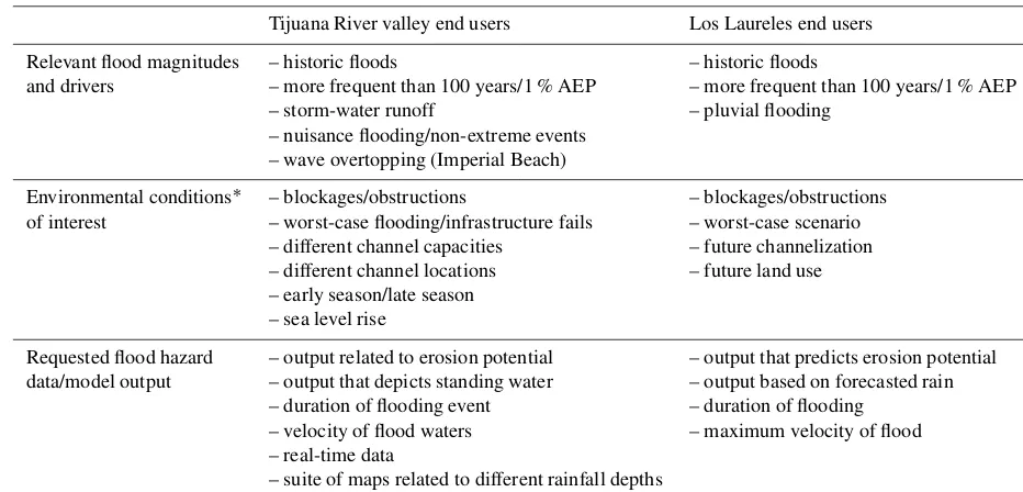
Table 1 summarizes the requested map revisions of the end users from both sites. The requested revisions gen-erally fell into three categories: requests for the hydro-logic/meteorologic conditions of the mapped hazard, further clarification of the map legends, or requests for additional geospatial data to be shown on the map. The requests pre-sented in Table 1 were specifically mentioned by participants and confirmed by discussions recorded in the transcripts.

There were several important requested map revisions that were common to the end users of both sites. First, end users were particularly interested in the amount of rainfall or streamflow that caused the flood hazard on the map. The amount and duration of precipitation leading to the mapped hazard was often requested for both sites, while TRV end users requested the flow rate of the Tijuana River associated with the hazard maps. This illustrates the desire to relate the mapped hazard to information that is available in real time or other publicly available information. LL end users also asked how the mapped scenario related to previous flooding events and noted that the precise frequency of the storm is not nec-essary for many users. Notice that the baseline hazard maps were described by the probability of the mapped hazard only (Figs. 3–5), and not by the conditions leading to the mapped flood hazard such as the amount of rainfall.

Table 1.Summary of the end users’ requested map revisions. These specific requests were identified through transcript content analysis.

Tijuana River valley end users Los Laureles end users

Requested hydrologic/ – amount and duration of precipitation – amount and duration of precipitation meteorologic information – volumetric flow rate – flooding mechanism (cause)

– conditions related to previous flood

Legend requests/ – quantify legend thresholds – quantitative information

comments – scientific units – scientific units

– erosion scale – relate flooding to erosion

– children toppled threshold not appropriate – relate velocity to infrastructure damage – non-technical language

Additional geospatial – access roads – access roads

data requests – river channel – channels

– levees and dikes – population/demographics

– landmarks – sediment basins

– park trails – topography

– sediments and vegetation – aerial photo with year

– locations of dwellings and shelters

basis for the qualitative thresholds. For example, the “chil-dren toppled” hazard criteria (Fig. 4) was received with mixed reactions. Several participants were confused by the distinction between hazardous conditions for children ver-sus adults, which required additional explanation, and others viewed this criterion as alarmist. A participant representing public works professionals said, “I think [children toppled] is an alarming metric. I don’t know if it would be useful for my city work... maybe a different way of identifying inten-sity would be more useful”. Another participant representing natural resource managers noted, “I would be interested in knowing the velocity or what the force impacts are. For what I do, I can’t write in an EIS [environmental impact statement] that a child would be toppled in this area, so that wouldn’t work for me”. End users representing natural resource man-agers were generally more interested in relating the velocity information to the erosive potential of the flowing water, and several participants recommended an erosion scale based on velocity and land cover data. On the other hand, end users representing emergency managers did find the metrics in the force map (Fig. 4) useful.

Emergency managers noted that the flood intensity de-scriptors of the force map would help them decide where to allocate resources during a flood based on the depicted sever-ity, while the “cars sliding” metric would help determine which roads would be inaccessible during an extreme event. Emergency managers also said the force map would help them prepare for hazardous debris flow during a flood: “Let me tell you why this [force map] is really important . . . what I’m really concerned about down in the Valley is . . . anything that’s a hazard in the river that’s actually moving. If I see a barn, and I know that its structural home damage in this area, I’ll be a little more on alert because . . . hey those barns and stuff, they’re gone. And so now I know there’s more things

in the river that not only can create a hazard to me but that can also adjust the flow of the river as well”. Indeed, partici-pating emergency responders were primarily interested in the relative severity of the flood hazard within the floodplain.

Lastly, end users requested a wide variety of additional geospatial data to provide additional context, i.e., infor-mation beyond the illustrated flood hazard. The common geospatial data requests between the two sites included de-pictions of access roads, the river channels, and important flood control infrastructure. Of course, the relevant geospa-tial data will depend on the end user and site-specific charac-teristics, but many end users requested the locations of access roads and river channels.

5.2 Requested map scenarios

Transcripts were examined to extract information that was useful for re-configuring the hydraulic models for new scenarios. This information includes environmental condi-tions of interest, relevant magnitudes and types of flooding events, and requested flood hazard data (model output). Re-configuring and re-running the models involves changes to model inputs such as a topographic data and boundary con-ditions. Table 2 shows the data we collected from the tran-scripts that were relevant for producing the new flood hazard maps.

re-Table 2.Summary of information used to re-run the hydraulic models and produce new hazard maps (requested map scenarios). These specific requests were identified through transcript content analysis.

Tijuana River valley end users Los Laureles end users

Relevant flood magnitudes – historic floods – historic floods

and drivers – more frequent than 100 years/1 % AEP – more frequent than 100 years/1 % AEP

– storm-water runoff – pluvial flooding

– nuisance flooding/non-extreme events – wave overtopping (Imperial Beach)

Environmental conditions∗ – blockages/obstructions – blockages/obstructions of interest – worst-case flooding/infrastructure fails – worst-case scenario

– different channel capacities – future channelization – different channel locations – future land use – early season/late season

– sea level rise

Requested flood hazard – output related to erosion potential – output that predicts erosion potential data/model output – output that depicts standing water – output based on forecasted rain

– duration of flooding event – duration of flooding – velocity of flood waters – maximum velocity of flood – real-time data

– suite of maps related to different rainfall depths

∗_{“Environmental conditions” are defined as the physical conditions of study area or the state of climate related variables during the simulated flood.}

sults (Fig. 6) and the modeling requests documented in the transcripts (Table 2) reveal several important end user prefer-ences and are considered highly relevant to the specific end users in this study.

Regarding the magnitude of the mapped flooding event, end users were interested in events more frequent, or smaller in magnitude, than the 100-year (or 1 % AEP) flood. TRV and LL end users specifically asked to see hazards associated with more frequent events (Table 2), and when asked “What return period is most useful to be mapped?”, more than half of end users from both the TRV and LL focus groups selected return periods of 20 years or less. The 100-year flood was still considered relevant; however end users generally con-sidered the hazards of frequent floods more useful for day-to-day decision making. One participant noted, “We often focus a lot on the 1 % [flood] because of FEMA and things like that, but in terms of what people are experiencing right now, they’re noodling around with like 5- or 10-year events which is what’s causing them problems . . . hitting those frequencies that people are more likely to see, that would be a valuable communication tool”.

Another important finding that was particularly evident from the LL focus groups was interest in the hazards of pluvial flooding, or flooding caused by storm-water runoff. Indeed, twice as many LL end users selected “pooled rain-fall” compared to “excessive streamflow” as the most useful flood driver to be mapped. This interest was documented in the transcripts for both sites, i.e., TRV end users noted that storm-water runoff can cause flooding in neighborhoods just north of the Tijuana River valley. One of the TRV end users

described how nuisance flooding associated with storm wa-ter is noticeably absent from publicly available maps: “We have areas in the city that experience nuisance flooding, and even though it doesn’t show up on the FIRM maps as an area of special flood hazard, . . . you almost have to find out from property owners in there, knock on their doors, [and ask] do you ever get floods here? [owners respond] ‘Oh yeah all the time”’. LL end users were also concerned with flooding caused by storm-water runoff, but they were more interested in flood hazards caused by extreme rainfall events along steep, canyon terraces that are not adjacent to the storm-water channels. Mapping the hazards associated with direct rainfall is considerably different from traditional floodplain mapping, whereby the floodplain is delineated by routing discharges that exceed channel capacities and spread across the floodplain (e.g., Appendix A2–A2.4). Hence, it ap-pears that participating end users astutely discerned a limita-tion of this tradilimita-tional flood modeling approach.

1 year

5 years

10 years

20 years 30 years

50 years 100 years Other (5.3 %)

What return period is most useful to be mapped?

Tijuana River

Smuggler’s Gulch Tide + storm surge Wave driven (5.6%)

What flood driver is most useful to be mapped?

Current conditions

Sedimented channels

Sea level rise

Tijuana urbanization

Los Laureles channelization (5.3 %) Other

What conditions do you most want to see?

15.8 %

15.8 % 15.8 %

1 year

5 years

10 years

20 years 30 years (2.8 %) 50 years 100 years N/A (5.6 %)

11.1 %

Excessive streamflow

Pooled rainfall

Current conditions

Sediment basin at capacity

Changes in rainfall patterns

Obstructions in river channels N/A (2.4 %)

15.8%

5.3 % 5.3 %

10.5 % 31.6 %

15.8 % 10.5 %

11.1 % 11.1 % 16.7 %

16.7 % 25 %

(a) Tijuana River valley end users (b) Los Laureles end users

72.2 %

65.6 % 34.4 %

5.6 % 16.7 %

21.1 %

26.3 % 28.6 % _{31 %}

14.3 % 23.8 %

Figure 6.Results of the exit survey designed to provide insight on relevant flood frequencies, drivers, and environmental conditions. Column (a)includes TRV responses (22 participants), and column(b)includes LL responses (33 participants). The most distinct responses include the reported utility of maps illustrating more frequent events (TRV) and pooled rainfall (LL). The lack of a clear preference for relevant environmental conditions is worth noting. Here, “environmental conditions” are defined as the physical conditions of study area or the state of climate related variables during the simulated flood. Maps depicting possible impacts of climate change (e.g., sea level rise and changes in rainfall patterns) were not the most desired conditions for end users of either site.

change on flood characteristics were not especially relevant to the participating end users. Indeed, LL participants se-lected “changes in rainfall patterns” least frequently when asked “What conditions do you most want to see?”, while sea level rise scenarios were slightly less preferred relative to current conditions in the TRV. Again, these results should not be viewed as representative of all end users of flood hazard data, but it is important to note that these end users did not view climate change impacts on flood hazards as more

rele-vant than scenarios involving infrastructure failures or chan-nel blockages.

Flood depth

1 cm–ankle 0.01–0.11 m Ankle–knee 0.11–0.45 m Knee–waist 0.45–1.0 m Waist–head 1.0–1.7 m Above head > 1.7 m (b) 100 mm of rain in 24 h

(twice the largest observed or 1 % AEP)

Important features Main channel Watershed boundary

±

0 ¼ ½ km

Flood depth 1 cm–ankle Ankle–knee Knee–waist Waist–head Above head (a) Flood depths with 1 % annual chance of occurrence

0 ¼ ½ km

±

Figure 7. (a)Pre-focus group Los Laureles flood depth map based on traditional coupling of hydrologic and hydraulic models.(b) Post-focus group Los Laureles flood depth map based on routing storm-water runoff using the hydraulic model grid. Comparison between(a)and (b)shows that traditional hydrologic–hydraulic model coupling can misrepresent flood hazards in catchments where storm-water runoff is severe. We also present(b)following the stakeholder requests. Notice that(a)is described by the AEP of the flood depths, whereas(b)is described by the amount of rainfall that caused the mapped hazard. The post-focus group map also includes a qualitative/quantitative legend, the location of the main channel, and the watershed boundary.

the flood force map, end users at both sites requested infor-mation describing the velocity of the floodwaters. Aside from maps depicting velocities or erosion potential, end users also requested inundation maps based on real-time information or rain forecasts. One of the participants suggested a collection of maps related to different rainfall depths as a substitute for real-time mapping. Lastly, community members of the TRV requested hazard maps depicting areas susceptible to stand-ing water. Areas susceptible to standstand-ing water are a concern among community members due to increased likelihood of mosquito activity and pollutant exposure. The following sec-tion describes both the new hazard maps and improved pre-sentation of the hazard data that was supported by the end user focus groups.

5.3 Co-produced flood hazard maps

In this section, we present the flood hazard maps that were produced after re-configuring the hydraulic models based on the results of the focus groups. The maps presented herein, Figs. 7–9, do not include all of the maps we produced post-focus group, but rather the hazard maps that both support and expand upon previous studies offering guidance for im-proving flood hazard maps. All hazard maps produced in this study in response to end user feedback can be viewed on-line by following the links in the “Data availability” section. Herein, we also present the mapped hazard data according to the end users’ requested revisions to exemplify effective means of communicating the mapped hazard according to these end users.

First, we focus on end user interest in “pooled rainfall” or storm-water runoff. Figure 7 shows the pre and post-focus group flood depth maps for LL. The pre-focus group flood

depth map (Fig. 7a) was produced by injecting flow hydro-graphs from a hydrologic model into the channel network of the hydraulic model, so the mapped flooded area corre-sponds to so-calledfluvial flooding, or streamflows that ex-ceed the capacity of the channel network (Appendix A2.4). In the post-focus group flood map, on the other hand, runoff (precipitation minus infiltration) was computed for every nu-merical grid of the hydraulic model and routed as overland flow. Hence, the mapped flooded area corresponds to so-called pluvial flooding, or the combined effects of storm-water runoff and excess streamflow. Comparison between Fig. 7a and b reveals that the flood hazard can be significantly underestimated if only fluvial flooding is considered, show-ing the importance of pluvial floodshow-ing (direct storm-water runoff) in this system.

Erodible materials Erosion unlikely < 0.95 N m ² Sandy soils 0.95–3.6 N m ² Fine gravel 3.6–12.4 N m ² Stiff clay 12.4–33.5 N m ² Vegetated surfaces > 33.5 N m ² Erosive potential of 1983 Tijuana River flood (785 m³/s or 5 % AEP)

Important features

Tijuana River crossings Levees and fills

Tijuana River channel (low flow)

0 ¾ 1½ 3

km

±

-Figure 8.Erosion potential map of the 1983 Tijuana River flood produced for the TRV stakeholders. The contoured flood hazard variable is the maximum depth-averaged shear stress predicted by the hydraulic model during the simulated flood event. Legend thresholds were estimated from Fischenich (2001). The map also includes the locations of levees and fills, Tijuana River crossings, and the Tijuana River channel.

a severe rain storm, and from a planning and design perspec-tive, pluvial maps can identify areas in the floodplain with relatively poor drainage.

Notice also that the pluvial hazard map presents the data differently from the baseline map. The pre-focus group map describes the mapped hazard by the exceedance probability of the flood depths, whereas the post-focus group map de-scribes the mapped hazard as the flood depths resulting from the corresponding rainfall depth and duration. In the latter case, the exceedance probability is included but not empha-sized. This may seem like a minor difference, but end users suggested that a description based on rainfall depth is much more useful. Rainfall depths are commonly forecast and re-ported publicly, so the rainfall totals are generally more rele-vant to end users than frequency of occurrence or probability of exceedance. End users’ requests for the amount of rainfall and streamflow associated with the hazard map point to the need to link mapped flooding scenarios to familiar reference points.

Linking flooding scenarios to familiar reference points is difficult, however. Most flooding scenarios are defined by probabilities which are intangible to many end users, while the significance of rainfall totals or volumetric flow rates can be unknown to users not familiar with typical site condi-tions. A reference point requested by end users which has the potential to be accessible to a wide audience was the magnitude of the mapped flooding event relative to historic measurements. Notice that the pluvial flood map (Fig. 7b) also describes the rainfall event as “twice the largest ob-served”, which means the 1 % AEP 24 h rainfall depth is roughly twice the largest recorded at the nearest rainfall gage. Describing the flooding scenario as “twice the largest ob-served” adds important context concerning the magnitude of the mapped event by giving the impression of a rare scenario yet within the realm of physical plausibility.

In addition to the flood hazards caused by storm-water runoff, LL and TRV stakeholders were also concerned about the erosive potential of flowing water (Tables 1 and 2). Ero-sion potential was particularly relevant for the TRV and LL, since highly erosive soils lead to continual dredging of flood control channels and maintenance of engineered sediment basins. Accordingly, we produced maps that illustrate the erosive potential of various floods. Figure 8 shows an ex-ample of an erosion potential map we produced for the TRV stakeholders. The erosion potential map contours the maxi-mum depth-averaged shear stress predicted by the hydraulic model during the course of the simulated flood. We contour shear stress to illustrate erosion potential because shear stress is commonly used to model soil erosion and design stream stabilization or restoration projects (Knapen et al., 2007; Fis-chenich, 2001). The qualitative scale in Fig. 8 that describes materials susceptible to erosion during the simulated flood is based on the permissible shear stresses of different stream restoration materials reported by Fischenich (2001). Notice that the units of the erosion thresholds are also included in the hazard map legend. Although it is unlikely that even tech-nical end users can interpret the magnitude of different shear stress values off hand (i.e., Fig. 8), the units provide the basis for the qualitative scale and improve credibility. The shear stress values by themselves are fairly abstract, so the quan-titative and qualitative scales compliment each other quite nicely.

Water depth Ankle–knee 0.11–0.45 m Knee–waist 0.45–1.0 m Waist–head 1.0–1.7 m Above head > 1.7 m Standing water depth after 2300 m³/s

(triple the 1983 event or 1 % AEP)

Important features

Tijuana River crossings Levees and fills

Tijuana River channel (low flow)

0 ¾ 1½ 3

km

±

Figure 9.Flood hazard map illustrating pooled water that did not freely drain following a peak Tijuana River flow of 2300 m3s−1, which has an estimated 1 % AEP or 100-year frequency. The flood depths shown on the map are the hydraulic model solution after the hydrograph receded to baseflow conditions. The areas that do not freely drain are likely to experience increased mosquito activity and exposure to pollutants following a major flooding event.

(Luke et al., 2015). Maps contouring shear stress and illus-trating erosion potential can be very useful for developing local land use strategies and suppressing erosion. For exam-ple, natural resource managers could restrict sensitive land uses in areas of the floodplain that are likely to experience relatively erosive flows. By overlaying the predicted shear stresses with land use/land cover data, the erosion potential map could also be used to highlight areas in need of armoring or erosion-resistant vegetation.

Notice also that the example erosion potential map dis-plays the shear stresses associated with a hindcast of the 1983 Tijuana River flood, i.e., a historic flood. Stakehold-ers of both sites were interested in hazard maps of historic flooding (Table 2), which we also find particularly valuable due to their relevance to end users and ease of communica-tion. Maps of historic floods are relevant precisely because they actually occurred; the map does not need to communi-cate an abstract exceedance probability or frequency. In the case of historic flood maps, the year of the flood or possibly the name of the storm can be used to describe the flooding scenario. The 1983 Tijuana River flood was associated with a particularly strong El Niño year, which several stakehold-ers recall. The 1983 flood also represents a relatively frequent flood (about 20-year return period) which was deemed use-ful to be shown on a map by end users of both sites (Fig. 6, Table 2).

Lastly, we present one additional flood hazard map pro-duced in response to community members’ concerns about stagnant water in the TRV. Standing water creates breed-ing sites for mosquitos and a correspondbreed-ing proliferation of mosquito-borne diseases such as West Nile virus, so it is an important public health consideration after a major flood (Kouadio et al., 2012). Figure 9 shows the depth of flood wa-ters remaining in the TRV immediately following recession of a flood with a peak flow rate of 2300 m3s−1, assuming no

evaporation or infiltration. Therefore, the map should be in-terpreted as the standing water depth immediately following the flood.

The standing water map is unique relative to other haz-ard maps because it illustrates conditions immediately af-ter rather than during the event and therefore represents a mechanism of supporting ofrecoveryefforts – a key com-ponent of the disaster management cycle (Khan et al., 2008). The standing water map could help authorities with mosquito abatement, deployment of pumps, and strategic positioning of emergency shelters. Additionally, a standing water map can support floodplain planning by enabling enhanced as-sessments of public health risks for proposed floodplain de-velopment projects.

6 Discussion and recommendations

proba-bility. The need for tangible reference points was supported in this study by end users’ requests for the rainfall totals, streamflow, and relative magnitude of the mapped scenario. In flood mapping practice, however, communication of the mapped hazard is still very much tied to probabilities.

The Handbook on Good Practices for Flood Mapping

in Europe (Martini and Loat, 2007) states the title of the map should include the hazard parameter and probability, while the FEMA FIRM describes hazard zones by AEPs only (i.e., Fig. 2). Yet there is increasing evidence that these de-scriptions are ineffective. Relatively little guidance is pro-vided regarding the map legends as well, which is another important aspect of communicating the mapped hazard. Leg-ends are either completely described by numerical values (i.e., depth of flooding in meters or feet) or a qualitative flood severity zone described by terms such as “low” to “severe” (FEMA, 2014). We recommend that future mapping guid-ance documents provide advice for different ways to commu-nicate the mapped hazard scenario and more complete leg-end descriptors. Alternatives supported by this study include (1) providing qualitative and quantitative scales, and (2) de-scribing flooding scenarios by the flood magnitude (in cor-responding scientific units), the magnitude relative to an his-toric event, and finally the probability of the flood. The mag-nitude and probability of the flood provides relevant infor-mation for technical end users, while the magnitude related to an historic event is a tangible reference point for layper-sons. It is our opinion that least emphasis should be given to the probability when describing mapped flooding scenar-ios. Not only are concrete references preferred for describ-ing flood risk (Bell and Tobin, 2007), but flood probabilities and corresponding frequencies are highly uncertain (e.g., Ap-pendix A1.1–A1.3; Di Baldassarre et al., 2010; Kjeldsen et al., 2014; Merwade et al., 2008; Merz and Blöschl, 2008; Stedinger and Griffis, 2008). Indeed, all hazard variables il-lustrated in flood maps are inherently uncertain; however, it is remarkable that perhaps the most uncertain and complex characteristic of floods is also the primary descriptor.

Uncertainties associated with flood mapping products are rarely quantified let alone communicated, and in this study, we did not address the important issue of communicating uncertainty in flood maps to end users. In one of the few studies that has explicitly addressed communicating uncer-tainty in the FEMA FIRMs’ floodplain boundaries, Soden et al. (2017) showed that providing end users with con-trasting information (i.e., the 1 % AEP flood extent versus an observed flooding extent) led to important flood hazard discourse and curiosity regarding flood mapping methodol-ogy. While it may seem counterintuitive to purposefully ex-pose the limitations of floodplain delineation, such innova-tive communication strategies force end users to confront the deterministic standards that our institutions require for reg-ulatory purposes. Explicit confrontation with the limits of science promotes contemplation and is certainly worth

fur-ther investigation in the context of flood hazard mapping and communication.

Regarding desirable content of flood hazard maps, stake-holder preferences from this study also align with previous work. Meyer et al. (2012) concluded that maps presenting flood hazards at different probabilities is required, velocity information should be provided when available, and the loca-tion of flood defenses and access routes should be integrated within the hazard map. All of these recommended contents were requested by the TRV and LL end users. Hagemeier-Klose and Wagner (2009) also noted the importance of map-ping more frequent events than the 1 % AEP flood, which was strongly supported by the results of the survey (Fig. 6). Thus, this study demonstrates consistency between the de-sired map content of end users studied in the US, Mexico, and Europe. Flood mapping guidelines in Europe (Martini and Loat, 2007) and Australia (AEMI, 2013) generally rec-ommend producing this desired content. Guidelines either recommend or require the production of hazard maps associ-ated with different probabilities and even infrastructure fail-ure scenarios. Mapped data include flooding extent, depths, velocities, and the depth–velocity product, while some stud-ies even provide shear stresses (Martini and Loat, 2007). Spe-cific guidance is also provided for producing maps that sup-port the FRM activities of distinct European and Australian end user groups.

Meanwhile, in the US, flood mapping guidelines are fairly extensive and standardized for producing the FEMA FIRM only (FEMA, 2016). There is a lack of guidance and di-rection available for producing flood hazard maps that sup-port non-insurance aspects of FRM, such as those specifi-cally requested by end users in this study. The required “non-regulatory” data products of recent FEMA Risk Mapping As-sessment and Planning studies (FEMA, 2014) have signif-icant potential to support an expanded portfolio of action-able flood hazard maps in the US. For example, the required velocity grids in Risk MAP studies can be post-processed to produce erosion potential maps, while the required “flood severity grid” contains the depth–velocity data necessary for products designed to support emergency response. We rec-ommend that future FEMA guidelines provide specific di-rectives for producing non-regulatory flood hazard maps tai-lored to specific FRM objectives including land-use plan-ning, emergency management, and public awareness. The content of flood hazard maps should also be expanded to in-clude pluvial flood hazards when appropriate.

rela-tively new, guidance documents do not require the produc-tion of maps depicting the pluvial hazard or intense storm-water runoff. Since techniques for estimating pluvial hazards continue to advance, formal guidelines and requirements for mapping the pluvial hazard zone should be developed, espe-cially in the US. As demonstrated by end user requests in this study – and the largely pluvial nature of the flooding disaster caused by Hurricane Harvey in the US – pluvial flooding can dominate in urban areas and needs to be considered in future mapping efforts.

7 Conclusions and future directions

Two-dimensional (2-D) flood hazard models developed for the Tijuana River valley (TRV) and Los Laureles (LL) on both sides of the US–Mexico border supported the co-development of flood hazard maps responsive to end user management needs. Two-dimensional modeling by engineers produced a set of baseline maps that were further refined through end user focus groups that triggered additional mod-eling scenarios and map revisions.

This study revealed general consistency between the map-ping needs of studied end users in the US and Mexico with those reported in European studies and guidelines published in Australia. For example, mapping requests included scenar-ios with different probabilities and even infrastructure fail-ure scenarios, and end users also requested maps of hazard variables beyond traditional flood extent, such as velocities and standing water. This study also revealed several impor-tant flood hazard mapping requests relevant to other sites:

– Flood intensity scales (e.g., depth, force or shear stress) that frame the mapped information both quantitatively and qualitatively. The quantitative scale meets end user needs for a technical reference point, while the quali-tative scale meets end user needs to easily interpret the mapped information.

– Flood scenario descriptions that report both the mag-nitude of the flood in terms of rainfall or streamflow amounts and also the flood magnitude relative to an historic event. Use of concrete scenario descriptions in-creases the utility and relevance of mapped information across different end users of flood hazard maps. – Flood hazard maps that depict the erosion potential of

flood waters. Erosion potential maps support end user needs for managing sediment.

– Flood hazard maps that depict standing water following the flood. Standing water maps support recovery plan-ning and public health concerns.

– Flood hazard maps that depict storm-water runoff or pluvial flood hazards. Baseline flood hazard maps de-pictedfluvialflooding hazards only, and after end user

focus groups revealed a deficiency in usefulness, the need for a pluvial flood hazard modeling approach was recognized and implemented. Characterizing plu-vial flood hazards is extremely important for urbanized sites with poor drainage.

Of course, the stakeholder preferences herein must be viewed cautiously, since focus group participants do not represent all end users of flood hazard data. The primary limitation of this study is the limited number of focus group partici-pants (55 total) and narrow geographic scope. Co-production efforts via focus groups acknowledge that community-level knowledge (and mapping preference) varies from locality to locality, underscoring how flood hazard knowledge should not be a “one-directional” process but an iterative learning approach that breaks down information gaps between ex-perts and lay users in specific places – thus improving risk communication at the local level. They also produce action-able mapping information useful for reducing flood risks (Spiekermann et al., 2015; de Moel et al., 2009). Indeed, restricted sample size and geographic scope is a common caveat of flood communication and mapping preference stud-ies (e.g., Hagemeier-Klose and Wagner, 2009; Meyer et al., 2012).

In future studies, sample size limitations may be overcome by taking advantage of online information systems to present flood hazard data, such as those demonstrated in the “Data availability” section of this paper. Online formats offer the opportunity for causal experiments – do different hazard vari-ables make a user more (or less) likely to seek vulnerability reduction measures? How do different presentations of un-certainty in mapped data influence end users’ desire to seek further information? These questions could be answered with so-called “A/B” testing, where subjects are presented dif-ferent web pages and their interactions on the web site are recorded. Our current knowledge of flood mapping prefer-ences and hazard perceptions is based upon empirical stud-ies with relatively small samples (Kellens et al., 2013). What can “big data” tell us about how end users respond to, and interact with, flood hazard data?

with actionable information. To be actionable, map informa-tion must help decision-makers (1) understand vulnerability of properties from flooding and (2) select actions that miti-gate or reduce this vulnerability (Demeritt and Nobert, 2014; McNutt, 2016; Feldman et al., 2008). By fully utilizing flood modeling technologies and developing innovative commu-nication strategies, flood hazard maps can more effectively support first responders, natural resource managers, and lo-cal residents with the information necessary to manage and respond to flood hazards.

Appendix A: Flood hazard mapping methodology The flood hazard maps presented in this study resulted from three distinct tasks: flood frequency analysis (FFA), hydro-logic and hydraulic modeling, and post-processing of model output. Generally speaking, FFA estimates the recurrence in-terval of rare flooding events, while hydrologic and hydraulic modeling predicts the hazards associated with simulated floods (depths, velocities, extents, etc.). In this study, post-processing methods are used to combine the results of multi-ple simulations onto a single map. The following sections outline our FFA, hydraulic modeling, and post-processing methods so that the interested modeler can produce the haz-ard maps presented herein.

A1 Flood frequency analysis

FFA is complicated in the coastal zone due to the multiple causes or “drivers” of flooding. In this study, we mapped flooding caused by extreme ocean levels, streamflow from the Tijuana (TJ) River, and precipitation over Los Laureles and Smuggler’s Gulch watersheds (Fig. 1). The presence of multiple flood drivers often warrants a multivariate approach for FFA (Salvadori and De Michele, 2013). Under this ap-proach, multivariate extreme value analysis (EVA) is used to estimate the probability of scenarios where multiple ex-tremes occur simultaneously. However, we did not conduct multivariate EVA in this study because of the low correlation between flood drivers and the lack of emergent flood hazards caused by the joint occurrence of extremes.

Table A1 presents the Pearson’s correlation coefficient ma-trix between the flood drivers considered herein. The rela-tively low correlation is somewhat surprising but understand-able. Extended periods of above average rainfall in the upper TJ River watershed cause large streamflow events, whereas relatively short-lived coastal storm systems can elevate ocean water levels and lead to intense precipitation. The low corre-lation between flood drivers demonstrates that the simultane-ous occurrence of extreme events would be especially rare. Perhaps more importantly, hydraulic model sensitivity anal-ysis revealed that predicted flood depths, extents, and veloci-ties are insensitive to the joint occurrence of extremes in this system. For example, flood depths predicted by the hydraulic model are not sensitive to the downstream ocean level during large TJ River floods. The lack of “sufficient” correlation be-tween drivers and the hydraulic model’s insensitivity to the joint occurrence of extremes allows us to consider the flood drivers independently and use univariate EVA for frequency analysis.

A1.1 Tijuana River flood frequency analysis

FFA of TJ River flows was based on a Pearson type III (PIII) distribution fitted to the historic record of log-transformed annual maximum discharges. This approach is consistent

Table A1.Pearson’s correlation coefficient matrix between the three drivers of flooding considered in this study. The numeric values in the table describe the correlation between the variables in the row and column headings. Correlation coefficients were determined us-ing de-trended tide gage data at La Jolla (NOAA station 9410230), precipitation measurements from the San Diego International Air-port (NOAA network ID GHCND:USW00023188), and TJ River streamflow measurements at the US–MX border recorded by the International Boundary and Water Commission.

Ocean TJ stream Precipitation level flow (24 h sum) (daily (daily

mean) mean)

Ocean level (daily mean) 1 0.12 0.21 TJ Streamflow (daily mean) 0.12 1 0.17 Precipitation (24 h sum) 0.21 0.17 1

with the recommended FFA methodology in the US (Hydrol-ogy Subcommittee, 1982). The data record originated from TJ River flow measurements at the US–MX border reported by the International Boundary and Water Commission. To infer the parameters of the PIII distribution, we used the Bayesian parameter estimation technique described by Luke et al. (2017), where an informative prior was used to incor-porate regional information about the skewness of the PIII distribution. For the TJ River, parameter estimation was com-plicated by signs of nonstationarity in the historic record, or time variant statistical properties of the annual maximum dis-charge data.

Figure A1a shows the full data record at the US–MX bor-der. At the time of this study, data were not available af-ter 2006. The black line in Fig. A1a denotes the year when the TJ River channelization was completed, which appeared to alter the mean and standard deviation of the flood peaks. Indeed, the pre-channelization distribution is different from the post-channelization distribution at the 0.05 significance level according to the two-sample Kolmogorov–Smirnov test (Massey Jr., 1951). Due to the apparent change in the distri-bution of flood peaks following channelization, we did not use data prior to 1979 for estimation of the PIII parameters. The choice to omit data prior to channelization creates a rel-atively small sample size for parameter estimation and leads to large variance in the estimated return periods (Fig. A1b). Assuming stationarity following the channelization, the re-turn periods in Fig. A1b are simply the inverse of the annual exceedance probabilities associated with the return levels on theyaxis. If the pre-channelization flood peaks are included in the frequency analysis, we risk bias in the parameter esti-mates and resulting return periods.

Year

1960 1970 1980 1990 2000

Discharge (m

s

)

-3

0 200 400 600 800 1000 1200

(a)

Channelization complete Annual max. discharge

Return period (years)

0 20 40 60 80 100

Return level (m

s

)

-3

101 102 103 104 105

(b)

Most likely PIII fit 95 % confidence interval Empirical estimate

-1

-1

Figure A1. (a) Annual maximum discharge record of the TJ River. Only flood peaks post-channelization were used for PIII parameter inference.(b)Flood frequency estimates derived from the PIII distribution fitted to the log-transformed discharge data from 1979 to 2006. Notice the large variance in flood frequency estimates.

from 1979 to 2006 but did not affect the majority of the relatively small, runoff-driven annual maximum events. The various flood generating mechanisms and the change in the shape of the empirical frequency curve both indicate that the distribution of flood peaks is not the same for small and large annual maximum events. This causes a poor fit of the PIII distribution to the data in the modern period of record and creates even more variance in the frequency estimates. It is unlikely that the variance can be significantly reduced with-out expanding the sample size through watershed modeling and simulation of peak flows, which was outside the scope of this study. It is very important to note that exceedance prob-abilities and corresponding frequency estimates based on the historic TJ River discharges alone are unavoidably uncertain. A1.2 Extreme ocean level frequency analysis

Extreme ocean levels near the TRV also showed signs of non-stationarity in the historic data record. Figure A2a shows the annual maximum compared to the annual mean ocean lev-els recorded at the La Jolla tide gage in CA, US. There is a statistically significant trend in both the annual maximum and mean data at the 0.05 significance level, according to the Mann–Kendall trend test for monotonic trends (Mann, 1945; Kendall, 1976). The persistent trend in ocean levels is not surprising; however it does complicate EVA. In this study, we explicitly modeled the change in extreme ocean levels using a nonstationary, generalized extreme value (GEV) dis-tribution:

X∼GEV(µt, σ, ξ ) , (A1)

where the random variableXis the annual maximum ocean level, andσ andξ denote the scale and shape parameter of the GEV distribution, respectively. The time-variant location parameter,µt, is formulated as a function of changes in mean

sea level,

µt=1MSLo+µo, (A2)

where1MSLois the change in annual mean sea level

rela-tive to the mean during the 1983–2001 tidal epoch, andµois

a constant offset between the location of the GEV distribu-tion and mean sea level. This model was proposed by Obey-sekera and Park (2012) to provide a method for synthesizing extreme value statistics with sea level rise scenarios. We es-timated the parameters of the GEV model using Bayesian parameter inference, again with an informative prior on the shape parameter,ξ. The prior onξ was specified as a nor-mal distribution centered at the La Jolla gage estimate ofξ reported by Zervas (2013). Following parameter estimation, exceedance probabilities of extreme ocean levels are esti-mated as a function of change in mean sea level.

Figure A2b shows extreme water levels versus exceedance probabilities obtained from the fitted GEV model in the year 2015. Notice that along thex axis, we no longer use return periods to describe the frequency of extreme ocean levels. The common definition of a return period relies on the assumption that exceedance probabilities are time-invariant, which is very unlikely due to anticipated changes in future mean sea level. For our hazard mapping purposes, we used the nonstationary model to estimate the exceedance proba-bilities of extreme ocean levels associated with present-day mean (2015) sea level. The fitted model could also be used to estimate exceedance probabilities associated with future sea levels by using sea level rise projections to define1MSLo.

A1.3 Precipitation frequency analysis