Abstract— The subject of control system design has evolved considerably over the years. Although several design techniques and strategies have been adopted to realize control systems that meet a predetermined set of performance criteria, the fundamental problem remains that of developing controllers to adjust the performance characteristics of a dynamic system in order to obtain a desired output behavior. The dynamic behavior of a magnetic levitation system (MLS ) of a ferromagnetic ball is compensated in this paper. Consolidating the exposure of undergraduate students to the rudiments of control system design, the paper employs the classical root locus technique to stabilize the system. A combination of analytical and software -based methods is used to design proportional-derivative and phase-lead compensators based on the linearized model of the system. Complete details of the design approach, from modeling and analysis of the plant to computing the values of the controller parameters, are shown. MATLAB scripts for plotting root loci and simulating the system are provided.
Index Term— compensators, magnetic levitation system, MATLAB® scripts, modeling, root-locus method, system stability
I. INT RODUCT ION
THE magnetic levitation system has attracted a great deal of attention both in the industry and academia. In the industry, significant applications, such as passenger train levitation, magnetic bearing, metal sheet levitation, protection of sensitive machinery, etc., have been recorded, while in the academia, authors of books on control systems theory [1], [2] have used similar versions of the system to educate undergraduate students on the subject of control systems, with laboratories having prototypes and experimental models of the system handy for instructional purposes [3], [4]. The magnetic levitation system of a ferromagnetic ball has a complex nonlinear dynamic equation, and its characteristic response inherently unstable [5]. Successful efforts have been made to design nonlinear controllers [6] just as well as linear
A. A. Awelewa is with the Electrical & Information Engineering Department, Covenant University, Canaan Land, Ota, Ogun state, Nigeria (phone: +234-8062361966; e-mail :[email protected],ng.
I. A. Samuel and Abdukareem Ademola are with the Electrical & Information Engineering Department, Covenant University, Canaan Land, Ota, Ogun state, Nigeria (e-mail: [email protected];
S.O. Iyiola is a final year student in the Electrical & Information Engineering Department, Covenant University, Canaan Land, Ota, Ogun state,
Nigeria.
controllers [3], [4], [5] to stabilize the system. This latter type, which is further considered in this paper, is based on the linearized version of the system operating in a small range around an operating point. The aim of the paper is to shed more light on the us e of a classical technique in stabilizing a magnetic levitation system. The rest of the paper is arranged as follows. Section 2.0 considers the complete modeling of a magnetic levitation system, with both nonlinear and linearized models treated in detail. Section 3.0 focuses on the magnetic levitation system design and simulation, and also, shows graphical displays to buttress design results. And finally, Section 4.0 presents the conclusion. All the MATLAB scripts used for the design and simulation are separately given in the appendix.
II. MAGNETICLEVITATIONSYSTEMMODELLING
A. Layout of the System
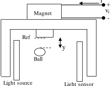
The layout of a typical magnetic levitation system is illustrated in Fig. 1 [6]. This arrangement involves the adjustment of magnetic energy or force in order to balance or counteract the gravitational pull exerted on an object (a small light ferromagnetic ball in this case).
Restricted to the vertical direction only, the motion of the ball is monitored by a properly arranged pair of a light emitter and a light detector so that the instantaneous position of the ball can be fed back for the purpose of control computation. This control effort (generated by an electromagnetic circuit) is to ensure that the ball is brought to, and kept at, a desired position. As the ball‘s position deviates, due to an external disturbance, from the set point, the sensor output changes accordingly so that the right amount of control effort is computed and used to bring the ball back to the set point and keep it there.
Fig. 2 is the repres entation of the electric circuit subsystem of the magnetic levitation system. It is a series combination of a linear resistor, with resistance R, and a non-linear inductor, with inductance L(y).
An Undergraduate Control Tutorial on Root
Locus-Based Magnetic Levitation System
Stabilization
The inductance is non-linear due to the variable reluctance of the magnetic circuit—the reluctance is directly proportional to the distance between the electromagnet and the ball, implying that as this distance decreases (i.e., ball‘s approaching the magnet), the inductance increases, and vice versa.
B. Non-linear Model of the System
To determine the complete model of this system, two important dynamic equations, one representing the variations of the magnetic flux with time (based on Fig. 2) and the other the Newtonian equation of motion of the ball based on forces acting on it as shown in Fig. 3, are required.
From Fig. 2, it can be written that
i
v
)
t
(
Ri
dt
)
y
,
t
(
d
(1)
where Ф(t, y) is the magnetic flux in webers, i(t) is the current in amperes, R is the resistance in ohms, vi is the source voltage
in volts, and t is time in second.
Since the magnetic flux around a coil is directly proportional to the current flow in the coil, with the coil inductance being a factor of proportionality, thus,
)
t
(
i
)
y
(
L
)
y
,
t
(
(2)
Differentiating (2) with respect to time and substituting the result into (1) yield
i
v
Ri(t)
.i(t)
dt
dy
.
dy
dL(y)
dt
di(t)
L(y)
or
i
v
)
t
(
i
dt
dy
dy
)
y
(
dL
R
dt
)
t
(
di
)
y
(
L
(3)
where y(t) is the distance between the electromagnet and the ball, and L(y) is the total inductance of the circuit in henry. Also, from Fig. 3,
F
a+ F
e= F
g(4)
where Fa is the accelerating force due to the mass of the ball,
Fe is the magnetic force, and Fg is the gravitational force.
Since
2
dt
y
2
d
m
a
F
and
mg
g
F
,
therefore, (4) can be rewritten as
e
F
mg
2
dt
y
2
d
m
or
e
F
mg
dt
dv
m
In (5), m is the mass of the ball in kg, v( =
dy
dt
) is thevelocity of the ball in m/s, and g is the acceleration due to gravity in m/s2.
Equations (3) and (5), which constitute the mathematical representation of the system, can be developed further by redefining L(y) and Fe and finding appropriate expressions for
them, respectively, as shown by the following derivations. L(y) represents the sum of two inductances, Lc and Lb, i.e.,
L(y) = L
c+ L
b(6)
Lc, which is fixed, is the inductance due to the electromagnet
coil; Lb is the inductance due to the ball. Because Lb is
inversely proportional to the distance between the electromagnet and the ball, it implies that if Lo is the
inductance that corresponds to a set-point position, yo, then the
inductance, Lb, that corresponds to an instantaneous position,
y, is expressed as
y
o
y
o
L
b
L
(7)
Therefore, putting (7) in (6) gives
y
o
y
o
L
c
L
)
y
(
L
(8)Further, the magnetic force, Fe, is defined as the rate of change
of work done with distance as the ball is moved from one position to the other by the force, and is given as
Fig. 1. Schematic of a magnetic levitation system.
Light sensor Light source
v
i+
-
i
Magnet
y
Ref
Ball
L(y)
-
v
i+
R
i(t)
Fig. 2. Electric circuit subsystem of the maglev system.
Fe
Fa
F
g
dy
dW
e
F
(9)
where, W (the energy stored in the magnetic field) is
2
i
)
y
(
L
2
1
W
Hence, (9) gives
2
y
2
i
o
y
o
L
2
1
e
F
(10)
which, with Lo and yo fixed, can further be reduced to
2
y
2
i
K
e
F
(11)where K (called the magnetic force constant) =
L
o
y
o
2
1
Now, substituting (8) into (3), and (11) into (5), we have
i
v
)
t
(
i
dt
dy
2
y
o
y
o
L
R
dt
)
t
(
di
)
y
(
L
(12)
and
2
y
2
i
K
mg
dt
dv
m
(13)
The final non-linear equations are
i
v
)
y
(
L
1
)
t
(
i
v
2
y
K
2
R
)
y
(
L
1
dt
)
t
(
di
(14)2
y
2
i
m
K
g
dt
dv
(15)Let state variables and the input be defined as:
i
v
u
;
i
3
;
v
dt
dy
2
;
y
1
x
x
x
The equivalent nonlinear state-space dynamic model of the system is:
.
3 22
1
2
)
y
(
L
K
2
)
y
(
L
R
u
)
y
(
L
1
dt
3
d
2
1
3
m
K
g
dt
2
d
dt
1
d
x
x
x
x
x
x
x
x
x
(16)
C. Linearized Model of the System
As can be seen in the model just developed, the maglev system is non-linear. As mentioned earlier, several non-linear controllers have been designed for this system in the literature. But the focus here is on how to improve the system performance for small-range operation. Therefore, the above non-linear model is linearized about a nominal operating point, xo(t), which corresponds to a nominal input, uo, using a
Taylor series [7].
First, the model in (16) is rewritten as
(17)
Then expanding (17) into a Taylor series about xo(t) = [xo1, xo2,
xo3] and ignoring terms of order higher than first result in
)
o
u
u
(
o
u
),
t
(
o
u
)
u
,
3
,
2
1
i
f
)
3
o
3
(
o
u
),
t
(
o
3
)
u
,
3
,
2
1
i
f
)
2
o
2
(
o
u
),
t
(
o
2
)
u
,
3
,
2
1
i
f
)
1
o
1
(
o
u
),
t
(
o
1
)
u
,
3
,
2
1
i
f
o
u
),
t
(
o
)
u
,
3
,
2
1
i
f
dt
i
d
x
x
x
,
(x
x
x
x
x
x
x
,
(x
x
x
x
x
x
x
,
(x
x
x
x
x
x
x
,
(x
x
x
x
,
(x
x
(18) where i = 1, 2, 3.
Hence,
)
o
u
u
(
L
1
)
3
o
3
(
2
1
o
L
2
o
K
2
L
R
)
2
o
2
.(
2
1
o
L
3
o
K
2
)
1
o
1
.(
3
1
o
L
3
o
2
o
K
4
dt
3
o
d
dt
3
d
)
3
o
3
.(
2
1
o
3
o
m
K
2
0
)
1
o
1
.(
3
1
o
2
3
o
m
K
2
dt
2
o
d
dt
2
d
0
0
)
2
o
2
.(
1
0
dt
1
o
d
dt
1
d
x
x
x
x
x
x
x
x
x
x
x
x
x
x
x
x
x
x
x
x
x
x
x
x
x
x
x
x
x
(19) Noting that
),
3
,
2
,
1
i
(
dt
oi
d
dt
i
d
dt
i
d
;
oi
i
i
x
x
x
x
x
x
t
hen, (19) becomes2
3
L
1
u
1
o
L
2
o
K
2
L
R
2
2
1
o
L
3
o
K
2
1
3
1
o
L
3
o
2
o
K
4
dt
3
d
3
2
1
o
3
o
m
K
2
1
3
1
o
2
3
o
m
K
2
dt
2
d
2
dt
1
d
x
x
x
x
x
x
x
x
x
x
x
x
x
x
x
x
x
x
x
x
(20)
The complete linearized state-space model in matrix notation, defining the output as
y
x
1
yields
3
2
1
0
0
1
y
u
L
1
0
0
3
2
1
2
1
o
L
2
o
K
2
L
R
2
1
o
L
3
o
K
2
3
1
o
L
3
o
2
o
K
4
2
1
o
m
3
o
K
2
0
3
1
o
m
2
3
o
K
2
0
1
0
3
2
1
x
x
x
x
x
x
x
x
x
x
x
x
x
x
x
x
x
x
x
x
(21) Now, the nominal operating point of the system can be deduced by considering the behavior of the system at an equilibrium point.
At an equilibrium point, and referring back to (16),
).
3
,
2
,
1
i
(
0
3
o
3
;
2
o
2
;
1
o
1
dt
i
d
x
x
x
x
x
x
x
Hence,,
0
3
o
2
1
o
2
o
)
y
(
L
K
2
)
y
(
L
R
u
)
y
(
L
1
dt
3
o
d
0
2
1
o
3
o
m
K
g
dt
2
o
d
0
2
o
dt
1
o
d
x
x
x
x
x
x
x
x
x
(22)
which implies that, given an equilibrium position, xo1, of the
ball,
1
o
K
mg
3
o
;
0
2
o
x
x
x
By substituting xo2 = 0 into (21), a simplified linearized
state-space model
3
2
1
0
0
1
y
u
c
L
1
0
0
3
2
1
c
L
R
0
0
2
o
my
KI
2
0
3
o
my
2
KI
2
0
1
0
3
2
1
x
x
x
x
x
x
x
x
x
(23) results, where I = xo3 ; yo = xo1.Note that the incremental symbol, Δ, has been dropped in (23). While this makes the model appear more compact, however, it does not change the meaning and interpretation of the model. Also in the same equation, L has been assumed to be equivalent to Lc since Lc >> Lo, and, under a properly tuned
compensator, y = yo .
III. MAGNET ICLEVIT AT IONDESIGNANDSIMULAT ION
For system design, typical parameters values used are [8]:
R = 31.1Ω; Lc = 0.109H; g = 9.81m/s2;
K = 0.0006590Nm2/A2;
m = 0.01058kg; I = 0.125A; y0 = 0.01m;
The transfer function of the system can be determined from (23) as
s
3
283.50s
2
1946.5s
551830
1419.6
U(s)
Y(s)
(24)(The MATLAB script for finding this transfer function is shown in the appendix.)
As can be seen from (24), this system is unstable—the Routh-Hurwitz stability criterion is clearly not met. Therefore, a compensating network is required to stabilize it. The overall block diagram of the system is shown in Fig. 4. Here G(s) is the gain (or transfer function) of the plant, Gc(s) is the
compensator gain, Gs(s) is the gain of the sensor (156V/m) [8],
V1(s) is the output voltage of the desired position transducer,
V2(s) is the output voltage of the sensor, E(s) is the error
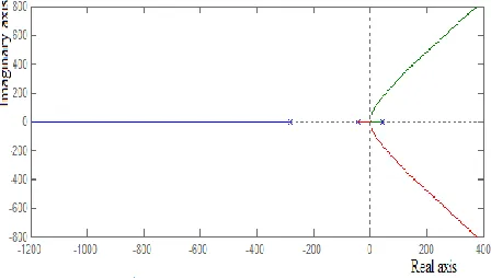
To verify whether simple gain adjustment will stabilize the system, a constant-gain compensator is used as shown in Fig. 5. The root locus for this situation is depicted in Fig. 6.
The root locus shows that no amount of increase in gain will result in system stability, as two of the system closed -loop poles always fall in the right-half s-plane. This is further supported by the Bode plot of the uncompensated system
(shown in Fig. 7), which clearly reveals that for any value of the system gain, both the gain margin and the phase margin remain negative. (See the appendix for a MATLAB script to create these plots.) Therefore, the most important design challenge here reduces to that of stabilizing the magnetic levitation system.
A. Proportional-Derivative Compensator
A general cascade proportional-derivative controller is described by the transfer function [9]
(25)
where Kp and KD are the proportional and derivative constants
of the controller, respectively.
Combining this with the maglev system transfer function results in the open-loop transfer function
(26)
To determine the ranges of values of Kp and KD that will
ensure system stability, the popular Routh-Hurwitz criterion [2] is used.
The system is stable if the condition
(27)
is met. The information given in (27) is used to generate root loci for the system in (26) in order to obtain an appropriat e combination of values of Kp and KD that guarantees stability
and gives good response. This is carried out by sweeping through various values for the ratio KP/KD and determining
proper corresponding values for Kp. The resulting loci are
displayed in Fig. 8.
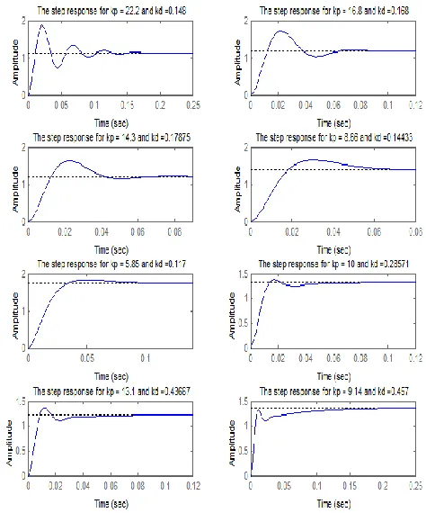
For the values of Kp/KD considered, Table I shows the
corresponding pairs of values of Kp and KD as well as the
closed-loop poles. The closed-loop responses are also shown in Fig. 9. From the responses, it is clear that the system can be stabilized by an appropriately designed PD compensator, although the system steady-state error is a bit high. It is important also to point out that the use of a proportional-derivative controller is limited in practice because of its inherent ability to amplify noise signals.
Sensor Compensator
Y
R V1
+ -
E UV2
G
s
Gs + -
G
c GMaglev system
Fig. 4. Overall closed-loop representation of the maglev system.
Y
R Kc
+
-
Fig. 5. Block diagram of a constant gain-compensated maglev system.
Fig. 7. T he bode plot of an uncompensated maglev system. Fig. 6. T he root -locus of a constant -gain compensated maglev
system.
s
p KD K 1 p K s D K p K E(s) U(s) ) s ( c G
551830 s
5 . 1946 2 s 50 . 283 3 s
s p KD K 1 p K 6 . 221457 )
s ( GH
50 . 283 D K p K ; 4918 . 2 p
Kp/KD Kp KD Pole s1 Poles s1, s2
150 22.2 0.148
0
-231.74 -25.88+134.77j, -25.88-134.77j
100 16.8 0.168
0
-185.51 -48.99+121.16j, -48.99-121.16j
80 14.3 0.178
8
-148.64 -67.43+114.22j, -67.43-114.22j
60 8.66 0.144
3
-137.38 -73.06+67.86j, -73.06-67.86j
50 5.85 0.117
0
-166.28 -58.61+32.21j, -58.61-32.21j
35 10 0.285
7
-31.09 -126.20+193.78j, -126.20-193.78j
30 13.1 0.436
7
-26.73 -128.39+267.23j, -128.39-267.23j
20 9.14 0.457
0
-15.48 -134.01+277.76j, -134.01-277.76j
B. Phase-Lead Compensator
As can be seen from the uncompensated maglev system root locus, a pair of a zero (located between s = 0 and s = - 44.1190) and a pole (located elsewhere in the right-half s-plane, but farther away to the left of the zero) can be used to augment the uncompensated open-loop transfer function of the maglev system in order to stabilize it. This gives rise to a phase-lead compensator. And a typical representation of a phase-lead compensator is given by [10]
b
a
;
b
s
a
s
c
K
)
s
(
c
G
(28)where Kc, a, and b are the compensator gain, zero, and pole,
respectively.
If (28) is used to compensate the maglev system, the resulting open-loop transfer function becomes
s
b
(s
3
283
.
50
s
2
1946
.
5
s
551830
)
a
s
c
K
6
.
221457
)
s
(
GH
(29)The root-contour approach can be employed to find the appropriate values of Kc, a, and b, or since an approximate
range of values of ‗b‘ is known, and the value of ‗a‘ can be deduced based on the reasoning that the farther ‗a‘ is from the imaginary axis (but not too close to the system open -loop pole at s = -44.1190) the better the stability, then the compensator parameters can be determined from root loci generated for varying values of Kc. The latter approach is used here.
Fig. 10 shows root loci for values of b between 44.119 and 490, and a = 35. From this fig., it is apparent that the greater the value of ‗b‘ the farther to the left the branches of the locus
Fig. 8. Root loci for pd-compensated maglev system various values of KP/KD.
TABLE I
SELECT ED PAIRS OF VALUES OF KP AND KD AND CORRESPONDING CLOSED-LOOP POLES
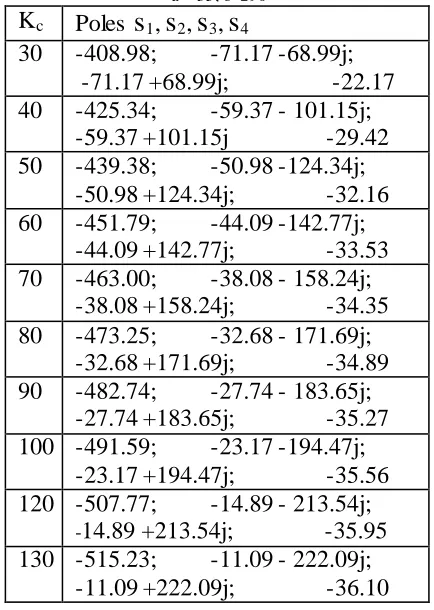
between s = -44.119 and s = -283.50 (or -b) are. And for a typical pair of a = 35 and b = 290, the range of values of Kc
that guarantees system stability is 24 < Kc < 212. For these
values of a and b, and a selected set of values of Kc, the
closed-loop poles are given in Table II while the closed-loop responses are displayed in Fig. 11.
K
cPoles
s
1,
s
2,
s
3,
s
430
-408.98; -71.17 -68.99j;
-71.17 +68.99j; -22.17
40
-425.34; -59.37 - 101.15j;
-59.37 +101.15j -29.42
50
-439.38; -50.98 -124.34j;
-50.98 +124.34j; -32.16
60
-451.79; -44.09 -142.77j;
-44.09 +142.77j; -33.53
70
-463.00; -38.08 - 158.24j;
-38.08 +158.24j; -34.35
80
-473.25; -32.68 - 171.69j;
-32.68 +171.69j; -34.89
90
-482.74; -27.74 - 183.65j;
-27.74 +183.65j; -35.27
100 -491.59; -23.17 -194.47j;
-23.17 +194.47j; -35.56
120 -507.77; -14.89 - 213.54j;
-
14.89 +213.54j; -35.95
130 -515.23; -11.09 - 222.09j;
-11.09 +222.09j; -36.10
TABLE IISelected values of Kc and the corresponding closed-loop poles for a = 35; b=290
CORRESPONDING CLOSED-LOOP POLES
Fig. 10. Root loci for a = 35 at various values of b.
IV. CONCLUSION
Stabilization of a magnetic levitation system has been the focus of this paper. Although the system is an unstable nonlinear one, it is clear that a linear compensator can be designed to stabilize it if its operation is limited to a small range (although this greatly limits the robustness of the compensator). We develop a complete nonlinear model of the system, and then form an approximate linearized equivalent from it. Based on this linearized model, we consider two linear compensators—proportional-derivative and phase lead—and show that the magnetic levitation s ystem can be stabilized by an appropriate selection of the parameters of the compensators using a classical design approach aided by a computer software tool. We compute and present the closed -loop poles of each design and the corresponding step responses, and also show the system stability limits. This approach proves quite useful and effective, as several simulation runs can be performed quickly to expedite the design. However, for a large-range operation, a more robust controller will be required to effectively bring the system into a region of stability. And for this latter type of controllers, several strategies, such as sliding mode control, adaptive control, etc., have been employed and are available in the literature, while the maglev system continues to attract more research attention.
APPENDIX
The various MATLAB scripts used in this tutorial are highlighted below.
A. Computation of the maglev system transfer function
% This script computes the transfer function of a maglev system using
% Y/U=C((SI-A)^-1)B.
syms s
% Define the parameters of the model.
R = 31.1; Lc = 0.1097; g = 9.81; K = 0.00065906; m = 0.01058;I = 0.125;
y0 = 0.01;
% Compute the values of A, B, and C.
A=[0 1 0;(2*K*I^2)/(m*y0^3) 0 (2*K*I)/(m*y0^2); 0 0 -R/Lc];B=[0 0 1/Lc]';
C=[1 0 0];
% Find the transfer function, Y/U.
id=eye(3,3);
disp('The transfer function is:') Tfunction=C*(inv(s*id-A))*B
% Find the simplified transfer function, Y/U.
[numTfunc,denTfunc]=numden(Tfunction);numTfunc=sy m2poly(numTfunc);
denTfunc=sym2poly(denTfunc);numTfunction=numTfun c/denTfunc(1);
denTfunction=denTfunc/denTfunc(1);
disp('While the simplified transfer function is now') tf(numTfunction,denTfunction)
B. The Root locus and bode plots of the uncompensate d maglev system
% This script plots the root locus and the bode diagram of the maglev
% system when compensated by a constant gain.
fnum=1419.6* 156;fden=[1 283.50 -1946.55 -551830]; sys1=tf(fnum,fden);
fig.(1) rlocus(sys1) fig.(2) bode(sys1)
C. The root loci for simulating the pd-compe nsate d maglev system
% Script for simulating the root locus -based pd-compensated design
kp_kd=[150 100 80 60 50 35 30 20]; L=length(kp_kd);
sysden=[1 283.50 -1946.5 -551830]; i=1;
while(i<=L) f=kp_kd(i);
sysnum=221457.6*[0 0 1/f 1]; subplot(4,2,i)
rlocus(sysnum, sysden)
str=['The root locus for kp / kD = ' num2str(f)]; title(str)
axis([-150 50 -200 200]); i=i+1;
end
D. Closed-loop poles and step responses of the pd-compensated maglev system
% Script for generating the closed-loop poles as well as the responses of
% the pd-compensated maglev system.
kp_kd=[150 100 80 60 50 35 30 20]; kp=[22.2 16.8 14.3 8.66 5.85 10 13.1 9.14]; kd=kp./kp_kd;
L=length(kp_kd);
sysden=[1 283.50 -1946.5 -551830]; sys2=1;syspoles=zeros(8,3); i=1;
while(i<=L)
f1=kp_kd(i);f2=kp(i);
sysnum=f2*221457.6* [0 0 1/f1 1]; sys1=tf(sysnum,sysden);
sysfun=feedback(sys1,sys2); syspole=eig(ss(sysfun))'; syspoles(i,1:3)=syspole; subplot(4,2,i)
step(sysfun)
str=['The step response for kp = ' num2str(f2) ' and kd ='...
num2str(f1)]; title(str) i=i+1;
end
disp('The closed-loop poles are:') syspoles;
E. The root loci for simulating the phase lead-compensated maglev system
% Script for simulating the root locus -based phase lead-compensated design.
sysnum=221457.6*[0 0 0 1 a]; sysden1=[1 283.50 -1946.5 -551830];
b=[50 100 150 200 250 290 340 390 440 490]; Lb=length(b);
i=1;clf;
while(i<=Lb) f1=b(i);
sysden=conv([1 f1],sysden1); fig.(3)
subplot(5,2,i)
rlocus(sysnum, sysden)
str=['The root locus for a = ' num2str(a) ' and b = '
num2str(f1)]; title(str)
axis([-200 100 -200 200]) i=i+1;
end
F. Closed-loop poles and step responses of the phase lead-compensated maglev system
% Script for generating the closed-loop poles as well as the responses of
% the pase lead-compensated maglev system when b = 290.
a=37.5; b=290;
kc=[30 40 50 60 70 80 90 100 120 130]; L=length(kc);
sys2=1;syspoles=zeros(10,4); i=1;
while(i<=L) f1=kc(i);
sysnum=f1*221457.6* [0 0 0 1 a];
sysden=conv([1 b],[1 283.50 -1946.5 -551830]); sys1=tf(sysnum,sysden);
sysfun=feedback(sys1,sys2); syspole=eig(ss(sysfun))'; syspoles(i,1:4)=syspole; fig.(5)
subplot(5,2,i) step(sysfun)
str=['The step response for a = ' num2str(a)' , b = '
num2str(b)',...
and kc = ' num2str(f1)]; title(str)
i=i+1;
end
disp('The closed-loop poles are:') syspoles
REFERENCES
[1] Franklin G.F., Powell J.D., and Workman M., Digital Control of Dynamic Systems, Addison Wesley Longman, Inc., 1998, pg. 273. [2] Nise N. S., Control Systems Engineering, Wiley India (P.) Ltd., Delhi,
T hird Reprint, 2007, pp. 329-352.
[3] Naumivic M. B., Veselic B. R., ―Magnetic levitation system in control engineering education,‖ Automatic Control and Robotics, vol. 7, no.1, 2008, pp. 151-160.
[4] Green S.A., Hirsch R.S., and Craig K.C., ―Magnetic levitation device as teaching aid for mechatronics at Rensselaer,‖ Proc. ASME Dynamic Systems and Control Division, vol. 57-2, 1995, pp. 1047–1052. [5] Feedback Instrument Limited, Magnetic levitation system —getting
started, http://www.fdb.com, 18th September, 2012.
[6] Al-Muthairi N. F., and Zribi M., ― Sliding mode control of a magnetic levitation system,‖
Mathematical Problems in Engineering 2004, vol. 2, 2004, pp. 93 -107. [7] Kuo B. C., and Golnaraghi F., Automatic Control Systems, John Wiley &
Sons (Asia) Pte. Ltd., 2003, pp. 110 -111.
[8] Shahian B., and Hassul M., Control System Design Using MAT LAB. Englewood Cliffs: Prentice Hall, 1993, pp. 455 –465.
[9] Katsuhiko O., Modern Control Engineering, Prentice Hall of India Private Ltd., New Delhi, T hird Edition, 2000, pg. 216.
[10] Richard C.D., Robert H.B., Modern Control Systems, Pearson Education (Singapore) Pte. Ltd., Indian Branch, Delhi, First Indian Reprint, 2004, pg. 566.
Ayokunle A. AWELEWA graduated with a Bachelor of Engineering degree in Electrical Engineering from University of Ilorin, Ilorin, Kwara State, Nigeria, in 2001, and a Master of Engineering degree (electric power & machine) from Covenant University ,where he is currently a lecturer in the Department of Electrical & Information Engineering, Ota, Nigeria, in 2007. His research areas include power system stabilization and control, and modeling and simulation of dynamical systems.
Isaac A. SAMUEL obtained a postgraduate diploma and a Master of Engineering degree in Electrical/Electronics Engineering from Bayero University, Kano, Nigeria, in 2003 and 2006, respectively. He is currently a lecturer in the Department of Electrical & Information Engineering, Covenant University, Ota, Nigeria. His research areas include power system operation, reliability, and maintenance.