International Journal of Mechanical & Mechatronics Engineering IJMME-IJENS Vol:14 No:06 93
148506-1919-IJMME-IJENS © December 2014 IJENS
Implementation of Gain Scheduled PID Controller for
a Nonlinear Coupled Spherical Tank Process.
1
D.Pradeepkannan
, 1Associate Professor, Electronics and Instrumentation Department, K.L.N College of Engineering, Pottapalayam,TamilNadu, India. [email protected]
2
Dr.S.Sathiyamoorthy
2 Professor, Electronics and Instrumentation Department, J.J. College of Engineering and Technology, Trichy, Tamilnadu India.
Abstract- Conventional PID controller is a simplest known
controller used in almost all process Industries for controlling the process parameters at desired set value. As the dynamics of a coupled interacting spherical tank process is highly nonlinear, it exhibits non linear behaviour and time delays between the inputs and outputs, The ZN tuned PID controller parameters does not adapt with all operating points as it exhibits different non linear characteristics. The aim of this proposed work is that real time implementation of Gain scheduled PID controller to enhance the performance of the conventional PID controller of a nonlinear coupled interacting spherical tank process. A gain scheduler which fine tunes and schedules the controller parameters based on the instantaneous value of the process variable so as to adapt with all operating points. The controller performance of the ZN tuned PID controller and gain scheduled PID controller are compared in terms of time domain specification as well as performance indices. Better enhanced controller performance was obtained for a Gain scheduled PID controller than that of ZN tuned PID controller at all operating points. The real time implementation is done on a coupled spherical tank setup in LabVIEW Environment using NI compact –RIO, an inbuilt FPGA control hardware.
IndexTerm—Gain Scheduling, LabVIEW, PID controller,
Spherical Tank Process, ZN Tuning,
1. INTRODUCTION
Proportional Integral Derivative Controller has been using in Industrial control applications for a long time. The reasons for their wide popularity lies in the simplicity of design and good performance which includes low percent over shoot and small settling time for slow process Astrom.K.J and Hagglund.T,(1995).According to the survey in 1989, 90% of process industries uses the conventional PID controllers [3].The wide spread use of the PID controller in the Industry is due to their simplicity and ease of retuning online feature of PID controller. [4-7].The PID controller is so named because its output sum of three terms, Proportional, Integral and Derivative term. Each of these terms is dependent on the error value ‘e’ between the input and the output.
0
1
tc d
i
de( t )
u( t )
K [ e( t )
e( t )dt
]
dt
[1] e(t) is the error signal, u(t) is the controller output, Kc is thecontroller gain, τi and τd are integral gain and derivative gain.
Proportional term speeds up the response as the closed loop time constant decreases with the proportional term but does not change the order of the system as the output is just proportional to the input. The proportional term minimizes but does not eliminate the offset .Integral term eliminates the offset as it increases the type and order of the system by one. This term also increases the system response speed but at the cost of sustained oscillations. Derivative term primarily reduces the oscillatory response of the system. It neither changes the type and order of the system nor affects the offset. Determining
optimum value of Proportional constants kp,i,d is termed as
tuning. Any change in these parameters cause changes in the type, order and response of the system. Thus they play a vital role in obtaining a good controller performance characteristics. There have been a various types of tuning techniques applied for PID controller. One of the oldest is that Ziegler Nichols Tuning. These techniques may be of Optimization technique or classical technique. Classical techniques make certain assumptions about the plant and the desired output and try to obtain analytically, or graphically some feature of the process that is then used to decide the controller settings. These techniques are computationally very fast and simple to implement, and are good as a first iteration. But due to the assumptions made, the controller settings usually do not adapt with non linear behavior of the process and are unable to give desired response at all operating points which then requires further fine tuning. The Ziegler and Nichols first PID tuning method is the techniques made based on certain controller assumptions. Hence, there is always a requirement of further tuning. Further the controller settings derived are rather aggressive and thus result in excessive overshoot and oscillatory response. Also the controller parameters are rather difficult to estimate in noisy environment. The second method is based on knowledge of the response to specific frequencies. The idea is that the controller settings can be based on the most critical frequency points for stability. This method is based on experimentally determining the point of marginal stability. This frequency can be found by increasing the proportional gain of the controller, until the process becomes marginally stable. The gain is called ultimate gain Ku and the time period Tp. These two parameters define one point in the Nyquist plots.
The process exhibits non linear behavior at various operating points, this work aims at designing a gain scheduled controller and there by fine tuning of the controller settings so as to obtain an enhanced control performance at all operating points. This paper is organized as follows. The section 1 gives a brief introduction of the work. The section 2 provides a brief review of Gain scheduled controller. Section 3 explains about the mathematical modelling of the non-linear spherical tank process. Section 4 describes the Experimental set up and its real time implementation of conventional PID controller and Gain scheduled PID controller. Section 5 describes the Results obtained for servo operation and servo regulatory operation at various operating points of the tank for both ZN PID controller and Gain scheduled PID controller. Finally the conclusion is given in section 6.
2. GAIN SCHEDULED CONTROLLER
148506-1919-IJMME-IJENS © December 2014 IJENS I J E N S
nonlinearities. It is then possible to change the parameters of the controller by monitoring the operating conditions of the process. This idea is called gain scheduling, since the scheme was originally used to accommodate changes in process gain only. Gain scheduling is easy to implement in computer-controlled systems, provided that there is support in the available software. Gain scheduling based on measurements of operations of the process is a good way to compensate for variations in process parameters or known nonlinearities of the process. If we use the informal definition of adaptive controller, Gain scheduling is a very useful technique for reducing the effects of parameter variations. There are also many commercial process control systems in which gain scheduling can be used to compensate for static and dynamic nonlinearities. Split-range controllers that use different sets of parameters for different ranges of the process output can be regarded as a special type of gain-scheduling controllers. It is sometimes possible to find auxiliary variables that correlate well with the changes in process dynamics. It is then possible to reduce the effects of parameter variations simply by changing the parameters of the controller as functions of the auxiliary variables. Gain scheduling can thus be viewed as a feedback control system in which the feedback gains are adjusted by using feed forward compensation. A main problem in the design of systems with gain scheduling is to find suitable scheduling variables. This is normally done on the basis of knowledge of the physics of the systems.
Fig. 1. Schematic diagram of Gain scheduled Controller
When scheduling variables are determined, the controller parameters are calculated at a number of operating conditions by using some suitable design method. The controller is thus tuned or calibrated for each operating condition. The stability and performance of the system are typically evaluated by simulation.
3. MATHEMATICAL MODELLING
Consider the coupled Interacting spherical tank process shown in Figure 2. The objective of the process is to control the level of the two tanks namely ha(t) and hb(t).
Fig. 2. Schematic diagram of Coupled Interacting Spherical tank Process
The inlet water flow from the two pumps f1 (t) and f2 (t) are
used as manipulated variables so as to keep the control variable at the desired set point. The level of the tank at any instant is measured by the combination of orifice and Differential pressure transmitters which are mounted on the respective tanks discharge line whose output is (4 -20)mA. This output are compared with the desired set point value of level one and level two which will be configured as (4 -20)mA. The error signal is amplified based on the controller specification. The controller outputs is used to vary the inflow rates f1(t) and f2(t)
of the spherical tank so as to maintain the set point at desired level ha and hb of the tanks. Electro pneumatic converters are
used to convert the controller outputs of (4 -20)mA in to a pneumatic signal of (3-15) psi so that the final control element will be able to throttle the inflow rates f1 and f2. Using the law
of Conservation of mass, the non linear plant equations are obtained.
For tank 1, f1 - f 3 – f4 = (Ah) dha/dt [2]
For tank 2, f3 +f 2 – f5 = (Ah) dhb/dt [3]
Where, f1 and f2 are in flow rates to tank1 and tank2 respectively
in (m3/sec).
f4 and f5 are outflow rate of tank 1 and tank 2 (m3/sec).
f3 flow rate between the tanks (m3/sec).
Radius on the surface of the fluid varies according to the surface level of fluid in the tank. Let this radius be known
as
r
s.Therefore rs12=√2raha – ha2 and rs22 = √2rbhb – hb2Where ra= radius of tank1 in metres.
rb= radius of tank2 in metres.
ra= rb= r =0.5metres
ha = fluid level in tank1 in metres.
hb = fluid level in tank2 in metres.
x 0 = thickness of pipe 0.04 in metres.
f 3 = a √2g(ha – hb ) [4]
f 4 = a√2g(ha - x0 ) [5]
f 5 = a√2g(hb - x0 ) [6]
Where a=π[x0 /2] 2
has - steady state water level of tank 1 in metre.
hbs - steady state water level of tank 2 in metre.
As the dynamics of the spherical tank is non linear in nature, the controllable height (0-45) centimetres of the tank is divided in to three regions such as (0-15)cm as region1,(16-30)cm as region2 and (31-45) as region3.
The linearised plant transfer function for region 1 at a set point of 0.1metre for tank1 and 0.09metre for tank2 in S domain are
given as 2
11
3 573 0 2876
0 1512 0 0023
. s .
( s )
s . s .
G
[7]2 22
3 888 0 2749
0 1512 0 0023
. s .
( s )
s . s .
G
[8]2 21
0 2473 0 1512 0 0023
. ( s )
s . s .
G
[9]2 12
0 1917
1512 0023
. ( s )
s . s .
G
[10] The linearised plant transfer function for region 2 at a set pointof 0.22metre for tank1 and 0.21metre for tank2 in S domain are
given as
2 11
1 855 0 0881
0 0794 0 0008
. s .
( s )
s . s .
G
[11]2 22
1 919 0 0612
0 0794 0 0008
. s .
( s )
s . s .
G
[12]2 21
0 0489
0 0794 0 0008 .
( s )
s . s .
G
[13]O/P CONTROLLER PROCESS
OPERATING CONDITIONS
International Journal of Mechanical & Mechatronics Engineering IJMME-IJENS Vol:14 No:06 95
148506-1919-IJMME-IJENS © December 2014 IJENS 2
12
0 0492 0794 0008
. ( s )
s . s .
G
[14] The linearised plant transfer function for region 3 at a set pointof 0.36metre for tank1 and 0.35metre for tank2 in S domain are given as in S domain are given as
2 11
1 34 0 0307
0 0447 0 0001
. s .
( s )
s . s .
G
[15]2 22
1 399 0 0305
0 0477 0 0001
. s .
( s )
s . s .
G
[16]2 21
0 0259 0 0477 0 0001
. ( s )
s . s .
G
[17]2 12 0 026 0447 0001 . ( s )
s . s .
G
[18]3.1 Black box modeling
Consider the first order system with dead time represented by the following transfer function
1 d t s p p k e G( s )
s
[19] The output response to a step change in input is given by,
p 1 py( t ) k u( exp( ( t ) / )) for t> [20]
The measured output is in deviation variable form. The three process parameters K ,p p, can be estimated by performing a
single step test on process input. The process gain is found as simply the long term change in process output to the change in process input. The time delay is the amount of time, after the input change, before a significant output response is observed.
3.2 Estimation of time constant by two point method
Smith has obtained the parameters of FOPDT transfer function model by letting the response of actual system and that of the model to meet the two points which describe the parameter &
p td
. Here, times required for the process output to make 28.3% and 63.2% respectively are measured. The time constant and time delay can be estimated from the equation given below for both the transfer function,
2 3 3
3 0 4 0 7
p ( t / ) ( t / ),td t / . p
. [21]
Thus the obtained FOPDT models for various regions are determined and shown in the table I.
Table I Tank1 operating point in metres Tank 2 operating point in metres FOPDT Model for tank1 FOPDT Model for tank2
0.1 0.09 123 75 2 648
52 87 1
. s . e . s 5 33 119 5 54 62 1
. s
. e
. s
0.22 0.21 4 492
110
81 58 1
. s e . s 8 79 76 425
70 72 1
. s
. e
. s
0.36 0.35 15 78
306 48 409 7 1
. s . e . s 23 61 304 73 422 833 1
. s . e . s
The parameters of the controllers as per Ziegler Nichols tuning method are found by applying Bode stability criterion, the phase cross over frequency is determined and the amplitude
ratio is equate to unity at phase cross over frequency
w
p whenthe system is on the verge of instability. Thus by equating
( ) 1
p
G jw w w= = the ultimate gain Kcu is determined. The
ultimate period Pu is defined as the period of the sustained
cyclic that would occur if a proportional controller with a gain Kcu where used and
p
u=2
p w
p The Ziegler Nichols setting forcontrollers are determined directly from Kcu and Pu according
to the rule summarized in the table II.
TableII
Controller Type
c
k
t
it
dP 0.5 Kcu - -
PI 0.45 Kcu Pu/1.2 -
PID 0.6 Kcu Pu/2 Pu/8
Applying the Ziegler Nichols tuning rules for various regions of the tanks FOPDT models, the corresponding controller setting are determined and shown in the table III and table IV.
Table III
Tank1
operating point in metres
ZN PID controller tuning values for tank1
Kp Ki Kd
0.1 0.1538 0.029 0.2013
0.22 0.1602 0.031 0.21
0.36 0.1058 0.0064 0.4372
Table IV
Tank 2operating point in metres
ZN PID controller tuning values for tank2
Kp Ki Kd
0.09 0.0851 0.0084 0.2156
0.21 0.1058 0.0064 0.4372
0.35 0.0583 0.0013 0.654
3.3 Decoupler design
The effect of interactions in a MIMO system is minimized with the introduction of decoupler. Thus for the coupled non linear interacting spherical tank system, the decoupler are designed for all the three regional transfer functional models and shown in table V.
Table V Tank1 operating point in metres Tank 2 Operating point in metres FOPDT Model for tank1 FOPDT Model for tank2
0.1 0.09 0 1917
3 573 0 2876
.
. s .
0 2473
3 888 0 2749
.
. s .
0.22 0.21 0 0492
1 8550 0 0881
.
. s .
0 0489
1 919 0 0612
. . s .
0.36 0.35 0 026
1 34 0 0307
.
. s .
0 0259
1 399 0 0305
. . s .
3.4 Model validation
148506-1919-IJMME-IJENS © December 2014 IJENS I J E N S
0 10 20 30 40 50 60 70
0 20 40 60 80
Time in seconds
H
e
i
g
h
t
o
f
t
h
e
t
a
n
k
i
n
c
m
s
Open loop response of two interacting process foe a given unit step changein set point
open loop response of process for tank1 open loop response of process for tank 2 open loop response of FOPDT model for tank1 open loop response of FOPDT model for tank 2 Unit Step input
Unit step input
Fig. 3. Open loop response of actual transfer function and FOPDT model of tank1
It is evident from the figure 3 that both the responses coincides and have similar time domain response. Hence FOPDT model approximation can be used for tuning the PID controller to obtain optimal values of controller parameters.
4. IMPLEMENTATIONOFGAINSCHEDULEDPID
CONTROLLER
The experimental set up of the coupled spherical tank system is made up of SS316 material which has high corrosion resistance property and has a maximum height and radius of 0.5 meter. Water from the reservoir tank of size 1250mm x 450mm x 450mm is pumped through a Kirloskar make 0.5 HP pump having a discharge of 1500 litres per hour that flows through a rotameter having a range of (40 - 440) LPH to the spherical tank. The level of the tank at any instant is measured by the Rose mount Differential pressure transmitter having a measurement range of (0-400)mm of water column corresponds to the output range of (4 -20)mA. This output is compared with the desired set value of level which will be scaled in the control law as (4 -20)mA. The error signal is also in the range of (4-20)mA which is then amplified based on the controller specifications.
Fig. 4. Experimental set up for coupled interacting spherical tank system
Fig. 5. real time FPGA control hardware CRIO 9025/9215
This output is used to vary the inflow rate q1(t) of the spherical
tank with the use of an ABB make Electro pneumatic converter which converts the output of (4 -20)mA in to a pneumatic
signal of (3-15) psi so that the Equal percentage control valve will be able to throttle the inflow rate. The controller parameters are determined for both ZN tuned PID Controller as well as Gain scheduled PID controllers. The values of kp, ki, kd
for ZN tuned PID are found to be 0.33, 0.036, 0.7623 respectively. A real time in built FPGA control hardware from National Instrument c-RIO 9025 is use to communicate the data from the transmitters to the PID controller block of Lab VIEW program both for ZN and Gain scheduled PID control. The response for a given step change in inflow rate qi, and the
corresponding steady state response is obtained as illustrated in the results. To implement the gain scheduled PID controller, the determined gains of three regions are fed to the lab VIEW gain scheduler block which in turn schedules the PID gain values based on the instantaneous gain scheduler variable and the corresponding servo, regulatory, and the servo regulatory response are obtained and as shown in the results .
5. RESULTS AND DISCUSSION
A step response of Gain scheduled PID controller are obtained for servo problem and servo regulatory problem and their performance characteristics are compared in terms of time domain specifications such as rise time, peak time, peak over shoot, steady state value etc and performance indices such as ISE and IAE.
0 50 100 150 200 250 300 350 400 0
10 20 30 40 50
Time in seconds
S
e
t
p
o
in
t
a
n
d
p
r
o
c
e
s
s
v
a
r
ia
b
le
in
c
m
s
Servo response of Gain Scheduled PID Controller
Region 3 response of tank2 Region 3 response of tank1 Region1 set point of tank1 in cms Region 1 set point of tank2 in cms Region 2 response of tank1 Region 2 set point of tank1 in cms Region 2 response of tank1 Region 2 set point of tank2 in cms Region 3 set point of tank1 in cms Region 1 response of tank2 Region 3 set point of tank1 Region 1 response of tank2.
Fig.6. Servo response of Gain scheduled PID Controller for various set points
It is evident from the above response that Gain scheduled PID controller could track the set points with minimal settling time and with lesser over shoot for various operating points.
0 100 200 300 400 500 600
5 10 15 20 25 30 35 40
Time in seconds
S
e
t
p
o
in
t
a
n
d
p
r
o
c
e
s
s
v
a
r
ia
b
le
i
n
c
m
s
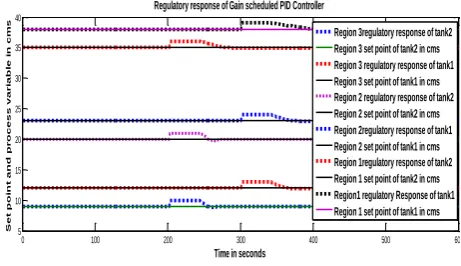
Regulatory response of Gain scheduled PID Controller
Region 3regulatory response of tank2 Region 3 set point of tank2 in cms Region 3 regulatory response of tank1 Region 3 set point of tank1 in cms Region 2 regulatory response of tank2 Region 2 set point of tank2 in cms Region 2regulatory response of tank1 Region 2 set point of tank1 in cms Region 1regulatory response of tank2 Region 1 set point of tank2 in cms Region1 regulatory Response of tank1 Region 1 set point of tank1 in cms
Fig. 7. Regulatory response of Gain scheduled PID Controller for various operating points
International Journal of Mechanical & Mechatronics Engineering IJMME-IJENS Vol:14 No:06 97
148506-1919-IJMME-IJENS © December 2014 IJENS Fig. 8. Response of Gain scheduled PID controller for a set point of 18 and 8
cms of water column with 30 samples per second.
It is evident from the response that the Gain scheduled PID controller output could track the set point at a different operating points such as 18cms and 8cms of water column for both the tanks with a nominal settling time and with minimal overshoots.
Fig. 9. Response of gain scheduled PID controller for a set point of 29cms of water column with sampling rate T=30 samples per seconds.
It is evident from the response that the gain scheduled PID controller output could track the set point at a different operating point of 29cms of water column with a settling time of 95.2 and 95 seconds and with18.09% and 13.08% overshoots.
Fig. 10. Response of gain scheduled PID controller for a set point of 35cms of water column with sampling rate T=30 samples per seconds.
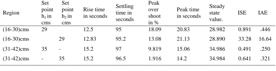
Table IV
shows the servo response at various operating points with time domain specification of Gain Scheduled PID controllers against conventional PID controller at various height of the spherical tank.
Region
Set point h1 in
cms Set point h2 in
cms
Rise time in seconds
Settling time in seconds
Peak over shoot in %
Peak time in seconds
Steady state value.
ISE IAE
(16-30)cms 29 12.5 95 18.09 20.83 28.982 0.891 .446
(16-30)cms 29 12.83 95.2 13.08 21.13 28.890 33.28 16.64
(31-42)cms 35 - 15.2 97 9.819 15.06 34.986 0.491 .250
(31-42)cms - 35 15.2 96.5 1.916 14.2 34.984 0.641 .321
It is evident from the response that the Gain scheduled PID controller output could track the set point at a different operating point of 35cms of water column with a settling time of 97 seconds for tank1 and 96.5 seconds for tank2 respectively and with a smooth response of very little overshoots. The Gain Scheduled PID controller output could track the set point at a different operating points such as of 29 and 35 cms of water column for both the tank1 and tank2 with a settling time of 95,95.2 and 96.5,97seconds and with minimal overshoot respectively. A step response of Gain scheduled PID controller for various regions of the tank are obtained for servo problem and servo regulatory problem and their performance characteristics are compared in terms of time domain specifications such as rise time, peak time, peak over shoot, steady state value etc and performance indices such as ISE and IAE.
6. CONCLUSION
148506-1919-IJMME-IJENS © December 2014 IJENS I J E N S
ACKNOWLEDGEMENT
This work was supported by department of Electronics & Instrumentation Engineering and Research & Development unit of K.L.N. College of Engineering, Pottapalayam, Sivagangai district, Tamilnadu, India.
REFERENCES
[1] AnandanatarajanR. Chidambaram.M and Jeyasingh T,”Limitations
of PI Conroller for a first order nonlinear Process with Dead Time”,ISA Transactions, Vol 45.pp. 185-200.2006.
[2] Astrom K.J. and T. Hagglund,” Automatic Tuning of Simple
regulators with specifications on Phase and Amplitude margins”,Automatica Vol 20, no. 5,pp 645-651,1984.
[3] AstromK.J.andT.Hagglund,”PID controllers, Theory, design and
tuning”, 2nd edition”, Instrument Society of America, 1995.
[4] Astrom K.J.and T. Hagglund,” The Future of PID Control”,
Control Engineering Practice,Vol 9, 2001pp 1163-1175.
[5] AstromK.J.,T.Hagglund, C.C.Hang, W.K.Ho, “Automatic Control
and Adaptation for PID Controllers - A Survey,”Control Engineering Practice ,Vol1, no 4,PP 699-714,1993.
[6] Bhuvaneswari N.S. and Kanagasabapathy P.(1998),”Studies on
time optimal control of tank level’,Proceedings of national conference on role of fuzzy logic ,neural networks and genetic algotithm in process control’, pp. 48-55.
[7] Bhuvaneswari,N.S.,UmaG.and RengaswamyT.R.,”Neuro based
Model reference adaptive controlof a conical tank level process”,Journal of control and Intelligent System’,36(1),pp.98-106.
[8] Hagglund T. and K.J Astrom, “Industrial Adaptive Controllers
Based on Frequency Response Techniques,” Automatica, vol. 27,
no. 4, pp. 599-609, 1991.
[9] Nithya.S, G.Abaysingh, N.Sivakumaran, T.K.RadhaKrishnan,
T.Balasubramanian and N.Anandaraman.,”Design of Intelligent
Controllers for Nonlinear processes”Asian Journal of Applied Sciences.,1.pp33-45.
[10] Nithya.S,N.Sivakumaran,T.K.RadhaKrishnan, T.Balasubramanian
and N.Anandaraman.,”Model based controller design for a
spherical tank process in real time”,IJSSST,vol 9,No.4,pp 25-31,2008.
[11] PradeepKannan.D, and S.Sathiyamoorthy,” Design and Modelling
of State Feedback with Intergal Controller for a Non-Linear spherical tank Process”, International Journal of Emerging
Technology and Advanced Engineering, 2(11),.668-672,2012.
[12] Ravi.V. and R.Thyagarajan T.,”A decentralized PID Controller
for Interacting nonlinear systems”,Proceedings of Emerging trends in Electrical and Computer Technology, pp 297-302, 2008.
[13] Weng Khuen Ho, Chang Chieh Hang, Lisheng S.Cao, “Tuning of
PID Controllers Based on Gain and Phase Margin Specifications” Automatica Vol 31,no.3,PP 497-502, 1995.
Bibliography
D.Pradeep kannan received his Bachelors Degree in Instrumentation and Control Engineering from Madurai Kamaraj University, India. in 1999 and Master degree in Industrial Engineering in 2001 from Madurai kamaraj University..Currently he is an Associate professor in the department of Electronics and Instrumentation Engineering in K.L.N. College of Engineering, Madurai, India. He is pursuing his Research program at Anna University Chennai India. He has published about 4 papers in reputed Journals and Conferences. His research interests includes Process Control, Fraction order PID controllers, Tuning of controllers for nonlinear processes using soft computing techniques etc. He is a life member of ISTE and ISOI societial bodies. His mail id is [email protected].
Dr.S.Sathiyamoorthy, Principal of J.J. College of Engineering and Technology has sixteen years of experience in Teaching, Research and Industry. He has completed B.E. Degree in Electrical and Electronics
Engineering, Regional Engineering
College, Tiruchirapalli in 1995, and M.E. degree in Control and Instrumentation at
Guindy Engineering College, Anna
University, Chennai in 2002. He has received his Doctorate from National Institute of Technology, Tiruchirapalli in 2008. He has
organised many National, International conferences and
workshops. He has published several papers in leading International journals. He has given numerous expert lectures in various forums and Colleges in area of Neural Networks and Fuzzy logic control. His areas of specialization are Process Control and Industry Automation, Multiphase flow identification using
Electrical Capacitance Tomography. His mail id is