Volume 1, Issue 10 (November2012) PP: 35-42
Passive Force on Retaining Wall Supporting Φ Backfill
Considering Curvilinear Rupture Surface
Sima Ghosh
1*, Nabanita Datta
21Civil Engineering Department, National Institute of Technology, Agartala, PIN-799055 2
Civil Engineering Department, National Institute of Technology, Agartala, PIN-799055
Abstract:––The passive resistance of retaining walls denotes the stability of the wall against failure. Most of the available methods for calculating the passive earth pressure are based on linear failure surface. In this paper, the expression of seismic passive earth pressure acting on inclined rigid retaining wall is derived considering the non-linear failure surface. The Horizontal Slices Method with limit equilibrium technique has been adopted to establish the nonlinearity of rupture surface. Detailed discussion of results with variation of several parameters like angle of internal friction (Φ), angle of wall friction (δ), wall inclination angle (α) and surcharge loading (q) have been conducted.
Keywords:––Active earth pressure, Passive earth pressure, Φ backfill, rigid retaining wall, wall inclination, curvilinear rupture surface.
I.
INTRODUCTION
The lateral earth pressure is generally a function of the soil properties, the wall and the intensity of loadings acting on the wall. Earth pressure theories constitute one of the most important parts in the Geotechnical structures. Coulomb (1776) was the first to establish the formulation for Active and Passive earth pressure for the retaining structures. Rankine‟s theory (1857) has given a general solution for determination of passive earth pressure. Graphical methods have also been established by Culmann (1865). The analyses have been conducted considering the Φ nature of backfill. The calculations are based on Limit equilibrium technique. In most of the cases, the researchers have assumed the failure surface to be linear. In practical condition, the failure surface may not be linear. In this particular analysis, the failure surface has been assumed to be non-linear and Horizontal Slice Method has been taken into consideration to calculate the optimum value of passive earth pressure acting on each slice. Generalized equation has been established to find the solution for „n‟ number of slices.
II.
METHOD OF ANALYSIS
The analysis has been made in the same way as in the case of active earth pressure. The line of action of Pp and R
is acting from the upward direction. The slicing and other analysis are the same. Details may be seen in the Figures 1 and 2. The forces acting on the wall has been calculated by considering the following parameters:
Hi-1, Hi = Horizontal shear acting on the top and bottom of the ith slice.
Wi = Weight of the failure wedge for ith slice.
Vi-1,Vi = Vertical load (UDL) on top and bottom of i th
slice. Φ = The angle of internal friction of soil.
Ppi = Passive earth pressure on i th
slice.
Ri = The reaction of the retained soil on ith slice.
δ = The angle of wall friction.
III.
DERIVATION OF VARIOUS FORMULATIONS DURING THE PASSIVE CASE OF
EQUILIBRIUM
Applying the force equilibrium condition, we can solve the equations in the following pattern
))
)
1
(
tan(
(tan
)
(
)
2
1
(
)
)
1
(
sin(
)
sin(
1 2 1 r r i ii
i
i
R
P
(6)Solving these two equations, we find the value of generalized equation for Passive earth pressure for ith slice as follows:
)
)
1
(
sin(
)}
)
1
(
sin(
))
tan
)
)
1
(
)(tan(
1
(
tan
)
(
)}
{tan(
tan
2
))
)
1
(
cos(
))(
)
1
(
tan(
)(tan
1
2
{(
)
(
2
1 1 1 1 1 1 1 2 r r r n i m r r r i pi
i
i
i
i
n
m
i
i
i
P
Where,
tan(
1
m
r)
0
for i = n (7) The passive earth pressure coefficient can be simplified as,2 1
2
n i pi pP
K
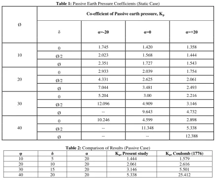
(8) Optimization of the passive earth pressure coefficient Kip is done for the variables θ1 and a satisfying the optimization criteria. The optimum value of Kip is given in Table 1.IV.
PARAMETRIC STUDY
A detailed Parametric study has been conducted to find the of variations of static passive earth pressure with
various other parameters like soil friction angle (Φ), wall inclination (α), wall friction angle (δ). For Φ = 100, 200, 300, 400
and δ = 0, Φ/2, Φ and α = +200, 0, -20⁰
Fig.1 Inclined Retaining Wall (Passive state of equilibrium)
Ѳ
nα
Ø
R
W
δ
P
pH
Ѳ
1+Ѳ
Fig.2 Detailed drawing showing various components of the retaining wall along with slices (passive state of equilibrium). The details of these studies are presented below:
4.1 Effect of Inclination of the wall (α)
Fig.3 to 5 represents the effect of inclination of the wall on the passive earth pressure for different value of δ. From these Figures, it is seen that due to increase in α, passive earth pressure is going to be decreased. The reason behind it is that when the inclination of the wall is positive with the vertical then the passive resistance acting on the wall is less compared to the wall inclined negative with the vertical. For example at Φ = 10° and δ =0°, the decrease in Kp is 4.4% for α = +20° over α
= 0 value, where as the increase in Kp is 22.8% over α = 0 value for α = -20. Again at Φ = 20° and δ = Φ /2, the decrease in
Kp is 21.5% for α = +20° over α = 0 value, where as the increase in Kp is 65% over α = 0 value for α = -20. Again at Φ = 20°
and δ = Φ, the decrease in Kp is 28.3% for α = +20° over α = 0 value, where as the decrease in Kp is 102.4% over α = 0 value
for α = -20. It is also observed that the value of Kp for α = -20° and δ = Φ, increases with the increase in the value of Φ upto
Φ = 20.
ΔH
V
1H
1Ø
δ
R
1P
1α
W1
ΔH
Ѳ
1V
n-1H
n-1Ø
δ
R
nP
nα
Wn ѲnV
i-1V
iH
i-1H
iØ
R
iP
iα
Wi
Ѳ1+(i-1)ѲR
LAYER - 1
LAYER - n
LAYER - i
ΔH
1.2
Effect of Wall Friction Angle (δ)Fig.6 to 8 represents the effect of wall friction angle on the passive earth pressure for different value of α. From these Figures, it is seen that due to increase in δ, passive pressure is going to be increased. The reason behind it is that the frictional resistance between wall and soil is increasing with the increase in the value of δ. For example at Φ = 10° and α =20°, the increase in Kp is 6.3% for δ = Φ/2 over δ = 0 value, where as the increase in Kp is 13.6% for δ = Φ over δ = 0.
Again at Φ = 20° and α =0, the increase in Kp is 28.7% for δ = Φ/2 over δ = 0 value, where as the increase in Kp is 70.7% for
δ = Φ over δ = 0. Again at Φ = 20° and α =-20°, the increase in Kp is 47.7% for δ = Φ/2 over δ = 0 value, where as the
increase in Kp is 140.2% for δ = Φ over δ = 0.
Fig.3. Shows the variation of Passive earth pressure coefficient with respect to soil friction angle (Φ) at different Wall inclination angles (α= -20, 0, 20) for δ = 0.
Fig.4. Shows the variation of Passive earth pressure coefficient with respect to soil friction angle (Φ) at different Wall inclination angles (α= -20, 0, 20) for δ = Φ/2.
Fig.5 Shows the variation of Passive earth pressure coefficient with respect to soil friction angle (Φ) at different Wall inclination angles (α= -20, 0, 20) for δ = Φ.
Fig.7 Shows the variations of passive earth pressure coefficient with respect to soil friction angle (Ф) at different Wall friction angles (δ= 0,
Fig.8 Shows the variations of passive earth pressure coefficient with respect to soil friction angle (Ф) at different Wall friction angles (δ= 0,
Fig.6 Shows the variations of passive earth pressure coefficient with respect to soil friction angle (Φ) at different Wall friction angles (δ= 0, Φ/2, Φ) for α = +200
1.3
Effect of Surcharge (q)Fig. 9 shows the variations of passive earth pressure for inclusion of surcharge. It is seen that the value of passive earth pressure increases gradually with the increase of surcharge. For Φ = 300, α = 200
and δ= Φ /2, the increment in Kp is
18% and 36% for q=10KN/m2 and 20KN/m2 respectively compared to q = 0 for constant height.
4.3 Wall Inclination and Nonlinearity of Failure Surface
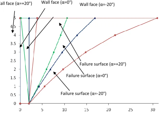
Fig. 10 shows the nonlinearity of failure surface of backfill (passive case) for different values of wall inclinations (α = -200
, 00, +200). It is seen that the failure angle increases with the increase in the wall inclination angles. For example, at Φ=30º, δ= Φ/2 and α = +20º, the value of failure angle at bottom is 64º whereas the value of failure angle at top is 55º. The comparison shows that the value of failure angle is 41.5º in case of Ghosh and Sengupta (2012) for the aforesaid conditions. Also Fig. 11 -12 shows that the failure wedge is quite different as compared to the failure surface of the Ghosh and Sengupta (2012) analysis. The surface shows curvilinear shape as it progresses upward.
Comparison of Failure Surface -
Fig.9 Shows the variations of passive earth pressure coefficient with respect to soil friction angle (Ф) for different surcharge loads (α = 200, δ= Ф/2).
Fig.10 Shows the nonlinearity of failure surface of backfill (passive case) for different values of wall inclinations, α = -200 , 00,+200 at Ф = 300, δ= Ф/2.
Wall face (α=+20°) Wall face (α=0°) Wall face (α=-20°)
Failure surface (α=-20°) Failure surface (α=0°)
4.4 Comparison of Results
Fig. 13 shows the variations of passive earth pressure coefficient with respect to soil friction angle (Φ) at Wall friction angles δ= Φ/2 for α = 200
. Kp increases uniformly with the increase in the value of soil friction angle (Φ). It can also
be observed from Table 2 that the value of Kp around 15% lesser than the values of Classical Coulomb (1776) theory.
Fig.11. Shows the comparison between failure surface of backfill (passive case) for wall inclination, α = +200 at Ф = 300, δ= Ф/2.
Fig.12 Shows the comparison between failure surface of backfill (passive case) for wall inclination, α = 00 at Ф = 300, δ= Ф/2.
Ø
Co-efficient of Passive earth pressure, Kp
δ α=-20 α=0 α=+20
10
0 1.745 1.420 1.358
Ø/2 2.023 1.568 1.444
Ø 2.351 1.727 1.543
20
0 2.933 2.039 1.754
Ø/2 4.331 2.625 2.061
Ø 7.044 3.481 2.493
30
0 5.204 3.00 2.216
Ø/2 12.096 4.909 3.146
Ø -- 9.643 4.732
40
0 10.246 4.599 2.898
Ø/2 -- 11.348 5.338
Ø -- -- 12.388
Table 2: Comparison of Results (Passive Case)
φ δ α Kp, Present study Kp, Coulomb (1776)
10 5 20 1.444 1.579
20 10 20 2.061 2.616
30 15 20 3.146 5.501
40 20 20 5.338 25.412
NOTATIONS
θ1 =Failure surface angle with vertical for top slice.
θn =Failure surface angle with vertical for bottom slice.
θR =Rate of change of failure surface angle.
Φ = Soil friction angle. δ = Wall friction angle.
α = Wall inclination angle with the vertical. Pp = passive earth pressure.
H1, H2 = horizontal shear.
ΔH = height of each slice. Wi = weight of i
th
slice. R = soil reaction force.
V1 = vertical load (UDL) acting on the bottom surface of the 1 st
layer. V2 = vertical load (UDL) acting on the top surface of the 1st layer.
γ = unit weight of soil.
V.
CONCLUSIONS
The present study provides an analytical model for the solution of passive earth pressure on the back of a battered face retaining wall supporting ϕ backfill. Using horizontal slice method, the solution of this model generates a non-linear failure surface and the value of passive earth pressure coefficients as obtained from this solution are of lesser magnitude in comparison to other available solutions like Coulomb (1776). The nature of the failure surface may be sagging or hogging in nature depending upon the soil-wall parameters. The results of the analysis are shown in tabular form and a detailed parametric study is done for the variation of different parameters. The present study shows that the seismic passive earth pressure co-efficient (Kp) increases due to the increase in wall friction angle (δ), soil friction angle (Φ) and surcharge (q); at
the same time the value of Kp decreases with the increase in wall inclinations (α).
REFERENCES
1. Coulomb, C.A. (1776), “Essai Sur Une Application Des Maximis et Minimis a Queques problems Des Statique Relatifsa1‟Architecture”, Nem. Div. Sav.Acad, Sci.Vol.7.
2. Rankine, W. J. M. (1857), “On the Stability of Loose Earth”, Phil. Tras. Royal Society (London). 3. Culmann, K. (1866), “Die Graphische Statik, Mayer and Zeller, Zurich.
4. Azad, A, Shahab Yasrobi, S. and Pak, A. (2008),“ Active Pressure Distribution History Behind Rigid Retaining Walls”, Soil Dynamics and Earthquake Engineering 28 (2008) 365-375
5. Ghanbari, A and Ahmadabadi, M. (2010), “Pseudo-Dynamic Active Earth Pressure Analysis of Inclined Retaining Walls Using Horizontal Slices Method” Transaction A: Civil Engineering Vol. 17, No. 2, pp. 118-130© Sharif University of Technology.